www.the-cryosphere.net/8/195/2014/ doi:10.5194/tc-8-195-2014
© Author(s) 2014. CC Attribution 3.0 License.
The Cryosphere
Effect of uncertainty in surface mass balance–elevation feedback on
projections of the future sea level contribution of the Greenland ice
sheet
T. L. Edwards1, X. Fettweis2, O. Gagliardini3,4, F. Gillet-Chaulet3, H. Goelzer5, J. M. Gregory6,7, M. Hoffman8,
P. Huybrechts5, A. J. Payne1, M. Perego9, S. Price8, A. Quiquet3, and C. Ritz3
1Department of Geographical Sciences, University of Bristol, Bristol BS8 1SS, UK
2Department of Geography, University of Liege, Laboratory of Climatology (Bat. B11), Allée du 6 Août, 2, 4000 Liège,
Belgium
3Laboratoire de Glaciologie et Géophysique de l’Environnement, UJF – Grenoble 1/CNRS, 54, rue Molière BP 96, 38402
Saint-Martin-d’Hères Cedex, France
4Institut Universitaire de France, Paris, France
5Earth System Sciences & Departement Geografie, Vrije Universiteit Brussel, Pleinlaan 2, 1050 Brussel, Belgium 6NCAS-Climate, Department of Meteorology, University of Reading, Reading, UK
7Met Office Hadley Centre, Exeter, UK
8Fluid Dynamics and Solid Mechanics Group, Los Alamos National Laboratory, T3 MS B216, Los Alamos, NM 87545, USA 9Department of Scientific Computing, Florida State University, 400 Dirac Science Library, Tallahassee, FL 32306, USA
Correspondence to: T. L. Edwards (tamsin.edwards@bristol.ac.uk)
Received: 8 February 2013 – Published in The Cryosphere Discuss.: 27 February 2013 Revised: 4 December 2013 – Accepted: 4 December 2013 – Published: 30 January 2014
Abstract. We apply a new parameterisation of the
Green-land ice sheet (GrIS) feedback between surface mass balance (SMB: the sum of surface accumulation and surface ablation) and surface elevation in the MAR regional climate model (Edwards et al., 2014) to projections of future climate change using five ice sheet models (ISMs). The MAR (Modèle At-mosphérique Régional: Fettweis, 2007) climate projections are for 2000–2199, forced by the ECHAM5 and HadCM3 global climate models (GCMs) under the SRES A1B emis-sions scenario.
The additional sea level contribution due to the SMB– elevation feedback averaged over five ISM projections for ECHAM5 and three for HadCM3 is 4.3 % (best estimate; 95 % credibility interval 1.8–6.9 %) at 2100, and 9.6 % (best estimate; 95 % credibility interval 3.6–16.0 %) at 2200. In all results the elevation feedback is significantly positive, am-plifying the GrIS sea level contribution relative to the MAR projections in which the ice sheet topography is fixed: the lower bounds of our 95 % credibility intervals (CIs) for sea
level contributions are larger than the “no feedback” case for all ISMs and GCMs.
Our method is novel in sea level projections because we propagate three types of modelling uncertainty – GCM and ISM structural uncertainties, and elevation feedback param-eterisation uncertainty – along the causal chain, from SRES scenario to sea level, within a coherent experimental design and statistical framework. The relative contributions to un-certainty depend on the timescale of interest. At 2100, the GCM uncertainty is largest, but by 2200 both the ISM and parameterisation uncertainties are larger. We also perform a perturbed parameter ensemble with one ISM to estimate the shape of the projected sea level probability distribution; our results indicate that the probability density is slightly skewed towards higher sea level contributions.
1 Introduction
The Greenland ice sheet (GrIS) response to climate change has two parts: surface mass balance (SMB), which is the sum of surface accumulation and surface ablation (broadly speaking, the balance of snowfall versus meltwater runoff); and dynamic, the changes in ice flow and discharge from the ice sheet. Various approaches to simulating these have been taken for making projections of the GrIS contribution to sea level. As with all simulation problems, there is a trade-off be-tween representing more processes, with the aim of increas-ing the physical realism of the simulations, and technical and computational resources, which limit implementation and the number of simulations.
The dynamic response is simulated with ice sheet models (ISMs), which solve the Stokes equations in complete or ap-proximate form. SMB can be simulated with sophisticated, physically based energy balance schemes in regional climate models (RCMs) such as MAR (Modèle Atmosphérique Ré-gional: Fettweis, 2007) and RACMO2/GR (e.g. Ettema et al., 2009). The two aspects of the GrIS response can thus be com-bined by forcing an ISM with SMB simulated by an RCM. But RCMs usually use a fixed surface topography, neglecting the important effects of ice sheet surface elevation changes on the atmosphere (Edwards et al., 2014) by omitting the SMB–elevation feedback. An alternative to using SMB from an RCM is to simulate it within the ISM, so that the evolv-ing ice sheet topography can dynamically alter the SMB. The most common approach to this is with a positive degree day (PDD) scheme, which parameterises SMB as a function of temperature and precipitation (supplied from observations for the present day, or a regional or global climate model for future projections) and possibly applies a simple snow-pack model (e.g. Janssens and Huybrechts, 2000). PDD mod-els incorporate the temperature aspect of the SMB–elevation feedback through a lapse rate correction, but not the precipi-tation aspect (except, in some cases, through a scaling factor for temperature), and also represent SMB much more simply than RCMs such as MAR and RACMO2/GR (Edwards et al., 2014).
To make the best use of physically based simulations of the GrIS response to climate change – simulating ice flow with an ISM and SMB with an RCM, while also including the SMB–elevation feedback – one can couple an ISM to an RCM. However, this is technically challenging and computa-tionally expensive, effectively precluding exploration of cli-mate and ice sheet modelling uncertainties.
The only way, therefore, to incorporate physical modelling of ice flow, SMB processes, and the SMB–elevation feedback while also exploring model uncertainties is with a parame-terisation such as the one we present in a companion paper (Edwards et al., 2014), where we characterise the SMB re-sponse to elevation in MAR using a suite of simulations in which the MAR GrIS surface height is altered. The param-eterisation is a set of four gradients, or “SMB lapse rates”,
that relate SMB changes to height changes below and above the equilibrium line altitude (ELA) and for regions north and south of 77◦N. Here we apply the parameterisation in five
ISMs to adjust MAR projections of SMB under the SRES A1B scenario (Naki´cenovi´c et al., 2000) as the ice sheet ge-ometry evolves.
The climate community have been attempting to quantify uncertainty in global climate model (GCM) predictions for some time, focusing on uncertainty in their parameter val-ues with perturbed parameter ensembles (PPEs) but also at-tempting to estimate structural uncertainty, which is uncer-tainty about the remaining discrepancy between a model and reality at the model’s most successful parameter values (e.g. Sexton et al., 2011; Sexton and Murphy, 2011). But proba-bilistic quantification of uncertainties in ice sheet model pre-dictions has hardly yet been attempted. There is also an ur-gent need to propagate uncertainties along the causal chain from greenhouse gas forcing scenarios to the impacts of cli-mate change. ISM projections are only beginning to tackle these challenges. Multi-model comparisons such as MIS-MIP (Pattyn et al., 2012) and SeaRISE (Bindschadler et al., 2013) compare ISMs with each other using standardised ex-periments, but the ice2sea project (http://www.ice2sea.eu) is among the first to explore systematically emissions scenarios and climate and ice sheet model uncertainties within a coher-ent framework (e.g. Rae et al., 2012; Fettweis et al., 2013).
In Edwards et al. (2014), we make uncertainty assessment an integral part of the parameterisation by estimating prob-ability distributions for the four parameters (elevation feed-back gradients). Here we propagate these uncertainties to fu-ture projections by sampling values from the four distribu-tions. We also use five different ISMs to assess the effect of ISM structural uncertainty that arises from different repre-sentations of ice flow and initialisation procedures, and ex-plore GCM structural uncertainty by forcing MAR with two different GCMs. Our coherent experimental design and sta-tistical framework, unusual in sea level projections, allow us to propagate the three types of model uncertainty along the causal chain from SRES scenario to sea level contribu-tion; assess the relative importance of these through time; and present probabilistic assessments of the effect of eleva-tion feedback parameterisaeleva-tion uncertainty on the projected GrIS sea level contribution under the A1B scenario.
2 Method
2.1 Climate projections
The regional climate model MAR (Fettweis, 2007) has been adapted for simulating the climate over Greenland, with full coupling to a complex snow/ice energy balance model and relatively high horizontal resolution (25 km). Unlike most RCMs, MAR includes the positive feedback between ice sur-face albedo and melting (Franco et al., 2013). We discuss the
processes and responses of MAR in more detail in Edwards et al. (2014).
We use five climate simulations performed for the ice2sea project. The first is a twenty year simulation of 1989–2008 in which MAR is forced at the boundaries by the ERA-INTERIM reanalysis (Dee et al., 2011), which we use as a baseline for initialisation and projections. The next two are twenty year simulations of 1980–1999 in which MAR is forced by two GCMs, ECHAM5 (Roeckner et al., 2003) and HadCM3 (Gordon et al., 2000), under 20th century cli-mate forcings, which we use to calculate projection anoma-lies. The final two are one hundred year projections (2000– 2099) forced by the two GCMs under the SRES A1B emis-sions scenario (Naki´cenovi´c et al., 2000). The A1B scenario is only defined until 2100, but we wish to make GrIS projec-tions for two hundred years (2000–2199). We did not have re-sources to simulate the second century (the climate respond-ing to the A1B scenario fixed at 2100 values), so we extend the MAR simulations by repeating the final decade (2090– 2099) ten times. This method is likely to underestimate the longer-term climate response, as discussed later.
MAR simulates SMB values only over grid cells cate-gorised as permanent ice, so the low spatial resolution (rel-ative to ISMs) leads to missing values for parts of the GrIS margin. As part of the data processing, we extrapolate the SMB field outwards from the ice sheet using a simpler repre-sentation of the SMB–elevation relationship than in Edwards et al. (2014). For each land grid cell, we use the ice grid cells within 100 km to fit a linear model of SMB versus surface height, and use this relationship with the land grid cell eleva-tion to assign an SMB value. This was performed before the parameterisation of Edwards et al. (2014) was developed.
2.2 Ice sheet models
We implement the parameterisation in five ISMs with vary-ing structure and complexity: Elmer/Ice, which solves the full Stokes equations; GISM, MPAS and CISM, which use a higher order approximation that reduces computational ex-pense (HO: e.g. Pattyn, 2003); and GRISLI, which uses a hy-brid of the first order shallow ice and shallow shelf approxi-mations (SIA and SSA: Bueler and Brown, 2009) to further reduce computational expense. We also use a SIA version of GISM, and call the two versions GISM-HO and GISM-SIA. Elmer/Ice and MPAS use finite element numerical methods on unstructured grids, while the others use finite difference methods on regular grids at 5 km resolution.
Elmer/Ice builds on Elmer, the open-source finite element, partial differential equation solving parallel code mainly de-veloped by the CSC-IT Center for Science Ltd in Finland. The unstructured mesh allows a variable grid resolution to focus computational resources at the ice sheet margin; here we use a minimum horizontal grid size of less than 1 km. GISM-SIA is a thermomechanical ISM (Huybrechts and de Wolde, 1999) that has been modified and extended for
pro-jections on centennial timescales using a new higher-order approximation of the force balance (GISM-HO: Fürst et al., 2011, 2013). The MPAS-Land Ice model is based on the MPAS (Model for Prediction Across Scales) climate mod-elling framework of Ringler et al. (2008); here we use a reg-ular 5 km resolution hexagonal mesh. GRISLI (GRenoble Ice Shelves and Land Ice model) is a thermomechanically cou-pled ISM; it is a hybrid model that for grounded ice uses the SIA for vertical shearing and the SSA as a sliding law (Ritz et al., 2001; Bueler and Brown, 2009). The Community Ice Sheet Model (CISM) version 2.0 includes improvements to all components of the Glimmer-CISM SIA model (Rutt et al., 2009). The models are summarised in Table 1; more detailed information is given elsewhere (Elmer/Ice: Gillet-Chaulet et al., 2012; GISM-HO: Goelzer et al., 2013; MPAS: Perego et al., 2012; CISM: Price et al., 2011; Lemieux et al., 2011; Evans et al., 2012; GRISLI: Quiquet et al., 2012).
2.3 Initialisation
Determining initial conditions for ISMs involves finding a balance between observations of the present-day ice sheet, reconstructions of past climate changes (to which the ice sheet is still responding), and the physical laws and parame-terised processes incorporated in the ISM, while accounting for uncertainties and limitations in all of these. ISM initiali-sation mostly uses ad hoc tuning methods rather than formal data assimilation as in numerical weather forecasting. Our initialisation procedures use observations of present-day ice sheet geometry (surface elevation, bedrock elevation and ice thickness; e.g. Bamber et al., 2013), ice velocities (Joughin et al., 2010; Bamber et al., 2000), and geothermal heat fluxes (Shapiro and Ritzwoller, 2004).
Methods vary between ISMs but in general there are three stages. First, we estimate the 3-D ice-temperature field by solving the heat equation, in some cases accounting for the response to atmospheric temperature changes over one or more glacial–interglacial cycles. Second, we infer the spa-tial pattern of the basal drag coefficient that leads to the best agreement with observed ice velocities, given observational uncertainties and model limitations. During these first two stages, the geometry of the ice sheet is held constant to the observed values (Bamber et al., 2013). For the third stage, we finally allow the ice sheet geometry to evolve or “relax” so that it is internally consistent with the ice temperature and flow fields.
We derive ice temperatures for Elmer/Ice using the com-putationally cheaper SIA model SICOPOLIS (Greve, 1997). We derive them for CISM, MPAS and GRISLI from a quasi-steady-state CISM simulation forced with a constant sur-face temperature field simulated by the RACMO/GR re-gional climate model (Ettema et al., 2009, as specified in the SeaRISE project protocol: http://websrv.cs.umt.edu/isis/ index.php/Present_Day_Greenland). We obtain ice tempera-tures for the two GISM models from a GISM-SIA simulation
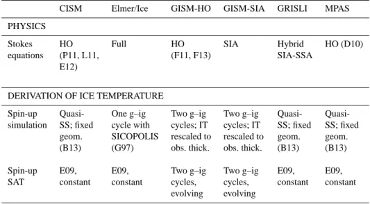
Table 1. Summary of ice sheet model (top) treatment of Stokes equations and (bottom) derivation of ice temperature (IT) boundary conditions. HO, SIA and SSA are higher order, shallow ice and shallow shelf approximations; SS is steady state; SAT is surface air temperature data used for the spin-up simulation; g–ig is glacial–interglacial. All models use bedrock elevation data from Bamber et al. (2013) and geothermal heat flux from Shapiro and Ritzwoller (2004). References: B13: Bamber et al. (2013); D10: Dukowicz et al. (2010); E09: Ettema et al. (2009); E12: Evans et al. (2012); F11, F13: Fürst et al. (2011) and Fürst et al. (2013); G97: Greve (1997); L11: Lemieux et al. (2011); P11: Price et al. (2011).
CISM Elmer/Ice GISM-HO GISM-SIA GRISLI MPAS
PHYSICS
Stokes HO Full HO SIA Hybrid HO (D10)
equations (P11, L11, (F11, F13) SIA-SSA
E12)
DERIVATION OF ICE TEMPERATURE
Spin-up Quasi- One g–ig Two g–ig Two g–ig Quasi-
Quasi-simulation SS; fixed cycle with cycles; IT cycles; IT SS; fixed SS; fixed
geom. SICOPOLIS rescaled to rescaled to geom. geom.
(B13) (G97) obs. thick. obs. thick. (B13) (B13)
Spin-up E09, E09, Two g–ig Two g–ig E09, E09,
SAT constant constant cycles, cycles, constant constant
evolving evolving
of several glacial–interglacial cycles, rescaling the ice tem-perature field to the observed ice thickness (Goelzer et al., 2013). Geothermal heat flux fields in all spin-up simula-tions are from Shapiro and Ritzwoller (2004). Ice tempera-ture spin-up simulations are summarised in Table 1.
We infer the basal drag coefficient from observed ve-locities using the control method (Elmer/Ice: Morlighem et al., 2010), an iterative inverse method (GRISLI), or tun-ing (CISM, MPAS); the methods and velocity targets are also summarised in Table 1.
We obtain the initial ice sheet geometry by forcing the ISM with a present-day mean SMB field. For most mod-els this is the 1989–2008 mean (the reference period for the ice2sea project) of the ERA-INTERIM forced MAR simu-lation; for GISM we use the 1960–1990 mean SMB calcu-lated with the GISM PDD scheme from ERA-40 data (Up-pala et al., 2005) and observed surface elevation (similar to Hanna et al., 2011). We obtain the initial geometry for Elmer/Ice by allowing the upper surface to evolve for 55 yr under the present-day SMB forcing, and use the same ini-tial geometry for GRISLI, allowing it to evolve for a fur-ther 145 yr to obtain a coherent initial state for this model. We initialise the GISM models by allowing the geometry to evolve for 1000 yr while the ice sheet margin is fixed to observed values under present-day SMB forcing and ice thickness changes are limited to 0.2 m a−1. These relaxation periods are determined arbitrarily or by available computa-tional resource, though most of the flux divergence anomalies that arise from observational and modelling uncertainties die away after a few years (e.g. Gillet-Chaulet et al., 2012). We
do not relax the geometry for CISM and MPAS. However, these simulations are already closer to the present-day state than for the other models because they use a quasi-steady-state spin-up forced with modern-day surface temperatures, rather than glacial–interglacial cycles, and calibrate the basal drag with balance velocities (which have complete coverage and are in equilibrium with the geometry), rather than surface velocities.
We use two methods to correct any remaining drift that arises from model imbalances. For Elmer/Ice and GRISLI, we perform a control simulation and subtract this from the results (Sect. 2.5). For the others we diagnose and apply a “synthetic SMB” correction, which is the additional SMB required to keep the ice sheet close to the present-day ob-served geometry under present-day SMB forcing. The syn-thetic SMB correction is applied unaltered in perturbed simu-lations (i.e. the parameterisation adjusts only the MAR SMB forcing and not the synthetic SMB correction). This is sim-ilar, in principle, to the flux corrections that were formerly in common use in atmosphere–ocean GCMs. In CISM and MPAS there is no relaxation in the initialisation procedure, so the synthetic SMB accounts for the entire initial mass imbal-ance generated by the initial geometry. The mean synthetic SMB correction for both GISM models is 9 cm a−1, with less
than 0.3 % of the total ice sheet area having a correction of greater than 10 m a−1, mainly at marine-terminating ice mar-gins (Goelzer et al., 2013). For MPAS the mean synthetic SMB correction is −7.3 cm a−1, with 1.6 % of the total ice sheet area having a correction of greater than 10 m a−1, and
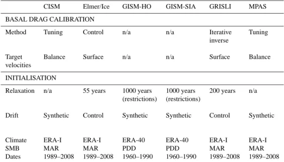
Table 2. Summary of ice sheet model basal drag calibration and initialisation. PDD is positive degree day.
CISM Elmer/Ice GISM-HO GISM-SIA GRISLI MPAS
BASAL DRAG CALIBRATION
Method Tuning Control n/a n/a Iterative Tuning
inverse
Target Balance Surface n/a n/a Surface Balance
velocities
INITIALISATION
Relaxation n/a 55 years 1000 years 1000 years 200 years n/a
(restrictions) (restrictions)
Drift Synthetic Control Synthetic Synthetic Control Synthetic
Climate ERA-I ERA-I ERA-40 ERA-40 ERA-I ERA-I
SMB MAR MAR PDD PDD MAR MAR
Dates 1989–2008 1989–2008 1960–1990 1960–1990 1989–2008 1989–2008
for CISM it is 2.4 cm a−1, with less than 2 % of the total ice sheet area having a correction of greater than 10 m a−1.
We exclude Greenland’s glaciers and ice caps from the projection results using a mask produced for ice2sea (Rastner et al., 2012).
The basal drag calibration and initialisation methods are summarised in Table 2. More details can be found in the ref-erences given in the previous section and the table.
2.4 Boundary conditions
The boundary conditions are geothermal heat flux, ice temperature, bedrock elevation, and projections of SMB. Geothermal heat fluxes are from Shapiro and Ritzwoller (2004) and held fixed in the simulations. We also keep the ice temperature fields (determined during initialisation; Sect. 2.3 and Table 1) held fixed because there is negligible ice tem-perature response to changing atmospheric forcing over two centuries. We use bedrock elevations from the ice2sea data set (Bamber et al., 2013) and hold these fixed because there is negligible isostatic adjustment on this timescale (e.g. Goelzer et al., 2013).
The SMB forcings are therefore the only time-varying boundary conditions. We force the ISMs with “anomaly-corrected” SMB projections, SRCM0, to remove the mean discrepancy in MAR between the GCM-forced and ERA-INTERIM reanalysis-forced simulations (Fettweis et al., 2013). For this we calculate SMB anomalies with respect to the present day by subtracting the 1989–2008 mean SMB (1989–1999: 20th century climate forcings; 2000– 2008: A1B scenario) from the A1B projections. We add these anomalies to the present-day SMB used for initialisation, to
give
S2000,...,2199RCM0 =S2000,...,2199A1B −S1989−200820C,A1B +Sinit,
where Sinit is generally S1989−2008ERAI , the 1989–2008 mean of the ERA-INTERIM forced simulation (except GISM, SERA401960−1990). If used, the synthetic SMB field is also applied. Our initialisation and anomaly-correction methods use the approximation that SMB trends during the period 1989–2008 are small relative to the A1B projections (Rae et al., 2012).
2.5 Parameterisation
We use the SMB–elevation feedback parameterisation to ad-just the anomaly-corrected SMB forcing as the GrIS surface height in each ISM evolves. The adjustment is made each year, for each grid cell, using one of four parameters (gradi-ents) selected according to the current “reference” SMB and the region of the grid cell (Edwards et al., 2014).
For a given ISM grid cell in a given year (t), a gradient (bt)
(kg m−3a−1) is used to adjust the SMB forcing (kg m−2a−1) using the height difference (m) between the previous year and the start of the simulation:
Stadj=StRCM0+bt(hISMt −1−h ISM 0 ),
where Stadj is the adjusted SMB, StRCM0 is the anomaly-corrected RCM SMB, and hISMt is the ISM height. The gra-dient bt is selected from one of four values according to the
reference SMB (Sref<0 or Sref≥0) and region (north or south of 77◦N) of the grid cell, where Strefis the mean Sadj of the previous decade or, for the first decade, all available years.
In Edwards et al. (2014), we estimate probability distri-butions for each of the four parameters (gradients). Our best estimate values of the parameters are the modes of these four distributions, and our credibility intervals (CIs) encompass the central 95 % of each. We propagate the parameter un-certainties to sea level projections by performing simulations using different values sampled from the distributions: (a) the four modes, i.e. best estimates; (b) the four 2.5 % quantiles, i.e. lower bounds of the CIs; and (c) the four 97.5 % quan-tiles, i.e. upper bounds. The parameter estimates are given in Table 3. They differ slightly to those in Edwards et al. (2014) due to changes made to the parameter estimation code for an update to that study: a small error was corrected, unnecessary rounding was removed, and the code was restructured (thus changing the random seed for bootstrapping). One difference is 0.03 (SMB ≥ 0, 97.5 % bound), and the other differences are 0.02 or less.
With one model, GISM-SIA, we also sample the four dis-tributions more thoroughly by using 99 percentiles: i.e. the four 1 % quantiles in one simulation; the four 2 % quantiles in the next, and so on up to the four 99 % quantiles.
We therefore generate five simulations for each ISM:
– Control: forced with Sinit (Elmer/Ice, GRISLI) or
Sinit+Ssyn (other models), to check for or subtract model drift from the projections;
– No feedback: forced with SRCM0 with no adjustment,
to estimate the response of the GrIS without elevation feedback;
– Best estimate: forced with Sadj, using the “best
esti-mate” values of the four parameters (Table 3);
– 2.5 % and 97.5 % quantiles: as for best estimate, but
using the parameter values that correspond to the bounds of the 95 % CI (Table 3).
We perform these for the two MAR simulations forced by ECHAM5 (all ISMs) and HadCM3 (Elmer/Ice, GISM-HO, GISM-SIA and GRISLI) under the A1B scenario over 2000– 2200. As described above we also use GISM-SIA to perform a simulation with each of the 99 percentile estimates of the four parameters, forming a 99 member PPE; we do this only for the ECHAM5 projection.
The drift in the control simulations is very small (0.03 %, or less, of the cumulative projected sea level contribution at 2200) for all models except Elmer/Ice, which has a drift of 2– 2.5 % (−4 mm). For this model, drift is not constrained dur-ing the initialisation procedure and the free-surface elevation has been allowed to diverge from observations for a relax-ation period of only 55 yr. The applied SMB is not corrected by a synthetic SMB, and the remaining drift shows the drift of the model when directly applying the 1989–2008 mean SMB given by MAR forced under ERA-INTERIM. This drift is corrected by subtracting the control simulation from the projections.
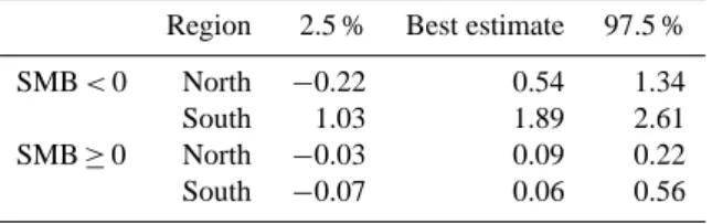
Table 3. The 2.5 % quantile, best estimate, and 97.5 % quantile
estimates of the SMB–elevation gradients in kg m−3a−1, below
(SMB < 0) and above (SMB ≥ 0) the ELA, for regions north and
south of 77◦N.
Region 2.5 % Best estimate 97.5 %
SMB < 0 North −0.22 0.54 1.34
South 1.03 1.89 2.61
SMB ≥ 0 North −0.03 0.09 0.22
South −0.07 0.06 0.56
3 Results
The additional cumulative sea level contribution due to the SMB–elevation feedback, under the A1B scenario and aver-aged over five ISM projections for ECHAM5 and three for HadCM3, is 4.3 % (best estimate; 95 % credibility interval 1.8–6.9 %) at 2100, and 9.6 % (best estimate; 95 % credibil-ity interval 3.6–16.0 %) at 2200 (Figs. 1 and 2; Tables 4 and 5). We exclude GISM-SIA from summary statistics because it is so similar in structure, and identical in set-up, to GISM-HO that it would effectively give double weighting to GISM. In all ISM predictions the elevation feedback is positive: the lower bounds of the 95 % CIs (the 2.5 % quantile simu-lations) are always larger than the “no feedback” case. This amplifying effect is expected, because mean GrIS SMB be-comes negative at around 2050 (Rae et al., 2012) and the gradient estimates for negative SMB are generally positive (Edwards et al., 2014) thus adjusting the SMB in the same direction: more negative, giving greater sea level contribu-tion. However, this was not guaranteed, because there are both positive and negative values in the mean SMB forcing, in the SMB changes from 2000–2199, and in the gradient sets (Edwards et al., 2014).
The larger feedback adjustment at 2200 arises from the negative SMB forcing at the end of the first century which is sustained (by repetition of the decade 2090–2099 from the MAR simulation: Sect. 2.1) during the second century.
The Elmer/Ice and GRISLI total sea level contributions are virtually identical, but this is a coincidence: the changes in ice discharge and SMB are different, and the differences just compensate each other so that the sea level contributions are the same. The two models do have similar initialisation procedures, but the differing dynamic and SMB responses lead us to believe this is not the reason for the similar results. CISM seems to be an outlier in the ISM ensemble, particu-larly at 2200 (Fig. 2; Table 5), in both the no feedback result (low) and the magnitude of the feedback (small), though the latter may be a result of the former. The GISM-SIA results are very similar to those of GISM-HO. This can be explained by the identical model set-up and their similarity in response to perturbations; the only difference between the two models is in the dynamic response, which is a much smaller contri-bution than the SMB response (Fürst et al., 2013).
Table 4. Projected sea level contribution (mm) at 2100 for the ECHAM5 (top) and HadCM3 (bottom) A1B projections: no feed-back, 2.5 % quantile, best, and 97.5 % quantile estimates.
Model No 2.5 % Best 97.5 % feedback estimate ECHAM5 CISM 53.7 53.8 54.7 56.9 Elmer/Ice* 57.0 58.2 59.8 60.9 GISM-HO* 55.7 56.8 58.3 59.8 GISM-SIA 56.6 57.6 59.2 60.6 GRISLI* 57.1 58.1 59.6 61.0 MPAS 57.4 58.4 60.0 61.4 Mean (*) 56.6 57.7 59.2 60.5 HadCM3 Elmer/Ice* 64.8 66.1 67.9 69.2 GISM-HO* 62.9 64.3 66.0 67.7 GISM-SIA 63.5 64.9 66.7 68.3 GRISLI * 64.7 66.0 67.7 69.3 Mean (*) 64.1 65.4 67.2 68.7
We can compare ECHAM5 and HadCM3 using the three ISMs that used both projections (Elmer/Ice, GISM-HO and GRISLI, from here on called the “starred” models). The HadCM3-forced projection gives consistently higher sea level contributions than the ECHAM5-forced, because the HadCM3-forced MAR simulation projects greater meltwa-ter runoff (Rae et al., 2012). Without elevation feedback, the mean GrIS sea level contributions at 2100 are 57 mm for ECHAM5 and 64 mm for HadCM3; with feedback, these increase by 3 mm (5 %). At 2200, the mean contributions without feedback are 164 mm for ECHAM5 and 176 mm for HadCM3; the feedback contributes an additional 16 mm (10 %) and 19 mm (11 %), respectively.
Not only does the contribution due to the feedback in-crease with time, but so does the uncertainty. Our experi-mental design allows us to inspect the changes and relative importance of the different modelling uncertainties. At 2100 (Fig. 1; Table 4), the GCM differences are, respectively, 2.6 and 1.7 times those of the elevation feedback parameterisa-tion and ISM uncertainties: the mean difference between the two GCMs (averaged over the no feedback and three feed-back estimates) for the three starred models is 7.8 mm; the mean spread of all five ISMs for ECHAM5 is 4.5 mm; and the mean 95 % CI (over all ISMs and GCMs) is 3.0 mm. But by 2200 (Fig. 2; Table 5), the relative importance has changed. The ISM spread and elevation feedback param-eterisation uncertainty overtake the difference between the two GCMs: the mean difference between the two GCMs is 13.7 mm; the mean spread of ISMs for ECHAM5 is 25.8 mm; and the mean 95 % CI (over all ISMs and GCMs) is 20.8 mm.
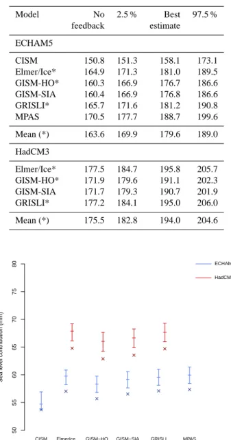
Table 5. As for Table 4, but at 2200.
Model No 2.5 % Best 97.5 % feedback estimate ECHAM5 CISM 150.8 151.3 158.1 173.1 Elmer/Ice* 164.9 171.3 181.0 189.5 GISM-HO* 160.3 166.9 176.7 186.6 GISM-SIA 160.4 166.9 176.8 186.6 GRISLI* 165.7 171.6 181.2 190.8 MPAS 170.5 177.7 188.7 199.6 Mean (*) 163.6 169.9 179.6 189.0 HadCM3 Elmer/Ice* 177.5 184.7 195.8 205.7 GISM-HO* 171.9 179.6 191.1 202.3 GISM-SIA 171.7 179.3 190.7 201.9 GRISLI* 177.2 184.1 195.0 206.0 Mean (*) 175.5 182.8 194.0 204.6 Sea le v el contr ib ution (mm) 50 55 60 65 70 75 80
CISM ElmerIce GISM−HO GISM−SIA GRISLI MPAS
ECHAM5
HadCM3
Fig. 1. Projected cumulative GrIS sea level contributions for the ECHAM5 and HadCM3 A 1B projections at 2100. Crosses mark simulations with no elevation feedback. Bars mark the estimated 95 % credibility intervals and (central tick) best estimates of the el-evation feedback parameterisation.
In other words, the parameterisation and ISM uncertainties increase by a factor of seven and six, respectively, between 2100 and 2200, while the difference between the two GCMs barely doubles. The relative contributions to our uncertainty thus depend on the timescale of interest.
This can be seen clearly in Fig. 3, which shows the frac-tional uncertainties as a function of time with a 15 yr run-ning mean applied. Although we have a small number of ice sheet and climate models, it is useful to examine the relative importance of different uncertainties in our study to inform
Sea le v el contr ib ution (mm) 140 150 160 170 180 190 200 210 220
CISM ElmerIce GISM−HO GISM−SIA GRISLI MPAS
ECHAM5 HadCM3
Fig. 2. As for Fig. 1, but at 2200.
2000 2050 2100 2150 2200 0.0 0.2 0.4 0.6 0.8 1.0 Year Fr actional uncer tainty Parametric (95% CL) GCM (range) ISM (range)
Fig. 3. Fractional uncertainties in projected cumulative GrIS sea level contributions for elevation feedback parameterisation (95 % credibility interval divided by best estimate, averaged over ISMs and GCMs; GCMs (difference between ECHAM5 and HadCM3 di-vided by their mean, averaged over ISM best estimates; and ISMs (range of ISM best estimates divided by their mean, for ECHAM5 projections). A 15 yr running mean is applied.
future work: for example, determining which uncertainties are largest in our experimental design, and how others may therefore choose to prioritise their computational resources. At the start of the projections, the ISM structural uncertainty explored (the range of five ISM best estimates divided by their mean, for the ECHAM5 projections) is a large frac-tion because the signal is small, but the fracfrac-tion decreases (the signal increases faster than the range) during the first half of the twentieth century. After this the fraction increases
Sea level contribution (mm)
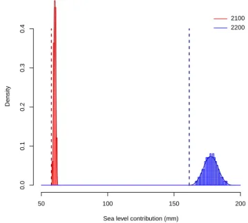
Density 50 100 150 200 0.0 0.1 0.2 0.3 0.4 2100 2200
Fig. 4. GISM-SIA projections for sea level contribution in 2100 (red) and 2200 (blue): no elevation feedback (dashed vertical line) and with feedback (histograms and density estimates).
again (the range increases faster than the signal). The time dependence of the GCM structural uncertainty explored (the difference between ECHAM5 and HadCM3 results divided by their mean, averaged over the best estimates for the three starred ISMs) appears at first glance to be similar, but the underlying reason is different: it rapidly falls to a mini-mum when the two GCMs projections happen to coincide for a short period (see also Rae et al., 2012). After a short increase due to the GCMs diverging again, the fractional un-certainty slowly falls because the signal increases faster than the range. The fractional uncertainty due to the parameterisa-tion (95 % CI divided by the best estimate, averaged over all ISMs and GCMs) is initially very small, but increases fairly linearly with time: the width of the CI scales with the sig-nal. In the latter part of the second century the parameteri-sation uncertainty overtakes that of the GCMs. These results are discussed further in the next section.
The 99 member GISM-SIA PPE gives the entire sea level probability distribution (Fig. 4) because it jointly samples the full probability distributions of each of the four gradient parameters rather than just the bounds of the 95 % CIs. We can inspect any other interval, such as the 90 % CI (177.3– 194.7 mm) or 50 % CI (182.3–190.6 mm). We can also test whether the projected distribution of sea level contributions is symmetric about the best estimate of 186.1 mm. The 95 % CI is symmetric (±10.4 mm), and the 90 % CI nearly so (−8.8 mm, +8.6 mm), but the 50 % interval (−3.8 mm,
+3.5 mm) indicates the probability density leans slightly to-wards the higher sea level contributions.
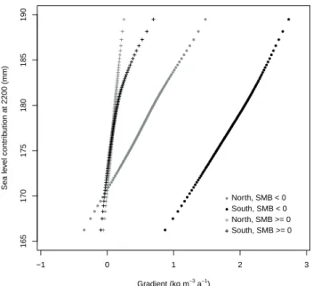
−1 0 1 2 3 165 170 175 180 185 190 Gradient (kg m−3 a−1 ) Sea le v el contr ib ution at 2200 (mm) ● ● ● ● ● ● ● ●● ●● ●● ●● ●●● ●●●●●●●●●●●●●●●●●●●●●●●●●●●●●●●●●●●●●●●●●●●●●●●●●●●●●●●●●●●●●●●●●●● ●●● ●● ●● ● ● ● ● ● ● ● ●North, SMB < 0 ● ● ● ● ● ● ● ●● ●● ●● ●● ●●● ●●●●● ●●●●●●●●●●●●●●●●●●●●●●●●●●●●●●●●●●●●●●●●●●●●●●●●●●●●●●●●●●●●●● ●●● ●● ●● ● ● ● ● ● ● ● ●South, SMB < 0 North, SMB >= 0 South, SMB >= 0
Fig. 5. GISM-SIA projections for sea level contribution in 2200 as a function of elevation feedback gradient values.
The unimodal and (broadly) symmetric shape of the PPE sea level distribution is probably a result of the unimodal and (in most cases) symmetric shapes of the four posterior prob-ability distributions of the gradient values (Edwards et al., 2014), combined with the linear model of adjustment. Fig-ure 5 shows the dependence of the sea level contribution on the gradient sets. However, this cannot show which of the four gradients is most important because they are varied jointly. But it illustrates some characteristics of the param-eterisation structure and uncertainties: first, the relationship between sea level contribution and SMB lapse rates is fairly linear, save for a clear change in slope for the south SMB ≥ 0 lapse rate. This is due to the linear adjustment model, but is perhaps surprisingly robust considering the SMB ≥ 0 lapse rates range from negative to positive values, and considering there is a positive feedback in adjusting SMB. In fact the lat-ter effect can be seen in the SMB < 0 slopes, which become slightly steeper at larger SMB lapse rates. Second, the mag-nitude of the slopes illustrate the characteristics of the SMB lapse rate probability distributions (Edwards et al., 2014): shallower slopes for the two SMB < 0 lapse rates are a result of their broader probability distributions, i.e. larger absolute uncertainties, relative to the SMB ≥ 0 lapse rates. Similarly, the south SMB ≥ 0 slope change is due to the asymmetric probability distribution.
4 Discussion
4.1 Elevation feedback
It is important to quantify the SMB–elevation feedback, rela-tive to projections without it (such as Rae et al., 2012), to im-prove our assessments of GrIS sensitivity to climate change. Using RCMs to simulate SMB represents the processes more fully than with ISMs; using ISMs to evaluate the feedback it-self gives a more complete picture than with RCMs alone (by modifying their topography), because they simulate the en-tire GrIS response rather than only the SMB aspect. Param-eterising the SMB–elevation feedback gives the best of both worlds, allowing ISMs to be forced with SMB from RCMs and include the feedback, while being computationally cheap enough to explore model uncertainties. The response of SMB to changes in ice surface elevation is complex and nonlinear, and even with a probabilistic uncertainty assessment, a lin-ear parameterisation cannot fully represent the SMB changes that would be modelled by a fully coupled RCM-ISM. How-ever, the advantages of our particular parameterisation over other studies are described in the companion paper (Edwards et al., 2014).
We present the first application of an SMB–elevation pa-rameterisation to RCM projections of future sea level rise. The feedback always increases sea level rise, even for the lower bounds of our 95 % CIs (despite the negative gradient values: Table 3). But the additional contribution is relatively small, with best estimates 4.3 % at 2100 and 9.6 % at 2200.
We can compare these results with estimates from the RCM alone. When MAR is forced by the GCM MIROC5 under the Representative Concentration Pathway RCP8.5 (Moss et al., 2010), changing the ice sheet height by an amount equivalent to cumulative projected SMB changes from 2000–2079 gives a much greater feedback contribution than our result: 5–15 % over just one century (Fettweis et al., 2013). At first glance this might appear to be due to the use of a high-end scenario (relative to the medium scenario A1B), giving larger SMB changes and therefore a larger feedback.
However, the greater feedback contribution in the RCM most likely arises from the absence of ice dynamics. Perhaps counter-intuitively, sea level rise from the total GrIS response (SMB and dynamics) is smaller than from the SMB response alone. Recent ice2sea studies (e.g. Gillet-Chaulet et al., 2012; Goelzer et al., 2013) have highlighted the complexity of the interactions between SMB and dynamic responses. Dynamic mass loss and SMB-related mass loss are not additive: mass loss by one process decreases loss by the other, so we cannot neatly divide sea level contributions into, for example, 60 % SMB and 40 % dynamic. SMB removes ice (e.g. through melting) before it can reach the ice sheet margin to be dis-charged. Conversely, dynamics remove ice before it can melt and also partly compensate surface height decreases (from increased melting) by redistributing mass gained at the top of the ice sheet, thickening the ablation zone and therefore
reducing melting. Further discussion can be found in Gillet-Chaulet et al. (2012) and Goelzer et al. (2013), though this is not a recent finding: Huybrechts and de Wolde (1999), for example, find a 24 % lower sea level contribution by 2100 from Greenland when dynamics are included. In our study the time integrated SMB changes for the ECHAM5-forced MAR simulation contribute 62.7 mm to sea level by 2100 and 211.4 mm by 2200 (Goelzer et al., 2013), while the total responses from the ice sheet models are substantially smaller: 53.7–57.4 mm at 2100 and 150.8–170.5 mm at 2200 (Tables 4 and 5).
Therefore, it is not surprising that SMB-only projections, without coupling to an ice sheet model, show larger SMB– elevation feedback contributions. The results from Fettweis et al. (2013) are likely overestimates. Only a coupled RCM-ISM would allow full evaluation of this response, but our results suggest that the feedback effect is small enough that using such models for one- or two-century simulations may not be justified given the additional computational expense, technical difficulty, and severe restrictions on exploring mod-elling uncertainties.
We can also compare these results with estimates from an ISM alone. Some have previously suggested that the sim-pler PDD descriptions of ice sheet response are too sen-sitive to climate change (van de Wal, 1996; van de Berg, 2011), but recent studies find they are less sensitive than MAR and RACMO/GR (Goelzer et al., 2013; Helsen et al., 2011; Vernon et al., 2013; Hanna et al., 2011). Goelzer et al. (2013) compare projections from our parameterisation ver-sus the GISM PDD scheme, using the same ice sheet extent and RCM, and Helsen et al. (2011) compare their param-eterisation of the RACMO2/GR SMB–elevation feedback with PDD results. In both cases the PDD schemes predict a smaller sea level contribution in a warmer climate than the RCMs: for example, Goelzer et al. (2013) find the PDD model gives a 31 % lower sea level contribution than MAR. There are many differences between physically based energy balance RCM schemes and empirical PDD schemes, includ-ing the presence of albedo feedback in the RCMs, higher spatial resolution in the PDD schemes, and different treat-ment of refreezing (Goelzer et al., 2013). Our parameterisa-tion of the SMB–elevaparameterisa-tion feedback is more complex than a PDD scheme, in that it estimates probability distributions rather than a fixed lapse rate, includes nonlinear precipita-tion aspects, and incorporates variaprecipita-tion of the feedback with climate, topography and region (through the use of four prob-ability distributions).
This parameterisation could be used to correct low resolu-tion MAR simularesolu-tions onto a high resoluresolu-tion digital elevaresolu-tion map; the difference in elevation between the two topogra-phies is analogous to the geometry evolution in ISM simu-lations. This correction might improve the realism of MAR SMB simulations, which would be useful not only for forcing ISMs but also comparing with observations.
4.2 Modelling uncertainties
It is a research priority to improve quantification of ice sheet model uncertainties, so as to make meaningful and complete statements about the difference between our projections and the real world. Research in this area is sparse, but the ice sheet modelling community can make rapid improvements by applying established uncertainty quantification techniques from climate and other environmental modelling research ar-eas, as we have done here.
Our method is novel because we propagate three types of model uncertainty – GCM structural uncertainty, ISM struc-tural uncertainty, and elevation feedback parameterisation uncertainty – along the causal chain from SRES scenario to sea level within a coherent experimental design and statis-tical framework. In particular, parameter uncertainty is esti-mated with a probabilistic method, which gives well-defined credibility intervals (CIs) rather than simple sensitivity anal-ysis; all ISMs use the same parameterisation and parameter sampling, and are forced with the same GCMs and RCM, enabling comparisons across ISMs; and MAR is forced with two GCM forcings under the same SRES scenario, enabling comparisons between ECHAM5 and HadCM3. A similar ap-proach is taken by Shannon et al. (2013) for a new parame-terisation of GrIS basal lubrication. This experimental de-sign gives us the opportunity to assess the relative importance of various modelling uncertainties and how these vary with time. We discuss parametric uncertainties, structural uncer-tainties, time dependence, and future directions.
The feedback parameter uncertainties translate to a uni-modal and fairly symmetric probability distribution for sea level contribution (Fig. 4), because of the linear SMB adjust-ment and the sampling from unimodal and (in most cases) symmetric probability distributions for the gradients (Ed-wards et al., 2014). If the gradient distributions derived from MAR were strongly asymmetric or multimodal, or the SMB adjustment nonlinear, the sea level distribution might be a different shape. Here is the real value of Bayesian param-eter estimation (Edwards et al., 2014) and sampling these uncertainties with perturbed parameter ensembles, because such things are generally not known in advance. The slight asymmetry in the sea level probability distribution described in the previous section might become more pronounced for timescales longer than two centuries.
If substantially greater computational and time resources were available, a natural next step might be a more thor-ough exploration of parametric uncertainties, by simultane-ously perturbing additional parameters of the ISMs and, if possible, parameters of the climate models. Climate model PPEs are used extensively (e.g. Murphy et al., 2009); RCM PPEs are relatively rare due to their computational expense (e.g. Sexton and Murphy, 2011). Two ISM PPEs are pre-sented by Stone et al. (2010) and Applegate et al. (2011), who vary multiple parameters simultaneously in order to explore their interactions. For example, surface lowering driven by
parameterised dynamic processes (such as basal lubrication: Shannon et al., 2013) could interact differently with the ele-vation feedback depending on the values of the relevant pa-rameters. Performing multiple parameter perturbations might affect the shape of the distribution of projected sea level con-tributions.
Structural uncertainties are much more challenging to quantify. Using multi-model ensembles is a necessary first step. But there is no well-defined space from which to sample (as there is for parameters). Models have common compo-nents and errors that are likely to reduce the ensemble range relative to our uncertainty about the climate and GrIS. It is extremely difficult to express this probabilistically – to quan-tify the degree to which the spread of a model ensemble en-compasses our true uncertainty about the system – and there is no consensus about how to do so. Given these difficulties, and our small ensemble sizes, we do not claim to quantify ISM and GCM structural uncertainties, only to sample from them. It is better to sample from this space, to explore it par-tially, than to ignore it. Coherent experimental design such as this – systematic sampling of models, parameterisation, and parameter values – is essential to better understanding of structural uncertainties.
The structural uncertainty we explore most is in the ISMs. This arises from structural differences in ice sheet modelling, including representation of the Stokes equations, numerical methods, grid resolution, initialisation procedures, and drift correction. Given these differences, it might seem surprising that the results from different ice sheet models are so similar. Goelzer et al. (2013) compare GrIS sea level projections with different plausible modelling choices for a single ice sheet model (GISM-HO) and the same RCM (MAR) and GCM (ECHAM5) as here, and obtain a wider range of projections. But our results confirm the importance of SMB versus dy-namic mass loss. The large spread in results in Goelzer et al. (2013) arises from differing SMB projections: an RCM, a PDD model forced with an RCM, and a PDD model forced with a GCM. In our study all models (by definition) use the same projected SMB changes, and also use the same mask to define ice sheet extent (Sect. 2.3). The dynamical response of the GrIS is smaller than the SMB response, so differ-ences in model physics, numerical methods, grid and even initialisation cannot substantially alter the sea level contribu-tion: SMB is the dominant driver of sea level rise. This con-firms results by others such as Gillet-Chaulet et al. (2012) and Goelzer et al. (2013).
We use only two GCMs and do not explore RCM struc-tural uncertainty at all. We do incorporate uncertainty in the structure of our parameterisation of MAR, by including a dis-crepancy variance term when estimating the gradients (Ed-wards et al., 2014), but this refers to our parameterisation of the MAR elevation feedback, not the MAR simulation of the feedback in the real world; the latter is the RCM structural uncertainty. We could sample RCM structural uncertainty us-ing multiple RCMs, but this is extremely challengus-ing due to
their computational expense. An ensemble of RCMs would also require a new parameterisation of the SMB–elevation feedback for each. For further exploration of MAR and GCM uncertainties, we refer to Fettweis et al. (2013) who evalu-ate the effects of changing the MAR tundra/ice mask and ice sheet topography, and using a range of GCMs for forcing, on simulations of current climate and projections of future climate change.
We therefore do not claim to make a full assessment of modelling uncertainty in sea level projections. Such an as-sessment would require perturbing other parameters of the ice sheet models, perturbing parameters of the climate mod-els, and quantifying ice sheet model and climate model structural uncertainties through, for example, large multi-model ensembles of ISMs, RCMs and GCMs. This is be-yond present capabilities, though we believe it should be our aim. These additional uncertainties have potentially large ef-fects on predictions of future mass loss, which would result in wider credibility intervals than those presented here. We reiterate that our uncertainty assessment pertains mainly to uncertainties from the elevation feedback parameterisation, with additional exploration of the effects of ice sheet and global climate model uncertainties.
Our quantification of the relative magnitude of modelling uncertainties through time (Fig. 3) is specific to our partic-ular choices and opportunities: the RCM, GCMs and ISMs; the emissions scenario; our method of extending the scenario from 2100 to 2199; and (trivially) our chosen CI width. If we used a scenario in which the SMB projections were more negative than for A1B, such as RCP8.5, or less negative, such as E1 (Rae et al., 2012), the elevation feedback would be cor-respondingly larger or smaller and so would the uncertainty. Similarly, if we were to use 200 yr GCM and RCM simula-tions, that is, drive MAR with GCM simulations that were forced in the second century with the A1B scenario at 2100, rather than repeating the decade 2090–2099 from the MAR simulations ten times, the SMB forcing would likely con-tinue to decrease rather than remain fixed. This would lead to a more rapid increase in the sea level projections with el-evation feedback. The ISM fractional uncertainty might then not increase in the second century, or not by as much (Fig. 3); this would depend on the relative responses of the ISMs. The GCM range might increase more quickly than the mean, giv-ing a time-dependent fractional uncertainty that is more sim-ilar in shape to the ISM fractional uncertainty (Fig. 3).
Such choices and limitations are unavoidable given the substantial computational expense of a three stage model chain in which two stages are climate models. Nevertheless, this work begins the process of determining where to focus computational resources and model development for differ-ent decision-making timescales.
5 Summary
We present the first application of a parameterisation of the GrIS SMB–elevation feedback to projections of future cli-mate change. This is currently the only practicable method for making projections for the GrIS contribution to sea level that can incorporate physical modelling of ice flow, SMB processes, and the SMB–elevation feedback while also ex-ploring modelling uncertainties.
We use a coherent experimental design and Bayesian framework to make probabilistic statements (credibility in-tervals) about the effect of feedback parameterisation uncer-tainty on sea level projections and explore GCM and ISM structural uncertainties. Probabilistic assessments are more meaningful than single projections or sensitivity analyses: they are easier to interpret, more straightforward to compare across studies, and provide more robust and complete infor-mation for decision-making.
We make projections for the SRES A1B emissions sce-nario with the MAR RCM, ECHAM5 and HadCM3 GCMs, and five ISMs. The experimental design allows us to estimate the relative importance of these model uncertainties, and how they vary over time, for the GrIS contribution to sea level over the next two centuries. The additional sea level contri-bution due to the SMB–elevation feedback, averaged over five ISM projections for ECHAM5 and three for HadCM3 is 4.4 % (best estimate; 95 % credibility interval 1.8–6.9 %) at 2100, and 9.6 % (best estimate; 95 % credibility interval 3.6–16.0 %) at 2200. In all results, the lower bounds of our 95 % credibility intervals for sea level contributions with the SMB–elevation feedback are larger than for the “no feed-back” case.
The relative contributions to uncertainty in our study vary with time. In 2100, the GCM differences are larger than the ISM range and the parameterisation uncertainty, but by 2200, the ISM and parameterisation uncertainties are greater. This work indicates that the areas where future research should be directed – such as understanding climate or ice sheet model differences, or performing perturbed parameter ensembles – depend on the timescale of interest. For sufficiently large en-semble sizes, this method can be used to give an indication where future sea level research should be directed.
The relatively small sea level rise contributed by the ele-vation feedback suggests that century-long simulations with coupled RCM-ISM models may not be justified for the addi-tional computaaddi-tional expense and technical difficulty of cou-pling, at least for medium to low emissions scenarios.
Acknowledgements. This work was supported by funding from the ice2sea programme from the European Union 7th Framework Programme, grant number 226375. Ice2sea contribution number 151. Elmer/Ice simulations were performed using HPC resources from GENCI-CINES (grant 2011016066) and from the Service Commun de Calcul Intensif de l’Observatoire de Grenoble (SCCI). S. Price, M. Hoffman, and M. Perego were supported by the US
De-partment of Energy (DOE) Office of Science, Advanced Scientific Computing Research and Biological and Environmental Research programs. M. Hoffman was partially supported by the Center for Remote Sensing of Ice Sheets at the University of Kansas through US National Science Foundation grant ANT-0424589. CISM and MPAS simulations were conducted at the National Energy Research Scientific Computing Center and at the Oak Ridge National Laboratory (supported by DOE’s Office of Science under
Contracts DE-AC02-05CH11231 and DE-AC05-00OR22725,
respectively). We thank Jesse Johnson and an anonymous referee for their helpful reviews.
Edited by: E. Hanna
References
Applegate, P. J., Kirchner, N., Stone, E. J., Keller, K., and Greve, R.: An assessment of key model parametric uncertainties in projec-tions of Greenland Ice Sheet behavior, The Cryosphere, 6, 589– 606, doi:10.5194/tc-6-589-2012, 2012.
Bamber, J. L., Hardy, R. J., and Joughin, I.: An analysis of balance velocities over the Greenland ice sheet and comparison with syn-thetic aperture radar interferometry, J. Glaciol., 46, 67–74, 2000. Bamber, J. L., Griggs, J. A., Hurkmans, R. T. W. L., Dowdeswell, J. A., Gogineni, S. P., Howat, I., Mouginot, J., Paden, J., Palmer, S., Rignot, E., and Steinhage, D.: A new bed elevation dataset for Greenland, The Cryosphere, 7, 499–510, doi:10.5194/tc-7-499-2013, 2013.
Bindschadler, R. A., Nowicki, S., Abe-Ouchi, A., Aschwanden, A., Choi, H., Fastook, J., Granzow, G., Greve, R., Gutowski, G., Herzfeld, U., Jackson, C., Johnson, J., Khroulev, C., Lever-mann, A., Lipscomb, W. H., Martin, M. A., Morlighem, M., Parizek, B. R., Pollard, D., Price, S. F., Ren, D., Saito, F., Sato, T., Seddik, H., Seroussi, H., Takahashi, K., Walker, R., and Wang, W. L.: Ice-sheet model sensitivities to environmental forcing and their use in projecting future sealevel (the SeaRISE project), J. Glaciol., 59, 195–224, 2013.
Bueler, E. and Brown, J.: Shallow shelf approximation as a “sliding law” in a thermomechanically coupled ice sheet model, J. Geo-phys. Res., 114, F03008, doi:10.1029/2008JF001179, 2009. Dee, D. P., Uppala, S. M., Simmons, A. J., Berrisford, P., Poli, P.,
Kobayashi, S., Andrae, U., Balmaseda, M. A., Balsamo, G., Bauer, P., Bechtold, P., Beljaars, A. C. M., van de Berg, L., Bidlot, J., Bormann, N., Delsol, C., Dragani, R., Fuentes, M., Geer, A. J., Haimberger, L., Healy, S. B., Hersbach, H., Hólm, E. V., Isaksen, L., K˙allberg, P., Köhler, M., Matricardi, M., McNally, A. P., Monge-Sanz, B. M., Morcrette, J.-J., Park, B.-K., Peubey, C., de Rosnay, P., Tavolato, C., Thépaut, J.-N., and Vitart, F.: The ERA-Interim reanalysis: configuration and perfor-mance of the data assimilation system, Q. J. Roy. Meteor. Soc., 137, 553–597, 2011.
Dukowicz, J. K., Price, S. F., and Lipscomb, W. H.: Consistent ap-proximations and boundary conditions for ice-sheet dynamics from a principle of least action, J. Glaciol., 56, 480–496, 2010. Edwards, T. L., Fettweis, X., Gagliardini, O., Gillet-Chaulet, F.,
Goelzer, H., Gregory, J. M., Hoffman, M., Huybrechts, P., Payne, A. J., Perego, M., Price, S., Quiquet, A., and Ritz, C.: Probabilis-tic parameterisation of the surface mass balance-elevation feed-back in regional climate model simulations of the Greenland ice
sheet, The Cryosphere, 8, 181–194, doi:10.5194/tc-8-181-2014, 2014.
Ettema, J., van den Broeke, M. R., van Meijgaard, E., van de Berg, W. J., Bamber, J. L., Box, J. E., and Bales, R. C.: Higher surface mass balance of the Greenland ice sheet revealed by high-resolution climate modeling, Geophys. Res. Lett., 36, L12501, doi:10.1029/2009GL038110, 2009.
Evans, K. J., Salinger, A. G., Worley, P. H., Price, S. F., Lip-scomb, W. H., Nicols, J. A., White III, J. B., Perego, M., Verten-stein, M., Edwards, J., and Lemieux, J. F.: A modern solver in-terface to manage solution algorithms in the Community Earth System Model, Int. J. High Perform. C, 26, 54–62, 2012. Fettweis, X.: Reconstruction of the 1979–2006 Greenland ice sheet
surface mass balance using the regional climate model MAR, The Cryosphere, 1, 21–40, doi:10.5194/tc-1-21-2007, 2007. Fettweis, X., Franco, B., Tedesco, M., van Angelen, J. H., Lenaerts,
J. T. M., van den Broeke, M. R., and Gallée, H.: Estimating the Greenland ice sheet surface mass balance contribution to fu-ture sea level rise using the regional atmospheric climate model MAR, The Cryosphere, 7, 469–489, doi:10.5194/tc-7-469-2013, 2013.
Franco, B., Fettweis, X., and Erpicum, M.: Future projections of the Greenland ice sheet energy balance driving the surface melt, The Cryosphere, 7, 1–18, doi:10.5194/tc-7-1-2013, 2013.
Fürst, J. J., Rybak, O., Goelzer, H., De Smedt, B., de Groen, P., and Huybrechts, P.: Improved convergence and stability properties in a three-dimensional higher-order ice sheet model, Geosci. Model Dev., 4, 1133–1149, doi:10.5194/gmd-4-1133-2011, 2011. Fürst, J. J., Goelzer, H., and Huybrechts, P.: Effect of higher-order
stress gradients on the centennial mass evolution of the Green-land ice sheet, The Cryosphere, 7, 183–199, doi:10.5194/tc-7-183-2013, 2013.
Gillet-Chaulet, F., Gagliardini, O., Seddik, H., Nodet, M., Du-rand, G., Ritz, C., Zwinger, T., Greve, R., and Vaughan, D. G.: Greenland ice sheet contribution to sea-level rise from a new-generation ice-sheet model, The Cryosphere, 6, 1561–1576, doi:10.5194/tc-6-1561-2012, 2012.
Goelzer, H., Huybrechts, P., Fürst, J. J., Nick, F. M., An-dersen, M. L., Edwards, T. L., Fettweis, X., Payne, A. J., and Shannon, S. R.: Sensitivity of Greenland ice sheet pro-jections to model formulations, J. Glaciol., 59, 733–749, doi:10.3189/2013JoG12J182, 2013.
Gordon, C., Cooper, C., Senior, C. A., Banks, H., Gregory, J. M., Johns, T. C., Mitchell, J., and Wood, R. A.: The simulation of SST, sea ice extents and ocean heat transports in a version of the Hadley Centre coupled model without flux adjustments, Clim. Dynam., 16, 147–168, 2000.
Greve, R.: A continuum-mechanical formulation for shallow poly-thermal ice sheets, Philos. T. Roy. Soc. A, 355, 217–242, 1997. Hanna, E., Huybrechts, P., Cappelen, J., Steffen, K., Bales, R. C.,
Burgess, E., McConnell, J. R., Peder Steffensen, J., van den Broeke, M., Wake, L., Bigg, G., Griffiths, M., and Deniz Savas, D.: Greenland Ice Sheet surface mass balance 1870 to 2010 based on Twentieth Century Reanalysis, and links with global climate forcing, J. Geophys. Res., 116, D24121, doi:10.1029/2011JD016387, 2011.
Helsen, M. M., van de Wal, R. S. W., van den Broeke, M. R., van de Berg, W. J., and Oerlemans, J.: Coupling of climate models and ice sheet models by surface mass balance gradients:
appli-cation to the Greenland Ice Sheet, The Cryosphere, 6, 255–272, doi:10.5194/tc-6-255-2012, 2012.
Huybrechts, P. and de Wolde, J.: The dynamic response of the Greenland and Antarctic ice sheets to multiple-century climatic warming, J. Climate, 12, 2169–2188, 1999.
Janssens, I. and Huybrechts, P.: The treatment of meltwater re-tention in mass-balance parameterizations of the Greenland ice sheet, Ann. Glaciol., 31, 133–140, 2000.
Joughin, I., Smith, B. E., Howat, I. M., Scambos, T., and Moon, T.: Greenland flow variability from ice-sheet-wide velocity map-ping, J. Glaciol., 56, 415–430, 2010.
Lemieux, J. F., Price, S. F., Evans, K. J., Knoll, D., Salinger, A. G., Holland, D. M., and Payne, A. J.: Implementation of the Jacobian-free Newton–Krylov method for solving the first-order ice sheet momentum balance, J. Comput. Phys., 230, 6531–6545, 2011.
Morlighem, M., Rignot, E., Seroussi, H., Larour, E., Dhia, H. B., and Aubry, D.: Spatial patterns of basal drag inferred using con-trol methods from a full-Stokes and simpler models for Pine Is-land Glacier, West Antarctica, Geophys. Res. Lett., 37, L14502, doi:10.1029/2010GL043853, 2010.
Moss, R. H., Edmonds, J. A., Hibbard, K., Manning, M., Rose, S. K., van Vuuren, D. P., Carter, T. R., Emori, S., Kainuma, M., Kram, T., Meehl, G., Mitchell, J., Nakicenovic, N., Riahi, K., Smith, S., Stouffer, R. J., Thomson, A., Weyant, J., and Wilbanks, T.: The next generation of scenarios for climate change research and assessment, Nature, 463, 747–756, 2010. Murphy, J. M., Sexton, D. M. H., Jenkins, G. J., Booth, B. B. B.,
Brown, C. C., Clark, R. T., Collins, M., Harris, G. R., Kendon, E. J., Betts, R. A., Brown, S. J., Humphrey, K. A., Mc-Carthy, M. P., McDonald, R. E., Stephens, A., Wallace, C., War-ren, R., Wilby, R., and Wood, R. A.: Climate change projections, in: UK Climate Projections, no. 2, Met Office Hadley Centre, Exeter, UK, 1–194, 2009.
Naki´cenovi´c, N., Alcamo, J., Davis, G., and de Vries, B.: Special re-port on emissions scenarios: a special rere-port of Working Group III of the Intergovernmental Panel on Climate Change, Intergov-ernmental Panel on Climate Change, 2000.
Pattyn, F.: A new three-dimensional higher-order thermomechan-ical ice sheet model: basic sensitivity, ice stream development, and ice flow across subglacial lakes, J. Geophys. Res., 108, 2382, doi:10.1029/2002JB002329, 2003.
Pattyn, F., Schoof, C., Perichon, L., Hindmarsh, R. C. A., Bueler, E., de Fleurian, B., Durand, G., Gagliardini, O., Gladstone, R., Goldberg, D., Gudmundsson, G. H., Huybrechts, P., Lee, V., Nick, F. M., Payne, A. J., Pollard, D., Rybak, O., Saito, F., and Vieli, A.: Results of the Marine Ice Sheet Model Intercomparison Project, MISMIP, The Cryosphere, 6, 573–588, doi:10.5194/tc-6-573-2012, 2012.
Perego, M., Gunzburger, M., and Burkardt, J.: Parallel finite el-ement implel-ementation for higher-order ice-sheet models, J. Glaciol., 58, 76–88, 2012.
Price, S. F., Payne, A. J., Howat, I. M., and Smith, B. E.: Commit-ted sea-level rise for the next century from Greenland ice sheet dynamics during the past decade, P. Natl. Acad. Sci. USA, 108, 8978–8983, 2011.
Quiquet, A., Punge, H. J., Ritz, C., Fettweis, X., Gallée, H., Kageyama, M., Krinner, G., Salas y Mélia, D., and Sjolte, J.: Sensitivity of a Greenland ice sheet model to atmospheric
forc-ing fields, The Cryosphere, 6, 999–1018, doi:10.5194/tc-6-999-2012, 2012.
Rastner, P., Bolch, T., Mölg, N., Machguth, H., Le Bris, R., and Paul, F.: The first complete inventory of the local glaciers and ice caps on Greenland, The Cryosphere, 6, 1483–1495, doi:10.5194/tc-6-1483-2012, 2012.
Ringler, T., Ju, L., and Gunzburger, M.: A multiresolution method for climate system modeling: application of spherical centroidal Voronoi tessellations, Ocean Dynam., 58, 475–498, 2008. Ritz, C., Rommeleare, V., and Dumas, C.: Modeling the evolution of
Antarctic ice sheet over the last 420 000 yr: Implications for alti-tude changes in the Vostok region, J. Geophys. Res., 106, 31943– 31964, 2001.
Rutt, I., Hagdorn, M., Hulton, N., and Payne, A.: The “Glimmer” community ice sheet model, J. Geophys. Res., 114, F02004, doi:10.1029/2008JF001015, 2009.
Rae, J. G. L., Aðalgeirsdóttir, G., Edwards, T. L., Fettweis, X., Gre-gory, J. M., Hewitt, H. T., Lowe, J. A., Lucas-Picher, P., Mottram, R. H., Payne, A. J., Ridley, J. K., Shannon, S. R., van de Berg, W. J., van de Wal, R. S. W., and van den Broeke, M. R.: Greenland ice sheet surface mass balance: evaluating simulations and mak-ing projections with regional climate models, The Cryosphere, 6, 1275–1294, doi:10.5194/tc-6-1275-2012, 2012.
Roeckner, E., Bäuml, G., Bonaventura, L., Brokopf, R., Esch, M., Giorgetta, M., Hagemann, S., Kirchner, I., Kornblueh, L., Manzini, E., Rhodin, A., Schlese, U., Schulzweida, U., and Tompkins, A.: The atmospheric general circulation model ECHAM 5. Part I: Model description, Max-Planck-Institut für Meteorologie, Hamburg, Germany, 126 pp., 2003.
Sexton, D. and Murphy, J.: Multivariate probabilistic projections using imperfect climate models. Part II: Robustness of method-ological choices and consequences for climate sensitivity, Clim. Dynam., 38, 2543–2558, 2011.
Sexton D. M. H., Murphy, J., Collins, M., and Webb, M.: Multivari-ate probabilistic projections using imperfect climMultivari-ate models. Part I: Outline of methodology, Clim. Dynam., 38, 2513–2542, 2011. Shannon, S. R., Payne, A. J., Bartholomew, I. D., van den Broeke, M. R., Edwards, T. L., Fettweis, X., Gagliardini, O., Gillet-Chaulet, F., Goelzer, H., Hoffman, M., Huybrechts, P., Mair, D., Nienow, P., Perego, M., Price, S. F., Smeets, C. J. P. P., Sole, A. J., van de Wal, R. S. W., and Zwinger, T.: Enhanced basal lubrication and the contribution of the Greenland ice sheet to fu-ture sea level rise, P. Natl. Acad. Sci. USA, 110, 14156–14161, doi:10.1073/pnas.1212647110, 2013.
Shapiro, N. M. and Ritzwoller, M. H.: Inferring surface heat flux distributions guided by a global seismic model: particular appli-cation to Antarctica, Earth Planet. Sc. Lett., 223, 213–224, 2004. Stone, E. J., Lunt, D. J., Rutt, I. C., and Hanna, E.: Investigating the sensitivity of numerical model simulations of the modern state of the Greenland ice-sheet and its future response to climate change, The Cryosphere, 4, 397–417, doi:10.5194/tc-4-397-2010, 2010. Uppala, S. M., Køallberg, P. W., Simmons, A. J., Andrae, U.,
Da Costa Bechtold, V., Fiorino, M., Gibson, J. K., Haseler, J., Hernandez, A., Kelly, G. A., Li, X., Onogi, K., Saarinen, S., Sokka, N., Allan, R. P., Andersson, E., Arpe, K., Balmaseda, Beljaars, A. C. M., Van De Berg, L., Bidlot, J., Bormann, N., Caires, S., Chevallier, F., Dethof, A., Dragosavac, M., Fisher, M., Fuentes, M., Hagemann, S., Hólm, E., Hoskins, B. J., Isaksen L., Janssen, P. A. E. M., Jenne, R., Mcnally, A. P., Mahfouf, J.-F., Morcrette, J.-J., Rayner, N. A., Saunders, R. W., Simon, P., Sterl, A., Trenberth, K. E., Untch, A., Vasiljevic, D., Viterbo, P., Woollen, J.: The ERA-40 re-analysis, Q. J. Roy. Meteor. Soc., 131, 2961–3012, 2005.
van de Berg, W. J., van den Broeke, M., Ettema, J., van Meij-gaard, E., and Kaspar, F.: Significant contribution of insolation to Eemian melting of the Greenland ice sheet, Nat. Geosci., 4, 679–683, 2011.
van de Wal, R. S. W.: Mass-balance modelling of the Greenland ice sheet: a comparison of an energy-balance and a degree-day model, Ann. Glaciol., 23, 36–45, 1996.
Vernon, C. L., Bamber, J. L., Box, J. E., van den Broeke, M. R., Fettweis, X., Hanna, E., and Huybrechts, P.: Surface mass bal-ance model intercomparison for the Greenland ice sheet, The Cryosphere, 7, 599–614, doi:10.5194/tc-7-599-2013, 2013.