requirements, i.e. how fast the results must be available, dictate the type of simulation to be used. Power flow simulations are the fastest, but rely on simplifying assumptions. They focus on a long-term equilibrium point, they don’t give useful indications in infeasible cases and cannot take into consideration controls depending on the system time evolution. As system time evolution is critical to ensure Hydro-Québec (HQ) system security, dynamic simulations are essential. Their results are aggregated off-line and then subsequently consulted in real-time using high-speed decision-tables [1]fast and slow voltage collapse.
Quasi Steady State (QSS) simulations, which consist of replacing the short-term dynamics with adequate equilibrium relations [2], have been extensively used by HQ to analyze the long-term voltage and frequency dynamics of the system. QSS simulations are very fast but also have obvious limitations: i) they assume that the neglected short-term dynamics are stable, and ii) the sequence of discrete controls may not always be correctly identified from the simplified QSS models [2]. Detailed dynamic simulations do not suffer from these limitations but have been restricted to off-line calculations because of their computational burden. However, today the technology is mature and proper algorithms exist permitting the use of detailed dynamic simulations in real-time or close to real-time applications.
In this paper, the plans to integrate RAMSES (RApid Multithreaded Simulator of Electric power Systems) [3], [4], a new dynamic simulator developed at the University of Liège, into the operation procedures of HQ are described. RAMSES uses domain decomposition to partition the power system and then employs three
Abstract
Hydro-Québec has a long interest in on-line Dynamic Security Assessment (DSA) driven by its challenging system dynamics. Presently, off-line calculated security limits are combined with an on-line monitoring system. However, new developments in dynamic simulation enable real-time or near-real-time DSA calculations and transfer limits determination.
In this paper, the domain-decomposition-based algorithm implemented in the simulator RAMSES is presented, along with techniques to accelerate its sequential and parallel executions. RAMSES exploits the localized response to disturbances and the time-scale decomposition of dynamic phenomena to provide sequential acceleration when the simulation is performed on a single processing unit. Additionally, when more units are available, the parallelization potential of domain-decomposition methods is exploited for further acceleration.
The algorithm and techniques have been tested on a realistic model of the Hydro-Québec system to evaluate the accuracy of dynamic responses and the sequential and parallel performances. Finally, the real-time capabilities have been assessed using a shared-memory parallel processing platform.
1. Introduction
Transmission system operators routinely perform simulations to assess the security and optimize the operation of the system. Often, simulation speed
KEYWORDS
domain decomposition, dynamic security assessment, dynamic simulation, parallel processing, Schur-complement
Prospects of a new dynamic simulation
software for real-time applications
on the Hydro-Québec system
P. Aristidou1, S. Lebeau2, L. Loud3 and T. Van Cutsem1*
1Department of Electrical Engineering, University of Liège, Belgium 2TransEnergie Division of Hydro-Québec, Canada
3. Simulation algorithm
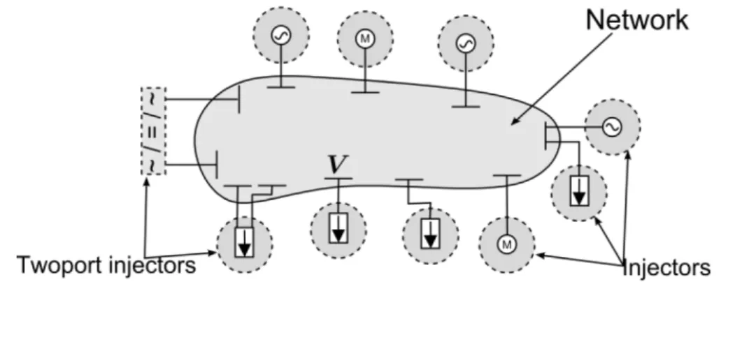
The dynamic simulation algorithm used in RAMSES belongs to the family of Domain Decomposition Methods (DDMs). The first step in applying a DDM is to select the domain partitioning. For the proposed algorithm, the electric network is first separated to create one sub-domain by itself. Then, each component connected to the network is separated to form the remaining N sub-domains. The components considered in this study refer to devices that either produce or consume power and can be attached to a single bus (e.g. synchronous machines, motors, wind-turbines, etc.) or on two buses (e.g. HVDC lines, AC/DC converters, FACTS devices, etc.). Hereon, the former components will be simply called injectors and the latter twoports. Components with three or more connecting buses can be treated as a combination of twoports.
The proposed decomposition can be visualized in Figure 1. The chosen scheme reveals a star-shaped, non-overlapping, partition layout. At the center of the star, the network sub-domain has interfaces with many smaller sub-domains; while, the latter interface only with the network sub-domain and not between them. Based on this partitioning, the sub-domain systems are modelled as follows.
The i-th injector is described by a system of Differential-Algebraic Equations (DAEs) [5]:
where xi is the state vector of the injector including the rectangular components of the injector currents (Ii), V is the vector of voltages through the network, and Li is a diagonal matrix with:
The network sub-domain is described by the algebraic equations:
acceleration techniques to achieve high simulation performance both in sequential and in parallel execution. This increased performance allows using detailed models to perform the above mentioned short and long-term dynamic simulations, while meeting the speed requirements. In the first stage of the integration, the new dynamic simulator will be used for the calculation and update of operation limits and to help alleviate network congestion problems. Later on, it is envisioned that its increased performance capabilities will enable real-time applications, like operator training or on-line contingency analysis.
2. Motivation
Due to geographic constraints, the HQ transmission system is characterized by long distances (more than 1,000 km) between the hydro-electric power generation and the main consumption centers. A large percentage of the 39,000 MW peak load is transferred over 735-kV, series-compensated, transmission lines. Owing to this structure (more than 11,000 km of 735-kV lines), the system is constrained by transient (angle) and long-term voltage stability. Moreover, as it is connected to its neighbors through DC lines or radial generators, its frequency dynamics after a severe power imbalance are carefully checked. Moreover as the system network is highly radial, changes in system topology result in significant differences in the dynamic response. As such, time domain dynamic simulations are required for each system configuration. Extensive dynamic simulations are performed to update the secure power transfer limits taking into account the N—1 security criteria, as well as to check the response of various stabilizing controls after severe disturbances.
Presently short term congestion is reduced by analyzing the predicted network and further optimizing the transmission limits. This is achieved using state estimator snapshots combined with the dynamic data to perform fully detailed simulation. In this context, computational speed and a robust algorithm are essential
The reduced system (5) is then solved using a sparse linear solver to acquire Vk. Finally, the latter is backward substituted in (4) and the variables xik of each injector sub-domain are computed.
The terms Ci Ai -1Bi have a predefined nonzero structure and are easy to compute. For example, if it is an injector attached to a single bus, this term consists of only four elements as the interfacing variables are the two injector current components and the two bus voltage components. Moreover, it modifies only four, already non-zero, elements of matrix D, thus retaining its original sparsity pattern. Similarly, a twoport contributes with nonzero elements as the interfacing variables are four current components and four bus voltage components (two for each of the connecting buses).
4. Acceleration techniques
In this section, the acceleration techniques (accel. techs.) sketched in Figure 2 are outlined. The first two acceleration techniques (A and B) target to decreasing the sequential execution time of the simulation. Thus, these techniques are designed to decrease the overall computational burden. On the contrary, the third technique is designed to distribute the computational burden among different computing units, thus decreasing the parallel execution time.
4.1. Localization (accel. tech. A)
The concept of localization results from the observation that in a large power system a disturbance may affect only a small number of components. This fact is exploited in three ways.
where D includes the real and imaginary parts of the bus admittance matrix, I=[I1,...,IN]T , and Ci is a trivial
matrix with zeros and ones whose purpose is to extract the current variables from xi.
An important benefit of this decomposition is the modelling modularity added to the simulation software and the separation of the injector modelling procedure from the solver. The predefined, standardized interface between the network and the injectors permits for the addition or modification of an injector in an easy way. For numerical simulation, the injector systems (1) are algebraized using a differentiation formula (e.g. trapezoidal formula, backward difference formula, etc). Next, at each discrete time instant tn, the N+1 sub-systems are solved using a Newton method. More precisely, at the
k-th Newton iteration the following N+1 linear systems
are solved:
where Ai is the i-th injector Jacobian matrix towards its own states and Bi towards the bus voltages.
For their solving, the interface variables between the sub-domains are updated using a Schur-complement approach [6] at each sub-domain Newton solution. In brief, a global reduced system is formulated by solving (4) towards the state corrections xik and replacing them in (3):
The technique employs simple and fast to compute metrics, originating from real-time digital signal processing, to classify each component into active or latent [7]. In brief, the variability of each injector’s per-phase apparent power (Si) is quantified by computing its
standard deviation (Sstd-i) over a moving time-window.
Standard deviations show how much variation or dispersion exists around the average.
Consequently, if Sstd-i is smaller than a chosen latency
tolerance (∈L), the i-th injector is considered to exhibit low dynamic activity and is declared latent. Thus, the full dynamic model (1) is replaced by the linear sensitivity-based (7). The average and standard deviations are computed using an efficient recursive formula as explained in [7].
Unlike the previous localization techniques, the use of latency can introduce some inaccuracy in the dynamic response. This inaccuracy is controlled by the choice of ∈L. Several studies on the HQ system have shown that a latency tolerance of ∈L=0.1MV A provides significant
speedup with very little inaccuracy. This will be further discussed in Section 5.
4.2. Time-scale decomposition (accel. tech. B)
When considering long-term dynamic simulations (e.g. for long-term voltage stability analysis), some fast components of the response may not be of interest and could be partially or totally omitted to provide faster simulations. This is achieved either by using simplified models (such as in the case of QSS simulations mentioned previously) or with a dedicated solver applying time-averaging [8].
While model simplification offers a big acceleration with respect to detailed simulation, some drawbacks exist. First, the separation of slow and fast components might not be possible for complex or black-box models. Furthermore, there is a need to maintain both detailed and simplified models. Finally, if both short and long-term evolutions are of interest, simplified and detailed simulations must be properly coupled.
At the same time, solvers using “stiff-decay” (L-stable) integration methods, such as Backward Difference Formula (BDF), with large enough time-steps can discard some fast dynamics. Such a solver, applied to a detailed model, can “filter” out the fast dynamics and concentrate on the average evolution of the system. The First, it is used within one discretized time instant solution
to stop computations of sub-domains whose models have already been solved with the desired tolerance. That is, after a solution of (3) and (4) has been obtained, the convergence of each sub-domain is checked individually. If the convergence criterion is satisfied, then the specific sub-domain is flagged as converged. For the remaining iterations of the current time instant, the sub-domain is not solved, although its mismatch, computed with (1) or (2), is monitored to guarantee that it remains converged. This technique decreases the computational effort within one discretized time instant without affecting the accuracy of the solution.
Second, each sub-domain is solved by a separate so-called Very DisHonest Newton (VDHN) method (i.e. a Newton method with infrequent update of the Jacobian matrix). Thus, the sub-system update criteria are decoupled and their local matrices (such as Ai, Bi, D), as well as their Schur-complement terms, are updated asynchronously. In this way, sub-domains which converge fast keep the same local system matrices for many iterations and even time-steps, while sub-domains which converge slower update their matrices more frequently. As with the previous technique, this one as well does not affect the accuracy of the solution.
Third, localization is exploited over several time steps by detecting, during the simulation, the injectors marginally participating to the system dynamics (latent injectors) and replacing their dynamic models (1) with much simpler and faster to compute sensitivity-based models. At the same time, the full dynamic model is used if an injector exhibits significant dynamic activity (active injectors). The sensitivity-based model used is derived from the linearized equations (4) when ignoring the internal dynamics, that is fi(xk-1,Vk-1)≈0, and solving
for the state variation :
The corresponding current variation is given by:
where Ei (similarly to Ci) is a trivial matrix with zeros and ones whose purpose is to extract the injector current variations from xik and Gi is a sensitivity matrix relating the current with the voltage variation.
these two parallelized steps have been found to sum up for almost 88% of the total computing time.
Finally, this acceleration technique maps the computational tasks to the available computing units. Thus, it can be combined with the accel. techs. A and B. Furthermore, due to the Schur-complement approach of treating the interface variables, the accuracy of the dynamic response is not affected by the parallelization procedure.
5. Experimental results
The HQ model used in this study includes 2565 buses, 3225 branches, and 290 power plants with a detailed representation of the synchronous machine, its excitation system, automatic voltage regulator, power system stabilizer, turbine and speed governor. Moreover, it has 4311 dynamically modeled loads (different types of induction motors, voltages sensitive loads, etc.). In the long-term the system evolves under the effect of 1111 Load Tap Changer (LTC) devices, 25 Automatic Shunt Reactor Tripping (ASRT) devices [9], as well as OvereXcitation Limiters (OXL). The resulting model has differential-algebraic states. Using the method described in Section 3, the system is decomposed into the network sub-domain, including buses, and the N = 4601 injectors. In the following example, the disturbance consists of a bus-bar fault lasting six cycles (at 60 Hz) that is cleared by opening two 735-kV lines. Then, the system is simulated over an interval of 240 s.
As a benchmark, the simulation is performed by solving (3) and (4) together, using a single VDHN method. For this, the Jacobian matrix is updated every 5 iterations until convergence and a constant time-step size of one cycle is used. This benchmark solution will be referred to as Integrated.
For the accel. tech. A, two latency tolerances of ∈L = 0 MV A (fully accurate simulation) and ∈L = 0.1 MV A are considered. For time-scale decomposition (accel. tech. B), a time-step size of one most significant advantage of this approach is that it
processes the detailed, reference model. Furthermore, this technique allows combining detailed simulation in the short term by limiting the step size, and time-averaged in the long term by increasing it.
As power systems are described by hybrid models, an important consideration when increasing the time-step size is the treatment of the discrete events. In the context of time-averaging an ex-post treatment of discrete events can be used as detailed in [8]. Summarizing the scheme used, at any time t a time-step h is taken and the corresponding state vector x(t+h) is computed. Then, the system is checked for any violated discrete change conditions. If it is detected that a discrete event has occurred within the time-step, the DAEs are changed accordingly and the step t → t+h is repeated to compute a new state vector x(t+h). This technique employs “warm-start”, that is the previously computed states are used as initial values to solve the updated equations, thus significantly reducing the computational cost. This procedure is repeated, updating the state vector, until no more discrete conditions are violated or a maximum number of repetitions is reached. This yields the final state vector for the current step.
4.3. Parallel computing (accel. tech. C)
One of the principle reason for employing DDMs is the parallelization potential inherent to them. Thus, the proposed algorithm is implemented using shared-memory parallel programming techniques to take advantage of the computational resources available in multi-core computers. This is achieved by parallelizing the independent calculations relative to the sub-domains. Two steps of the presented algorithm are parallelized. First, the algebraization of the injector DAE systems (1) to get the corresponding non-linear algebraized systems (4), the linearization of the latter to calculate the individual Jacobian matrices, the factorization of the matrices and the calculation of the terms Ci Ai -1Bi and
Ci Ai -1fi. Second, the solution of the linearized systems (4) to compute the state corrections and the convergence check of the injector DAE models. For the HQ system,
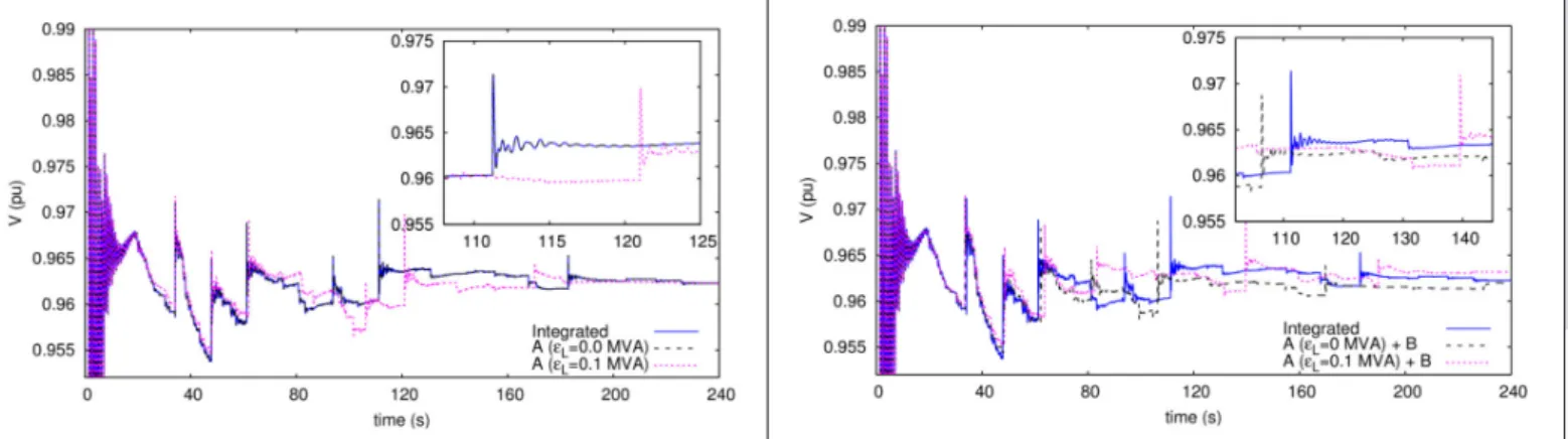
Figure 3 Voltage evolution at 735-kV bus close to the fault
enough to shift its action in time. However, in all five simulations shown in Figure 3 Voltage evolution at 735-kV bus close to the fault with accel. tech. A, the same number of ASRT actions take place (six), for the same devices and with the same sequence. Moreover, in all simulations, the final voltage is reached before t=200 s and the final voltage values are the same (with an error margin of 0.005 pu). Based on these observations, all five simulation responses are deemed to be correct.
5.2. Performance
Table I Sequential and parallel performance of algorithm shows the sequential (on 1 core) and parallel (up to 24 cores) performance of the DDM-based algorithm compared to the benchmark Integrated algorithm. First, the sequential speedup achieved by the accel. techs. A and B is seen at the first row of the table (1 core). It can be seen that compared to the Integrated, the DDM-based algorithm can achieve a speedup of 2.2 times without any inaccuracy, and 6.8 times with some acceptable inaccuracy affecting the system response. This increased performance is critical when a contingency is simulated on a single processing unit, or for analyzing several contingencies in parallel, each on a single processing unit.
The parallel performance of the DDM-based algorithm is clearly seen from the next rows of the table. This technique can be combined with A and B, without modifying the simulation response. It can be seen that the DDM-based algorithm can achieve a speedup of 11.5 times faster execution without any inaccuracy, and 26.3 times with some acceptable inaccuracy.
cycle is used for the first 15 s (short term) and 0.05 s for the remaining simulation interval. To assess the parallel performance of the algorithm (accel. tech. C), a 24-core AMD Opteron Interlagos desktop computer and the OpenMP application programming interface were used [10].
5.1. Dynamic response
The plots of Figure 3 Voltage evolution at 735-kV bus close to the fault with accel. tech. A and Figure 4 Voltage evolution at 735-kV bus close to the fault with accel. techs. A and B show the voltage evolution at a 735-kV bus close to the fault. In the short-term (up to t=20 s) all simulations, for this case, provide the same, accurate, response. From Figure 3 Voltage evolution at 735-kV bus close to the fault with accel. tech. A, it can be seen that using accel. tech. A with ∈L = 0 MV A leads to completely accurate
simulation response as the curve is indiscernible from the benchmark throughout the whole simulation. When latency is used (∈L = 0.1 MV A), the system response is
modified and the switching times of some ASRT devices are shifted. Similarly, from Figure 4 Voltage evolution at 735-kV bus close to the fault with accel. techs. A and B it can be seen that when accel. tech. B is used, the system response is also modified with the ASRT device actions being further shifted in time.
It must be noted that, although the difference seems large at first glance, it is considered acceptable by the HQ engineers. In fact, the voltage monitored by the ASRT device evolves marginally close to the triggering threshold, and a small difference in system trajectory is
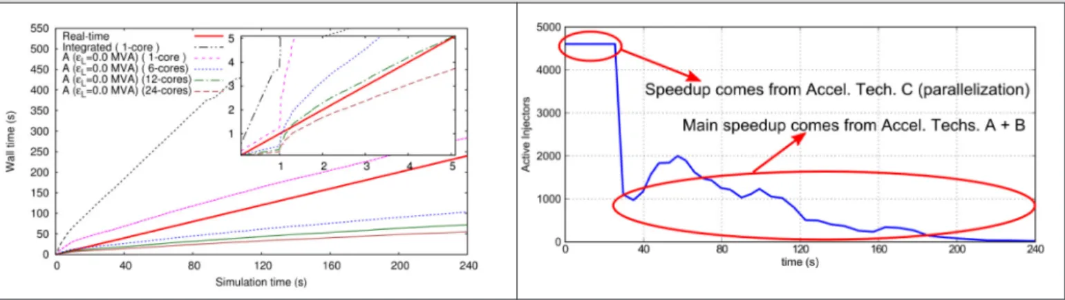
Figure 5 Real-time performance of algorithm with accel. techs. A (∈L = 0 MV A) and C
Figure 6 Number of active injectors with accel. techs. A (∈L = 0 .1MV A), B, and C
Execution time (s) / Speedup compared to Integrated
Cores Integrated A (∈L= 0 MVA) A (∈L= 0.1 MVA) A (∈L= 0) +B A (∈L= 0.1) +B
1 630 / 1.0 284 / 2.2 191 / 3.3 130 / 4.8 93 / 6.8
2 - 168 / 3.8 131 / 4.8 77 / 8.2 61 / 10.3
6 - 103 / 6.1 96 / 6.6 48 / 13.1 44 / 14.3
12 - 73 / 8.6 68 / 9.3 34 / 18.5 32 / 19.7
24 - 55 / 11.5 53 / 11.9 26 / 24.2 24 / 26.3
times, when some acceptable inaccuracy is allowed. Nevertheless, the dynamic responses have been found to be acceptable.
Additionally, it was shown that when RAMSES is executed on a 24-core, shared-memory, desktop computer, it can provide faster than real-time, look-ahead, simulations. Finally, it was shown that the acceleration techniques used in RAMSES complement each other by providing speedup at different segments of the simulation.
Based on these very promising results, HQ is integrating RAMSES into their simulation environment. The performance gains will result in better system understanding and further limit optimisation. RAMSES’ performance gains will be critical in an on-line DSA system.
7. References
[1] L. Loud, S. Guillon, G. Vanier, J. A. Huang, L. Riverin, D. Lefebvre, and J. C. Rizzi, “Hydro-Québec’s challenges and experiences in on-line DSA applications,” in Proc. of 2010 IEEE PES General Meeting, 2010.
[2] T. Van Cutsem, M. E. Grenier, and D. Lefebvre, “Combined detailed and quasi steady-state time simulations for large-disturbance ana-lysis,” Int. J. Electr. Power Energy Syst., vol. 28, no. August, pp. 634– 642, 2006.
[3] P. Aristidou, D. Fabozzi, and T. Van Cutsem, “Dynamic Simulation of Large-Scale Power Systems Using a Parallel Schur-Complement-Based Decomposition Method,” IEEE Trans. Parallel Distrib. Syst., vol. 25, no. 10, pp. 2561–2570, Oct. 2013.
[4] P. Aristidou and T. Van Cutsem, “Algorithmic and computational advances for fast power system dynamic simulations,” in Proc. of 2014 IEEE PES General Meeting, 2014.
[5] P. Kundur, Power system stability and control. McGraw-hill New York, 1994.
[6] Y. Saad, Iterative methods for sparse linear systems, Second. Society for Industrial and Applied Mathematics, 2003.
[7] P. Aristidou, D. Fabozzi, and T. Van Cutsem, “Exploiting Localization for Faster Power System Dynamic Simulations,” in Proc. of 2013 IEEE PES PowerTech conference, 2013.
[8] D. Fabozzi, A. S. Chieh, P. Panciatici, and T. Van Cutsem, “On sim-plified handling of state events in time-domain simulation,” in Proc. of 17th Power System Computational Conference (PSCC), 2011. [9] S. Bernard, G. Trudel, and G. Scott, “A 735 kV shunt reactors
auto-matic switching system for Hydro-Quebec network,” IEEE Trans. Power Syst., vol. 11, no. 4, pp. 2024–2030, 1996.
[10] R. Chandra, Parallel programming in OpenMP. Morgan Kaufmann, 2001.
Figure 5 shows the shows the real-time performance of the parallel DDM-based algorithm with accel. techs. A (∈L = 0 MV A) and C. When the execution (wall) time
curve is above the real-time line, then the simulation is lagging; otherwise, the simulation is faster than real-time and can be used for more demanding applications, like look-ahead simulations, training simulators, or hardware/software in the loop. On the HQ power system, the algorithm, implemented in RAMSES, performs faster than real-time for each time step when executed on 24 cores.
Finally, Figure 6 shows the number of active injectors during the fastest simulation with accel. techs. A (∈L = 0.1 MV A), B, and C. It can be seen that in the
short-term all injectors remain active, while a small time-step size is used, thus the main speedup in this period comes from the parallelization of the algorithm. In the long term, a bigger time-step size is used and, as the electromechanical oscillations fade, the injectors start switching to latent and decrease the computational burden of treating the injectors. Hence, in this part of the simulation, the main source of acceleration are accel. techs. A and B. Consequently, the accel. techs. of Figure 2 Acceleration techniques used in RAMSES complement each other as they perform better at different parts of the simulation.
6. Conclusion
In this paper, the DDM-based algorithm implemented in the dynamic simulator RAMSES has been presented, along with the acceleration techniques used to increase the performance of both sequential and parallel execution. RAMSES exploits the localized response of power systems to disturbances and the time-scale decomposition of dynamic phenomena to provide sequential acceleration when the simulation is performed on a single processing unit. In addition, when more computational units are available, the parallelization potential of DDMs is exploited providing parallel acceleration.
Furthermore, the algorithm and acceleration techniques have been tested on a real-life HQ system model and the accuracy of dynamic response, the sequential, parallel, and real-time performance have been evaluated. It was shown that RAMSES can provide high-performance dynamic simulations with speedups of up to 11.5 times when fully accurate simulations are required, or 26.3
in 1985 and 1988, respectively, and the Ph.D. degree from McGill University in 1996. He has been with Hydro-Quebec research institute, IREQ, since 1994, where he is involved with dynamic and voltage security assessment and congestion management.
Thierry Van Cutsem graduated in Electrical-Mechanical Engineering from the University of Liège, Belgium, where he obtained the Ph.D. degree and he is now adjunct professor. Since 1980, he has been with the Fund for Scientific Research (FNRS), of which he is now a Research Director. His research interests are in power system dynamics, stability, security, monitoring, control and simulation. He has been working on voltage stability in collaboration with transmission system operators from France, Canada, Greece, Belgium and Germany. He is a fellow of the IEEE and Past Chair of the IEEE PES Power System Dynamic Performance Committee.
8. Biographies
Petros Aristidou obtained his Diploma in Electrical and Computer Engineering from the National Technical University of Athens, Greece, and his Ph.D. in Engineering Sciences from the University of Liège, Belgium, in 2010 and 2015, respectively. He is currently a postdoctoral researcher at the Swiss Federal Institute of Technology in Zürich (ETH Zürich). His research interests include power system dynamics, control, and simulation.
Simon Lebeau received his B.Eng. degree in Electrical Engineering from École Polytechnique, Montréal, in 2001. He is with the Hydro-Québec TransEnergie Division where is involved in operations planning for the Main Network using dynamic simulations.
Lester Loud received, in electrical engineering, the B.Eng. and M.Eng. degrees from Concordia University