What is the Effect of Foreign Direct Investment
on the Host Economy?
An Analysis For Developed Countries with a Focus on Canada
By:
Deirdre Lynn Morris
Supervisor:
Professor Benoît Perron
Département de sciences économiques
Faculté des arts et des sciences
Université de Montréal
August 2008
Abstract
There has been debate in Canada over what stance our country should take with regards to the regulation of FDI. This paper examines one important aspect of this debate.
Firstly, academic literature on this topic is reviewed and it is found that the results are mixed.
For the empirical analysis, this study looks at whether the data suggests FDI brings with it a positive externality to the host country using a growth accounting
framework. The analysis starts with an examination of Canadian data using both OLS and TSLS estimation. Next, international data is used to further investigate the question. Two different multi-country data sets are assembled using a selection of OECD countries and two different time periods. For each set, the data is pooled and the fixed effects and Arellano-Bond estimators are used.
The OLS regressions using Canadian data that include between two and five lags of the growth rate of FDI stock showed that same-period growth in FDI stock has a significantly positive effect on economic growth. The other coefficients associated with FDI are not statistically significant – with most being positive and a few being negative. This analysis was not able to produce a decisive result regarding externalities in the host economy due to increases in the stock of FDI.
1) Abstract Pg. 1
2) List of Tables Pg. 3
3) Section 1: Introduction Pg. 4
4) Section 2: Background Information Pg. 6 5) Section 3: Literature Review Pg. 8 6) Section 4: Theoretical Framework Pg. 13 7) Section 5: Empirical Analysis Pg. 15
8) Section 6: Conclusion Pg. 27
9) Bibliography Pg. 29
Table 1: Unrestricted OLS Estimation – Canadian Data Set Pg. 16 Table 2: Restricted OLS Estimation – Canadian Data Set Pg. 17 Table 3: Unrestricted and Restricted TSLS Estimation– Canadian Data Set Pg. 18 Table 4: Unrestricted OLS Estimation – International Data Set #1 Pg. 22 Table 5: Restricted OLS Estimation – International Data Set #1 Pg. 23 Table 6: Unrestricted and Restricted OLS Estimation
– International Data Set #2 Pg. 24
Table 7: Arellano-Bond – International Data Set #2 Pg. 25
Section 1: Introduction
There has been debate in Canada and in many other countries over the
(FDI).
Those in favor of increasing the promotion of FDI argue that the host country benefits from both the new capital as well as positive spillovers that the presence of the new capital produces.
Assuming the foreign firms that invest in the local economy have a technological advantage of some sort, there are a number of different channels through which domestic firms are thought to benefit by means of positive spillovers.
As is explained by Görg and Greenaway (2002), a possible channel is one in which domestic firms are thought to ‘imitate’ the technology used by the foreign companies. This would lead to technological improvements for local companies by means of indirect transfers as they try to incorporate as much as possible the new
methods into their own production. Another channel is ‘skill acquisition’ where domestic workers may benefit from the employee training by technologically advanced companies – this would lead to increased human capital in the host country. A third channel is ‘competition’. With the entry of advanced foreign companies, local companies are forced to compete and therefore are thought to become more efficient.
On the other side of the debate, it is argued that there will be future outflows of profits and a decrease in domestic control of assets. Another possible argument, as Görg and Greenaway suggest, is that the ‘competition’ spillover channel mentioned above could decrease the productivity of domestic firms – the entry of a foreign firm with “lower marginal costs than” domestic competitors could “force domestic firms to reduce production and move up their average cost curve” if the foreign firm causes a shift in demand from domestic firms towards itself. (Görg and Greenaway (2002, 2-3))
At the 2007 annual general meeting of the Canadian Chamber of Commerce (2007), a resolution entitled “Attracting Foreign Direct Investment to Canada” was passed. The document calls for the Canadian government to “send a clear and positive message to foreign investors that Canada wants inbound investment through a proactive investment strategy and promotion campaign”. On the other hand, opponents of FDI call for tighter restrictions. Should host countries take the advice of the proponents or the opponents of FDI?
This paper examines only one important aspect of this question – it looks at
whether an increase in the stock of FDI creates positive externalities for the host economy. The framework of the empirical study presented is a growth accounting model that uses both Canadian and international data. Ordinary least squares (OLS) and two stage least squares (TSLS) estimation is used with the Canadian data. The fixed effects and the Arellano-Bond estimators are used with the pooled international data, which is taken from a selection of OECD countries.
The remainder of this paper is structured in the following way: Section 2 discusses background information important to the subject of FDI. Section 3 is a review of academic literature examining similar topics. Section 4 develops the theoretical framework used while Section 5 presents the empirical analysis. Finally, Section 6 concludes.
Section 2: Background Information
FDI is a component of a country’s international investment position. A country’s net international investment position is “the difference between total financial assets and total financial liabilities”.(Statistics Canada (2008)) Both financial assets and financial liabilities are made up of three components: direct investment, portfolio investment and other investment. (Statistics Canada (2008)) For example, FDI is a financial liability for
the country in which the investment is being made and an asset for the country from which the investment originates (Direct Investment Abroad).
The way in which FDI differs from the other components of international investment, such as portfolio investment, is that with FDI, there is a “lasting interest”. (IMF (2003, 6)) The International Monetary Fund (IMF) defines FDI as: “A category of international investment that reflects the objective of a resident in one economy (the direct investor) obtaining a lasting interest in an enterprise resident in another country.” (IMF (2003, 6)) The IMF’s definition further explains that “a direct investment
relationship is established when the direct investor has acquired 10 percent or more of the ordinary shares or voting power of an enterprise abroad.” (IMF (2003, 6-7))
The world has experienced large increases in FDI in the last two decades. “In the 1990s [FDI increased] at rates well above those of global economic growth or global trade.” (IMF (2003, 9)) These increases have no doubt been made possible by the regulatory changes that have occurred – both national and international. The United Nations Conference on Trade and Development(UNCTAD) started gathering data pertaining to FDI regulations in 1991 and they report that “between January 1991…and December 2002, a total of 1,641 measures were introduced by 165 countries, 95 percent of them representing changes more favourable to FDI.” (UNCTAD (2003)) The nature of these measures range from increased protection for the investors, to liberalization of rules governing entry of foreign investors to measures that are “promotional in nature,
including incentives”. (UNCTAD (2003)) Besides these changes in national regulations, there has also been encouragement of FDI on an international level through bilateral investment treaties (BITs) and double taxation treaties (DTTs), which are established “for the avoidance of double taxation on income and capital in the partner countries”.
(UNCTAD (2003))
In Canada, there have been many changes to the rules governing FDI in the last half century. Due to growing concern over FDI in the late1960s and early1970s, the Foreign Investment Review Agency (FIRA) was established to regulate new FDI. (Gellaty (2006, 3.10-3.11)) Then, in the 1980s, regulations governing FDI were
liberalized and in 1985, the FIRA was replaced with Investment Canada whose purpose was to promote FDI in Canada. With the implementation of the Canada-U.S. Free Trade
Agreement (CUFTA) and then the North American Free Trade Agreement (NAFTA), FDI in Canada was further liberalized. (Gellaty (2006, 3.11)) World Trade Organization (WTO) rules also required increased liberalization. (Holden (2007, 2-3))
Today, the rules governing FDI vary widely from country to country. In Canada, regulations differ depending on whether the country is a WTO member and if the investment is being made in one of the specific protected sectors – namely, “uranium production, financial services, cultural industries, or transportation services”. (Holden (2007, 3)) If the investment is being done by a WTO member and it is a direct
acquisition, it is reviewed if it is greater than an amount that is calculated with a “pre-determined formula based on growth in Canada’s gross domestic product (GDP)” – in 2007, this amount was $281 million. If the investment is being done by a WTO member and it is an indirect acquisition – “one in which the investor buys shares of a company that is incorporated outside Canada but owns subsidiaries in Canada” (Holden (2007, 2)) – there is no review of the investment, but it is “subject to a requirement to provide notification”. (Holden (2007, 2)) The regulations governing non-WTO members are much stricter. (Holden (2007, 2))
Section 3: Literature Review
The conclusions of the available literature on the effects of FDI on economic growth are mixed – they range from suggesting that there is not a significant relationship between the two to stating there is a significantly positive one. Here several studies with varying results are reviewed.
Maria Carkovic and Ross Levine (2002), in Does Foreign Direct Investment
Accelerate Economic Growth?, claim that “FDI inflows do not exert an independent
influence on economic growth”. (Carkovic and Levine (2002, 219))
For their investigation, they first use OLS estimation to regress economic growth on inflows of FDI as a share of GDP and other control variables using cross-sectional
data – with the data being averaged over the 36 year period from 1960 to 1995 and including both wealthy and poor countries. Secondly, they use a Generalized Method of Moments (GMM) dynamic panel estimator with the data averaged over five-year periods. A number of regressions are performed for each model taking different control variables into account each time.
For the regressions using the cross-sectional data, the authors report that “FDI does not enter these growth regressions significantly”. (Carkovic and Levine (2002, 204)) For the dynamic panel model, the coefficient for FDI is positive and significant in three of the seven regressions.
Bruce A. Blonigen and Miao Grace Wang (2004) argue in their article,
Inappropriate Pooling of Wealthy and Poor Countries in Empirical FDI Studies, that
growth accounting models testing for the effect of FDI on economic growth produce misleading results due to the pooling of rich and poor countries.
One of the sections in their study examines the effect of FDI on economic growth using a growth accounting model that allows the coefficients for poor and wealthy countries to differ. In this section they use both seemingly unrelated regression (SUR) estimation and random effects estimation. The panel data covers the period from 1970 to 1989 and is averaged over two ten year periods. The variable for FDI is the sum of FDI flows during each of the two periods.
First, using SUR estimation, a base regression with wealthy and poor countries pooled together, was performed. It was found that the coefficient associated with FDI is positive and not statistically significant. Secondly, the sample of countries was divided into two groups – developed countries (DCs) and least developed countries (LDCs) – and a dummy variable for the LDCs was interacted with the explanatory variables. The results showed that for the LDCs, FDI had a significantly positive effect on economic growth when educational attainment reached a certain level. For the DCs, a significant
relationship between FDI and economic growth was not found.
Similar result were found when using the random effects estimator – for LDCs the effect was positive and significant after a certain educational attainment was achieved and for DCs the authors report that there is not a statistically significant relationship between FDI and economic growth.
Conflicting results were presented by Benhua Yang (2007) in FDI and growth: a
varying relationship across regions and over time. This study also examines the effect of
FDI on economic growth by regressing economic growth on FDI inflows as a percentage of GDP and other control variables; however, here the author allows the coefficients for the explanatory variables to differ for up to seven different regions.
The study used panel data – a large sample of countries for the time period between 1973 and 2002, with the data averaged over five year periods.
Firstly, a base case – for which the regions were not accounted for separately – was estimated. In this first regression, the author finds that the coefficient on the FDI variable is positive and not statistically significant.
After this, the effect of FDI on economic growth was allowed to differ between different groups of countries – first between OECD countries and developing countries and second between OECD countries and six other regions. Unlike the previous study, the coefficient associated with FDI for the OECD countries is positive and significant.
Finally, the data is divided into two fifteen-year periods in order to examine whether the effect has changed over time. For the OECD countries, the coefficient for the first period (1973-1987) is negative and insignificant and the coefficient for the second period (1988-2002) is positive and significant.
A test for Granger causality is used by Jong Il Choe (2003), in Do Foreign Direct
Investment and Gross Domestic Investment Promote Economic Growth?, to examine the
relationship between FDI and economic growth.
The author used a sample of 80 countries that includes both developed and
developing countries. Firstly, the entire sample was used. This was followed by a second sample that had the outliers removed. In this case, 'outliers' is defined as “observations where the distance between the individual residual and the mean of the residuals exceeds the standard deviation of the residuals by more than a factor of three”. (Choe (2003, 51)) The time period covered was from 1971 to 1995 and the data was averaged over five-year periods.
Choe tested whether FDI Granger-causes economic growth as well as whether economic growth Granger-causes FDI – with the variable representing FDI being the ratio of FDI inflows to GDP. For the first sample, it was found that FDI does indeed
Granger-cause economic growth and that economic growth Granger-causes FDI. When the second sample was used, the author found that FDI does not Granger-cause economic growth and that economic growth does Granger-cause FDI.
The author concludes that “causality seems to run in either direction, but the effects are more apparent from growth to FDI than from FDI to growth”. (Choe (2003, 52))
Robert Lensink and Oliver Morrissey (2006) also examine the relationship between FDI and economic growth; however, they add another aspect to the analysis – volatility.
In their paper, Foreign Direct Investment: Flows, Volatility, and the Impact on
Growth, they use a sample of 87 countries that includes both developed and developing
countries and they use both cross-sectional as well as panel data. The cross sectional data regresses average per capita economic growth between 1970 and 1998 on the average ratio of FDI inflows to GDP (GFDI) over the period from 1975 to 1997, on the volatility of FDI which “is measured by taking the standard deviation of errors from the
autoregressive equation for GFDI with lagged values (three years) and a time trend” (Lensink and Morrissey (2006, 484)), and on other control variables. The panel data is divided into three periods (1970–80, 1980–90, and 1990–97) and period averages are used in the model.
First, OLS estimation was used for the cross-sectional data and it was found that the coefficient for FDI was positive and significant while the coefficient for the volatility of FDI was negative and significant. Secondly, two-stage least squares estimation was used in order to deal with endogeneity and the results support those found in the first
regression. The panel data was estimated using the fixed effects estimator and the authors report that the results are similar to the previous results except that “evidence for a
positive effect of FDI is not robust: the coefficient is insignificant”. (Lensink and Morrissey (2006, 486))
Peter Blair Henry (2007), in his recent work on capital account liberalization, makes the observation that according to economic theory, capital account liberalization will not lead to a permanent increase in economic growth but rather a temporary increase in growth and a permanent increase in the level of GDP. He argues that many researchers have not been testing what the theory predicts since often cross-sectional data is used to
test the effect of capital account liberalization on GDP growth averaged over fifteen years and therefore the test looks for a permanent increase in GDP growth rather than a
temporary one. As is clear from the discussion above, the same problem exists for studies that focus on FDI. It follows from Henry’s argument that when studying the effect of FDI on economic growth, the model should be designed to test for a temporary and not a permanent effect. Since a return to the steady state is not instantaneous, however, the correct length of the temporary effect is not completely clear. Henry suggests that “a short window of five years or less is theoretically appropriate”. (Henry (2007, 32))
Using Henry’s five-year criteria, among the studies described above, it is
Carkovic and Levine (2002) (when using their panel data), Yang (2007) and Choe (2003) who test for a temporary effect of FDI on economic growth.
All of the studies reviewed here use various different variables to account for FDI, but none of them use increases in the stock of FDI. This paper differs in this respect. In the following sections, a model that tests for a temporary effect of the growth of FDI stock on economic growth is developed and analyzed.
Section 4: Theoretical Framework
The question being asked in this analysis is whether there is an externality
associated with FDI – the model developed below is designed to determine if FDI has an effect on total factor productivity.
Following Ann Harrison (1996), the model used in this analysis starts with a Cobb-Douglas production function of the following form:
Y
it= A
itF (K
it, L
it) = A
itK
itαL
itλ(1)
where
Y
it = total output for country i in year tK
it = total capital stock in country i in year tL
it = total hours worked in country i in year tA
it = total factor productivity for country i in year tTaking logarithms and time derivatives of Equation (1) gives:
Δln Y
it= Δln A
it+ αΔln K
it+ λΔln L
it(2)
The first term,
Δln A
it , represents technological change and in this model will bewritten as the sum of two components. The first is technological change due to FDI. For this variable the change in the log of FDI stock,
Δln FDI
it , is used as a proxy variable.The second is a disturbance term,
e
it , which captures other sources of total factorproductivity. Breaking
Δln A
it into its components and substitutingα
withβ
1andλ
with
β
2gives:Δln Y
it= β
1Δln K
it+ β
2Δln L
it+
β
3Δln FDI
it+
e
it(3)
For the model using international data, a country specific term,
f
i , that is constantover time is also included to account for differences between countries that are not modeled:
Δln Y
it=
β1Δln K
it+ β
2Δln L
it+
β
3Δln FDI
it+
f
i+ e
it(4)
It should be noted that this model imposes the restriction that the coefficients are equal across all countries in the sample being used. Therefore, for the multi-country data sets used in Section 5, even though the samples include only developed countries, this may affect the results since some countries are more advanced than others.
The main coefficient of interest for this study is the coefficient associated with FDI,
β
3. If the accumulation of the stock of FDI in the host country produces a positiveexternality – for example, technological advancements –
β
3 will be positive and if aSection 5: Empirical Analysis
This section is divided into two parts – Part 1 uses Canadian data and Part 2 international data. Both use the theoretical framework developed in the previous section to test for the presence of an externality in the host country caused by increases in the stock of FDI.
Part 1 – Canadian Data:
Data and Empirical Model
This section looks at the Canadian experience with FDI between 1962 and 2006. For income, capital and labour a special series created by Statistics Canada, which is in index form and covers the business sector, is used. The variable representing income is “a chained Fisher quantity index of GDP … at basic prices”, the variable representing capital is a “chained-Fisher aggregation of capital stocks using the cost of capital to determine weights”, and the variable representing labour is a “chained-Fisher aggregation of hours worked of all workers, classified by education, work experience, and class of workers (paid workers versus self-employed and unpaid family workers) using hourly compensation as weights.” These indexes are used to calculate the annual growth rate of Y, K and L. For the variable representing FDI, this paper differs from the studies
presented in the literature review by using the growth rate of the stock of FDI, which is calculated using data from Statistics Canada.
Following the discussion above and the theory developed in Section 4, Equation 5 (below) will be the first considered. Of course, since only one country is represented in
the data, the variable representing the country specific effect,
f
i , as well as the countrysubscripts are removed.
g
yt= α+ β
1g
kt+ β
2g
Lt+
β
3g
fdit+ e
t(5)
where
g
xt = the growth rate of variable x for period tBoth OLS and TSLS estimation are used.
Expected Results
According to the theory elaborated in Section 4, the coefficient on the percentage change in FDI stock will be positive if the accumulation of the stock of FDI results in positive externalities such as an increase in technology for the host country and will be negative if increased FDI produces negative externalities within the host economy.
And, of course, percentage increases in L and K are expected to have positive impacts on GDP growth.
Results
The results of the estimation of Equations 5 using OLS and Newey-West
heteroskedasticity and autocorrelation consistent (HAC) standard errors are presented in Table 1. The coefficient for the growth rate of FDI stock is positive but not statistically significant while the coefficients for the growth rates of K and L are significant, using a 10% level of significance, and the signs are positive as expected.
Table 1: Unrestricted OLS Estimation – Canadian Data Set
Coefficient Stand. Error t-Statistic
g
k 0.2077 0.1068 1.9451g
L 0.8261 0.1837 4.4977However, the coefficient for the growth rate of K is smaller and the coefficient for the growth rate of L is larger than commonly found. Therefore, a Wald test is used to test the restriction of constant returns to scale
(β
1 +β
2 =1)
to determine if imposing such arestriction in the regression may be beneficial. The p-value for the test is 0.8095 and therefore, the null hypothesis that
β
1 +β
2 =1 is clearly not rejected. Based on this result,Equation 6 (below), which imposes the stated restriction, is estimated. The results are in Table 2. They are similar to those found for the unrestricted case, however, the
coefficient for
g
kis not statistically significant when the restriction is imposed.g
yt= α+ β
1g
kt+ (1-β
1) g
Lt+
β
3g
fdit+ e
t(6)
Table 2: Restricted OLS Estimation – Canadian Data Set
Coefficient Stand. Error t-Statistic
g
k 0.1892 0.1366 1.3853g
L 0.8108 0.1366 5.9363g
fdi 0.0397 0.0675 0.5872One aspect of concern regarding Equations 5 and 6 is that only same-period effects of FDI growth on the growth of GDP are accounted for. Therefore, equations with various numbers of lags of
g
fdi were examined and sequential tests were performed in order to determine the optimal number of lags. To start, five lags ofg
fdi were included and a test on the coefficient forg
fdit-5 was performed. The null hypothesis that thiscoefficient is equal to zero was not rejected; therefore,
g
fdit-5 was removed and aregression with four lags of
g
fdi was performed. The coefficient forg
fdit-4 was then tested.This procedure was to continue until either the last lag included was statistically
significant or there were no more lags remaining. For both the restricted and unrestricted models, all lags were removed – it was determined that zero lags is optimal. (It should be
noted, however, that growth of FDI stock had a significantly positive same-period effect on economic growthin the models that included between two and five lags of
g
fdi.)Another concern for the OLS estimations above is that some or all of the
independent variables may be endogenous – a Hausman test is used to examine this issue. As the test dictates, the reduced form equation for each variable being tested (
g
L,g
k andg
fdi)was estimated – with lagged values of the variable being considered used asinstruments – and the residuals for each of the three regressions were saved. The original equation, Equation 5, was then estimated with the three sets of residuals included as regressors. The p-value for the coefficient associated with the residuals of the reduced form for
g
L is 0.5604, forg
k is 0.2425 and forg
fdi is 0.3358. Therefore, for each variable, we do not reject the null hypothesis that it is exogenous.Next, the same equations are re-estimated using TSLS. The restriction of constant returns to scale was tested using the unrestricted equation and the null hypothesis that the coefficients associated with capital and labour sum to one was not rejected with a p-value of 0.1870; therefore, the restricted equations are also presented below. The results for the unrestricted and restricted equations are in Table 3.
The same sequential procedure was followed as for the OLS estimation to determine the number of lags to include and it was found that the optimal number was again zero. The results are robust in terms of the number of lags of
g
fdi included.Table 3: Unrestricted and Restricted TSLS
Estimation– Canadian Data Set Unrestricted Restricted
g
k 0.1708 (0.2196) [0.7778] 0.3372 (0.1795) [1.8783]g
L 0.4869 (0.2483) [1.9605] 0.6628 (0.1795) [1.4690]g
fdi -0.0469 (0.1943) [-0.2413] -0.1873 (0.1905) [-0.9831]The results of the unrestricted equation are not as expected. The coefficient for
g
L is the only one that is significant at the 10% significance level. Furthermore, themagnitude of the coefficients for
g
L andg
k are not close to what is commonly found in growth accounting models.The results are quite different for the restricted model. The coefficients for
g
L andg
k are in their expected range and they are statistically significant using a 10%significance level. The coefficient associated with FDI stock is not statistically significant.
Overall, after examination of the Canadian data, this analysis does not allow a decisive conclusion to be made regarding externalities in the host economy due to increases in the stock of FDI. The growth of FDI stock had a significantly positive same-period effect on economic growthin the models that used OLS estimation and that included between two and five lags of
g
fdi.
The coefficients associated with FDI in the other regressions were not statistically significant.Next, further investigation of the effect of FDI on the host economy is pursued using international data.
Part 2 – International Data:
Empirical Model
Pooled data, which includes a selection of OECD countries, is used in this
analysis. Due to data constraints, two sets of data – which differ in terms of the countries included, the time period examined and one of the variables employed for estimation – are used. Therefore two equations are considered – they are shown below. As seen in Equation 10, which makes use of the second set of international data, the ratio of investment to GDP is used as a proxy for the stock of capital since this variable was not available for the time period examined. In order to use this proxy variable, the hypothesis – which is consistent with the neo-classical growth model in the steady state – that investment is proportional to the stock of capital is made.
Δln Y
it=
β1Δln K
it+ β
2Δln L
it+
β
3Δln FDI
it+
f
i+ e
it(9)
Δln Y
it=
β1Δ(INV/GDP)
it+ β
2Δln L
it+
β
3Δln FDI
it+
f
i+ e
it(10)
where
Y
= GDPL
= total hours workedK
= the stock of capital(INV/GDP)
= investment as a share of GDPFDI
= the stock of foreign direct investmentf
= a country specific effect (which is constant over time)e
= error term
Since the country specific terms are unknown, fixed effects estimation is used to remove these terms from the estimated model. Therefore, the actual models estimated are such that the variables in Equations 9 and 10 are time-demeaned: (Wooldridge (2006, 485-486)
. . . . . . . . . .
Δln Y
it=
β1Δln K
it+ β
2Δln L
it+
β
3Δln FDI
it+ e
it(11)
. . . . . . . . . .
Δln Y
it=
β1Δ(INV/GDP)
it+ β
2Δln L
it+
β
3Δln FDI
it+ e
it(12)
. .where X signifies that the variable has been time-demeaned:
. . __
X
it =X
it– X
iBecause the time-demeaning removes the country specific effects, country specific control variables common to growth accounting such as GDP at the start of the period or secondary school enrollment at the start of the period are not explicitly included – they are in fact included in the
f
i which disappears from the model withAs mentioned in the previous section, the results of this analysis will be affected by the fact that the restriction that the coefficients are equal across all countries in the sample is imposed.
Data
Both sets of data are pooled and cover a sample of OECD countries. The first includes Belgium, Canada, Finland, Italy, Japan, Norway, the United Kingdom, and the United States and covers the years from 1981 to 1990. The second set covers a larger period of time, from 1981 to 2006, but includes a smaller number of countries – they are Canada, Germany, Italy, Japan, the United Kingdom, and the United States. Both use constant U.S. dollars.
The small size of these data sets is of concern and would ideally be much larger. They are used here due to data constraints, especially the lack of large international data sets for the stock of FDI.
The data for labour was taken from the OECD’s database while the data for the stock of FDI is from the IMF’s International Financial Statistics data source. For the first set of data, capital and GDP are from the data set created by Nehru and Dhareshwar (1993). For the second set of data, investment as a percentage of GDP is from the IMF’s
World Economic Outlook Database and GDP is from the OECD’s database.
Expected Results
The expected results are the same as in Part 1 – the coefficient for the percentage change in FDI stock will be positive or negative depending on if increases in the FDI stock result in positive or negative externalities. Also, percentage increases in L, K and (INV/GDP)are all expected to have a positive impact on GDP growth.
The results for the estimation of Equation 11, which uses the first data set, are shown in Table 4 with White standard errors corrected for the loss of degrees of freedom due to the country specific terms.
Table 4: Unrestricted OLS Estimation – International Data Set #1
The coefficient for Δln FDIis positive and not statistically significant. The
coefficients for Δln K and Δln L are positive and significant, but they are larger than what is commonly found.
As in Part 1, a Wald test is used to test the restriction of constant returns to scale. The p-value is 0.2772 and therefore, the null hypothesis that
β
1 +β
2 =1 is not rejected.Based on this result, Equation 13 (below) is also estimated.
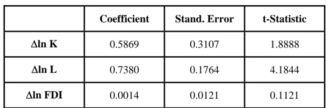
The results, which are in Table 5 below, are similar to the previous results except that the coefficients associated with capital and labour are now in the expected range. The coefficient for Δln FDI is again positive and not statistically significant.
. . . . . . . . . .
Δln Y
it=
β1Δln K
it+ (1-β
1) Δln L
it+
β
3Δln FDI
it+ e
it(13)
Table 5: Restricted OLS Estimation – International Data Set #1
Coefficient Stand. Error t-Statistic
Δln K 0.5869 0.3107 1.8888
Δln L 0.7380 0.1764 4.1844
Δln FDI 0.0014 0.0121 0.1121
Coefficient Stand. Error t-Statistic
Due to concern over endogeneity, a Hausman test is again used to test whether or not the explanatory variables are exogenous in the growth accounting equation. With p-values of 0.4331 and 0.1587, respectively, we do not reject the hypotheses that Δln FDI and Δln K are exogenous. However, with a p-value of 0.0419, it appears that Δln L is not exogenous. In an attempt to address this problem, the Arellano-Bond estimator is used later in this section.
The results for the OLS estimation of Equation 12, which uses the second international data set, are presented in Table 6.
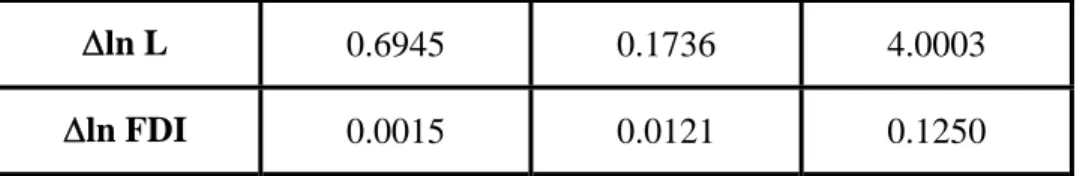
The restriction of constant returns to scale is tested using the unrestricted estimation and with a p-value of 0.1702 we are unable to reject the null hypothesis that the coefficients associated with labour and capital sum to one. Therefore, Equation 15 (below), which imposes the restriction of constant returns to scale, is also estimated and the results are included in Table 6. White standard errors, corrected for the loss of degrees of freedom due to the country specific terms, are in round brackets and t-Statistics are in square brackets.
. . . . . . . . . .
Δln Y
it=
β1Δ(INV/GDP)
it+ (1-β
1) Δln L
it+
β
3Δln FDI
it+ e
it(15)
Table 6: Unrestricted and Restricted
OLS Estimation – International Data Set #2
Δln L 0.6945 0.1736 4.0003
The results are similar to those found using the first set of international data. The coefficients for Δ(INV/GDP) and Δln L are positive and significant and the coefficient for Δln FDI is positive and is not statistically significant.
The Hausman test is again performed for the explanatory variables. The p-values associated with labour, capital and FDI are 0.2626, 0.0000 and 0.6377, respectively. Therefore, it appears that Δln L and Δln FDI are exogenous and that Δ(INV/GDP) is not. As mentioned above, the Arellano-Bond estimator is used later in this section to attempt to address this problem.
Next, the same sequential procedure that was used in Part 1 to determine the optimal number of lags of the growth of FDI stock was performed. It was again
determined that no lags should be included in the regression. The results found above are robust in terms of the number of lags included.
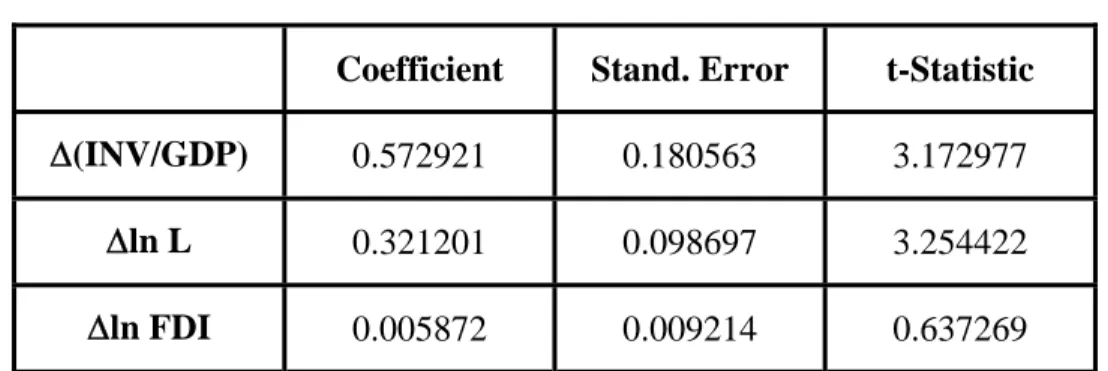
In order to try to address the problem of endogeneity, the Generalized Method of Moments (GMM) estimator developed by Arellano and Bond (1991) is also used and the results are presented in Table 7.
The Sargan test for over-identifying restrictions produces a p-value of 0.1704; therefore, the null hypothesis that there is overall validity of instruments is not rejected.
The coefficients associated with capital and labour are not as expected – both are statistically significant but the coefficient for Δln L is smaller than expected while the coefficient for Δ(INV/GDP) is larger than expected. The coefficient associated with FDI is positive and not statistically significant.
Unrestricted Restricted Δ(INV/GDP) 0.2099 (0.0567) [3.7046] 0.2374 (0.0575) [4.1288] Δln L 0.6425 (0.1063) [6.0440] 0.7626 (0.0575) [13.262] Δln FDI 0.0082 (0.0085) [0.9639] 0.0069 (0.0085) [0.8186]
Table 7: Arellano-Bond – International Data Set #2
The question that was examined in this empirical analysis was: Does FDI bring with it externalities for the host country? Among the results above, it was the OLS
regressions using Canadian data that include between two and five lags of the growth rate of FDI stock that showed that same-period growth in FDI stock has a significantly
positive effect on economic growth. The other coefficients associated with FDI in this study were not statistically significant, although most of them were positive. This analysis was not able to produce a decisive result regarding externalities in the host economy due to increases in the stock of FDI.
Limitations
The empirical tests presented here have several weaknesses and limitations – a few are noted here.
One weakness, which was touched on earlier, is the small size of the data sets – ideally, for the international data sets, there should be a much larger group of countries and a longer time span included.
The models also suffer, undoubtedly, from having important variables omitted. For example, there is not a proxy variable included in the international data sets to represent human capital. I did not include “school enrollment” – a common control variable in growth accounting – because the data was only available every five years for much of the time period studied and since the variable estimated would have been the change in enrollment, I felt that to interpolate for the missing values would have created too much error. A further complication is that an increase in school enrollment would
Coefficient Stand. Error t-Statistic
Δ(INV/GDP) 0.572921 0.180563 3.172977
Δln L 0.321201 0.098697 3.254422
most likely not produce benefits for the economy in question until years after the increase. Creating a more reliable data set was beyond the scope of this paper.
Moreover, this paper looks at the overall economy and does not look at individual sectors. Different areas of the economy could have unique experiences with FDI that would clearly not be captured by a study, such as the one in this paper, that deals with aggregate data.
Section 6: Conclusion
The motivation for this paper came from the debate in recent years over whether FDI is harmful or helpful to the host economy. In Canada, for example, there are many
groups, such as the Chamber of Commerce, that believe Canada should be actively promoting FDI and there are others who think FDI should be more regulated.
The main arguments in favour of promoting FDI are that it will increase the private capital stock of the host economy as well as increase domestic productivity if it is accompanied by positive spillovers.
Some of the arguments in favour of increased restrictions on FDI are the decrease in domestic control of assets and future outflows of profits.
This paper examined one specific aspect of this debate. In the empirical analysis, the question posed was: Does the data suggest that FDI brings with it externalities for the host country?
The framework of the study is a growth accounting empirical model that uses three different data sets. The first is Canadian data and for this set, estimation was carried out using OLS and TSLS. The second and third are assembled using a selection of OECD countries and two different time periods. For these sets, data was pooled and the fixed effects and the Arellano-Bond estimators were used. For all models, growth of GDP was regressed on the growth of FDI stock and on other control variables.
The OLS regressions that used Canadian data and that included between two and five lags of the growth rate of FDI stock showed that same-period growth in FDI stock has a significantly positive effect on economic growth. The other coefficients associated with FDI were not statistically significant – with most being positive and a few being negative. Therefore, this analysis was not able to produce a decisive result regarding externalities in the host economy due to increases in the stock of FDI.
This paper addresses one aspect important to the debate over FDI – the issue of externalities. For future research, a more comprehensive multi-country data set with a longer time span and a more detailed set of explanatory variables may further help to elucidate this issue.
There are also other questions that would be of interest for future research. For example, this paper does not consider the effect of regulations governing FDI on the capital stock of the host economy. It would be interesting to test what happens to the capital stock of the host economy following a change in their regulatory climate. Does the capital stock decrease when tighter restrictions are imposed? If it does, by how much?
Do citizens of the host economy react by investing more in their own country and less abroad, filling or partially filling the vacuum created when the restrictions are imposed on FDI? Or, does the vacuum remain unfilled?
The answers to these questions would help to bring clarity to the overall question of the effect of FDI on host economies and would be complementary to the existing research.
Bibliography
Arellano, M., and S. Bond ,“Some Tests of Specification for Panel Data: Monte Carlo Evidence and an Application to Employment Equations”, Review of Economic Studies Vol. 58, 1991, 277–297.
Blonigen, Bruce A. and Miao Grace Wang, “Inappropriate pooling of wealthy and poor countries in empirical studies”, NBER Working Paper, no. 10378, 2004.
Canadian Chamber of Commerce, “Attracting Foreign Direct Investment to Canada”,
Policy Resolutions Book, 2007, http://www.chamber.ca/article.asp?id=465#intl.
growth?”, University of Minnesota Department of Finance Working Paper, 2002. http://ssrn.com/abstract=314924
Choe, Jong Il, “Do Foreign Direct Investment and Gross Domestic Investment Promote Economic Growth?, Review of Development Economics, vol. 7, 2003, 44-57.
Gellaty, G., D. Sabourin and J. Baldwin, “Changes in Foreign Control under Different Regulatory Climates: Multinationals in Canada”, Statistics Canada: Canadian Economic
Observer, March 2006, 3.10-3.17.
Görg, Holger, David Greenaway, “Much Ado About Nothing? Do Domestic Firms Really Benefit From Foreign Investment?”, Centre for Economic Policy Research Discussion Paper, no. 3485, 2002.
Harrison, Ann, “Openness and Growth: A time-series, cross-country analysis for developing countries”, Journal of Development Economics, vol. 48, 1996, 419- 447.
Henry, Peter Blair, “Capital Account Liberalization: Theory, Evidence, and Speculation”,
Journal of Economic Literature, vol. 45, December 2007, 887-935.
Holden, Michael, “The Foreign Direct Investment Review Process in Canada and Other Countries” Parliamentary Information and Research Service, Economics Division, September 2007
International Monetary Fund (IMF), “Foreign Direct Investment Trends and Statistics", IMF web site, October 2003,
http://www.imf.org/external/np/sta/fdi/eng/2003/102803.htm
Lensink, Robert and Oliver Morrissey, “Foreign Direct Investment: Flows, Volatility, and the Impact on Growth”, Review of International Economics, vol. 14 no.3, 2006, 478-493.
Nehru, V. and A. Dhareshwar, “A new database on physical capital stock: Sources, methodology, and results”, Revista de Analisis Economico, vol. 8 no. 1, 1993, 37- 59.
Statistics Canada, “Canada's International Investment Position (IIP)”, Statistics Canada web site, 2008, n. pag.,
http://www.statcan.ca/cgi-bin/imdb/p2SV.pl?Function=getSurvey&SDDS=1537&lang=en&db=IMDB&dbg=f&ad m=8&dis=2
United Nations Conference on Trade and Development (UNCTD), Press Release, 2003, http://www.un.org/News/Press/docs/2003/tad1949.doc.htm
Wooldridge, Jeffrey M., Introductory Econometrics. A Modern Approach, Thomson South-Western, 2006.
Yang, Benhua, “FDI and growth: a varying relationship across regions and over time”,


![[PDF] Support de cours PDF de COVADIS et la 3D avec images et explications - Cours informatique](data:image/gif;base64,R0lGODlhAQABAIAAAP///wAAACH5BAEAAAAALAAAAAABAAEAAAICRAEAOw==)