Non-stationary Intensity-Duration-Frequency curves integrating information concerning teleconnections and climate change.

Accepted Article

Non-stationary Intensity-Duration-Frequency curves integrating

information concerning teleconnections and climate change

Taha B.M.J. Ouarda

, Latifa A. Yousef

, and Christian Charron

1

Canada Research Chair in Statistical Hydro-Climatology, INRS-ETE, 490 de la Couronne, Québec, QC, G1K 9A9, Canada

2

Masdar Institute of Science and Technology, P.O. Box 54224, Abu Dhabi, UAE

*

Corresponding author: T. B. M. J. Ouarda (taha.ouarda@ete.inrs.ca)

Abstract

Rainfall Intensity-Duration-Frequency (IDF) curves are commonly used for the design of water resources infrastructure. Numerous studies reported non-stationarity in meteorological time series. Neglecting to incorporate non-stationarities in hydrological models may lead to inaccurate results. The present work focuses on the development of a general methodology that copes with non-stationarities that may exist in rainfall, by making the parameters of the IDF relationship dependent on the covariates of time and climate oscillations. In the recent literature, non-stationary models are generally fit on data series of specific durations. In the approach proposed here, a single model with a separate functional relation with the return period and the rainfall duration is instead defined. This model has the advantage of being simpler and extending the effective sample size. Its parameters are

This article has been accepted for publication and undergone full peer review but has not been through the copyediting, typesetting, pagination and proofreading process, which may lead to differences between this version and the Version of Record. Please cite this article as doi: 10.1002/joc.5953

Accepted Article

estimated with the maximum composite likelihood method. Two sites in Ontario, Canada and one site in California, USA, exhibiting non-stationary behaviors are used as case studies to illustrate the proposed method. For these case studies, the time and the climate indices Atlantic Multi-decadal Oscillation (AMO) and Western Hemisphere Warm Pool (WHWP) for the stations in Canada, and the time and the climate indices Southern Oscillation Index (SOI) and Pacific Decadal Oscillation (PDO) for the stations in USA are used as covariates. The Gumbel and the Generalized Extreme Value distributions are used as the time dependent functions in the numerator of the general IDF relationship. Results shows that the non-stationary framework for IDF modeling provides a better fit to the data than its stationary counterpart according to the Akaike Information Criterion. Results indicate also that the proposed generalized approach is more robust than the the common approach especially for stations with short rainfall records (e.g. R2 of 0.98 compared to 0.69 for duration of 30 min and a sample size of 27 years).

Keywords: Non-stationarity; Hydro-meteorological modeling; Rainfall;

Accepted Article

1. Introduction

Rainfall Intensity-Duration-Frequency (IDF) curves are commonly used for planning, designing and operating water resources infrastructure. Their importance in the design of sewer systems, for example, can be attributed to their physical link to the time of concentration, which is defined as the time required for a rainfall drop to flow from the farthest point in the catchment to the point of the sewer system for which the design is made. Runoff reaches a peak at the time of concentration when the entire watershed contributes to the flow at the outlet (Chow et al., 1988). The design intensity duration is then equal to the time of concentration. IDF relationships are generally represented on plots of the intensity vs. the duration, using a family of curves representing specific return periods. The first uses of IDF relationships date back to the 1930’s (Bernard, 1932), while the first construction of geographical maps for IDF relationships in the USA dates back to the early 1960’s (Hershfield, 1961). Today, IDF curves have been developed in most countries (Koutsoyiannis et al., 1998; Willems, 2000; Madsen et al., 2002; Bougadis and Adamowski, 2006; Langousis and Veneziano, 2007; Elsebaie, 2012).

Classical frequency analysis provides adequate engineering design values when the data series from which the probability distribution parameters are to be estimated comes from a stationary distribution and the observations are independent or weakly dependent. In contrast to its classical stationary alternative, a non-stationary data series is one in which the statistics of the sample (mean, variance and covariance) change over time. Non-stationarity in hydrologic records can be attributed to local anthropogenic impacts, such as deforestation and other land use change, or to global climate change and low frequency

Accepted Article

climate oscillations (Milly et al., 2008). Considering that rainfall characteristics are used for the design and management of water resources infrastructures, it is essential to address properly the non-stationarity in rainfall extremes.

The literature indicates that the effects of climate changes on precipitation and runoff have not been given appropriate attention (Semadeni-Davies et al., 2008, Chiew et al., 2009, Arnbjerg-Nielsen, 2012). The stationarity of rainfall records has been studied recently in various parts of the world, with results showing significant trends in the statistical parameters of the analyzed records. Mekis and Hogg (1999) concluded in a study on the Canadian national rainfall time series that an increase in the mean precipitation has occurred over the years 1948–95, with the greatest increase happening in the autumn. Trends in extreme rainfall in Southeast Asia and the South Pacific were examined by Manton et al. (2001), with the results indicating an increase in the proportion of annual rainfall from extreme events, and a decline in the frequency of extreme rainfall events. Westra et al. (2013) analyzed trends in annual maximum daily precipitation on a global scale and detected an increase in trends for the majority of stations.

Non-stationarity in hydro-meteorological variables can also be related to climate oscillation phenomena. Numerous studies have shown that precipitation anomalies can be related to climate indices. Shabbar et al. (1997) provided a detailed analysis of the spatial and temporal behavior in precipitation responses over Canada, and found that they relate to the two extreme phases of the Southern Oscillation (SO). Thiombiano et al. (2017) proposed a non-stationary peaks-over-threshold model to study Southeastern Canada extreme daily precipitation amounts. In this model, the scale parameter of the generalized

Accepted Article

Pareto distribution was allowed to vary as a function of two covariates, the Arctic Oscillation and the Pacific North American climate indices, and the variability was modeled using a B-spline function. Evans et al. (2009) indicated that the observed decline in rainfall over South Australia is linked to increasing Sea Surface Temperatures (SSTs) in the eastern Indian Ocean. Willems (2013b) found that rainfall extremes in Europe have oscillatory behavior at multidecadal time scales, and that the recent upward trend in these extremes for central-western Europe is partly related to a positive phase of this oscillation. An examination of rainfall in Brussels, Belgium, showed that rainfall extremes are temporarily clustered due to the presence of multi-decadal climate oscillations (Willems, 2013a). Ouarda et al. (2014), Chandran et al. (2015), Niranjan Kumar and Ouarda (2014) and Niranjan Kumar et al. (2016) demonstrated the influence of a number of climate oscillation indices on the rainfall regime in parts of the Arabian Peninsula. Ouarda and El-Adlouni (2011) presented a general Bayesian estimation approach for the parameters of hydrological frequency models with covariates. The proposed approach was illustrated in a case study for a station in Southern California, and illustrated the effect of the Southern Oscillation Index (SOI) on annual maximum precipitations.

A number of studies have focused on the development of IDF curves with consideration of non-stationarity (Nguyen et al., 2008; Mirhosseini et al., 2013; Rodríguez et al., 2014; Hassanzadeh et al., 2014; Srivastav et al., 2014; Cheg and AghaKouchak, 2014; Yilmaz et al., 2014; Yilmaz and Perera, 2014; Yousef and Ouarda, 2015; Chandra et al., 2015; Agilan and Umamahesh, 2016; Lima et al., 2016; Ganguli and Coulibaly, 2017; Sarhadi and Soulis, 2017; So et al., 2017; Agilan and Umamahesh, 2018; Ragno et al.,

Accepted Article

2018). In several studies, General Circulation Models (GCMs) and Regional Climate Models (RCMs) are used for assessment of future rainfall events (Nguyen et al., 2008, Mirhosseini et al., 2013, Rodríguez et al., 2014; Hassanzadeh et al., 2014; Srivastav et al., 2014; Chandra et al., 2015; Lima et al., 2016). Nguyen et al. (2008) proposed a statistical downscaling approach, based on the scale invariance concept, to incorporate GCM outputs in the derivation of IDF curves and the estimation of urban design storms for current and future climate scenarios. A regional analysis was then performed to estimate the scaling parameters of extreme rainfall processes for locations with limited or without data. Rodríguez et al. (2014) also applied a statistical downscaling approach to outputs of five GCMs for the simulation of daily and sub-daily rainfall series for a number of stations in Barcelona, Spain, and calculated factors that represent climate change. These climate change factors are defined as the ratio between rainfall intensity in a future climatic scenario and the intensity in the present climate.

IDF models produced using GCM outputs, however, are not “real” non-stationary models; they are simply stationary models that are generated for specified periods of time within a large time frame. A non-stationary model should evolve with the variation of the factors causing the time series to exhibit a trend, or an oscillatory pattern. This non-stationary approach has been applied in several studies for the frequency analysis of hydrological variables. Strupczewski et al. (2001) incorporated hydrological non-stationarity into at-site flood frequency analysis (FFA). A regional non-stationary flood frequency model was proposed by Cunderlik and Burn (2003) that assumes non-stationarity in the first two moments of the time series. El Adlouni et al. (2007) developed a method for

Accepted Article

the estimation of probability distribution parameters involving covariates. Nasri et al. (2013) proposed a Bayesian B-Spline estimator of the parameters and quantiles of the Generalized Extreme Value (GEV) model with covariates.

The formulation of Flood Duration Frequency (QDF) models was derived from IDF models, yet developments in the area of QDF have been happening faster than those in IDF modeling (Javelle et al., 2002, Cunderlik and Ouarda, 2007). A key assumption in traditional QDF modeling is that the model’s parameters are stationary over time, which

has proven to be an incorrect assumption in some cases. New QDF models have been developed with parameters that incorporate dependence on time. Cunderlik et al. (2007) developed a local non-stationary QDF model. Trend analysis was used to identify time-dependent components of the second-order model and predict how they would change in the future. The applied approach assumes non-stationarity in the first two moments of the series. The model was applied to a streamflow data series from British Columbia, Canada, with the results showing that the quantiles estimated by the local non-stationary QDF model were significantly lower than those estimated by the standard QDF technique. Cunderlik and Ouarda (2006) introduced the key concepts of a non-stationary approach to regional QDF modeling. The model was tested and compared to the traditional stationary regional QDF model using a group of homogeneous sites in Quebec, Canada, with the results showing that the quantiles estimated by the traditional stationary QDF approach at the end of the observation period were significantly overestimated.

There was recently a growing interest in non-stationary IDF models for which the parameters are dependent on covariates (Cheg and AghaKouchak, 2014; Yilmaz et al.,

Accepted Article

2014; Yilmaz and Perera, 2014; Yousef and Ouarda, 2015; Agilan and Umamahesh, 2016; Ganguli and Coulibaly, 2017; Sarhadi and Soulis, 2017; So et al., 2017; Agilan and Umamahesh, 2018; Ragno et al., 2018). In the recent studies that focused on non-stationary IDF curves, a different non-stationary GEV model is generally fit to each data series of a specific duration. However, it is often assumed that IDF curves are modeled by a single model which is dependent on both the return period and the duration (Chow et al., 1988; Koutsoyiannis et al., 1998; Muller et al., 2008; Van de Vyver, 2015). Rossi and Villani (1994) and Koutsoyiannis et al. (1998) introduced a general formula for the IDF relationship in which the rainfall intensity is the product of a function of T and a function of d. The main objective of the present study is to extend the general IDF relationship to the non-stationary framework. The main advantages of this approach are that a simpler model is obtained which eases interpretation and application of the model, there are fewer parameters to estimate and the effective sample size increases because of the pooling of data from the different durations (Veneziano et al., 2007). This is an important feature especially for the small sample sizes often encountered with hydro-meteorological variables. The proposed model introduces climate oscillation indices and time as covariates and allows both the position and the scale parameters of the distribution in the IDF relationship to vary as function of the covariates. This model is validated using case studies from Canada and the USA. A comparison of the general approach proposed in this work with the common approach is also presented. This study focuses also on the graphical representation of non-stationary IDF relationships.

Accepted Article

2. Theoretical background

2.1. Classical IDF relationship formulation

The IDF relationship is commonly used to relate rainfall intensity with its duration and annual frequency. To define the IDF relationship, the series of maximum average intensities ( )i d , _j j1,...,n, is obtained for selected durations d k_k, 1,...,m, where n is the

number of years with measurements and m is the number of duration groups. The average intensity is defined by the depth during the time interval divided by the duration d. The frequency of the maximum intensity i(d) is described in terms of return period T, which is the average time interval between rainfall events that exceed the return level ( )i d . _T

Several IDF relationship formulations have been proposed in the literature. In general, for a given return period, they are special cases of the general formula:





where ω, ν, θ and η are non-negative coefficients. A number of specific formulations can be adapted from the general formula of equation 1 and are commonly used in the hydrological literature (Chow et al., 1988): the Talbot equation (with  1 and  1), the Bernard equation (with  1 and  0), the Kimijima equation (with 1) and the Sherman equation (with  1).

Accepted Article

Rossi and Villani (1994) and Koutsoyiannis et al. (1998) proposed a generalized formulation of the IDF relationship, which can be expressed as follows:

 

 

The advantage of using this formulation is that i d has a separate functional dependence _T( )

on the return period T and the duration d. This approach relies on the assumption of self-similar scaling of annual maximum intensities with the averaging duration d. While separable scaling with d and T was originally derived based on empirical evidence, its validity was later substantiated asymptotically in the context of stochastic self-similar (i.e. multifractal) processes; see e.g. Veneziano and Langousis (2005), Veneziano et al. (2006, 2009), Langousis et al. (2009, 2013), and Tyralis and Langousis (2018). The function b(d) is derived from the denominator in equation 1 and is expressed as:

( ) ( )

b d  d . (3)

Koutsoyiannis et al. (1998) demonstrated that  _{in equation 1 can be neglected and thus}

1

  is assumed. Instead of being estimated empirically, the function a(T) is completely

determined from the distribution function of the maximum rainfall intensity I(d). If the probability distribution of I(d) is F_{I d }

 

 

 

T

   ). Consequently,

the expression for a(T) is given by:

 

Accepted Article

2.3. IDF relationship formulation with the EV probability distribution

For the formulation of the general IDF relationship, any distribution that provides a good fit to the intensities can be introduced. Koutsoyiannis et al. (1998) gave a list of candidate distribution functions that can be incorporated with the general IDF relationship: the GEV, Gamma, Log Pearson type III, Lognormal, Exponential, Pareto and the Gumbel distributions. The Gumbel (EV) distribution function, also termed type I distribution of maxima, or Extreme Value type I distribution, is highly suitable for the modeling of maxima and is traditionally the most commonly used distribution to model rainfall (Chow et al., 1988).

Let us assume that the rainfall intensity I(d) for any duration follows a EV distribution, therefore the distribution of Y will be:

 

where μ and σ are respectively the location and scale parameters. By combining equations 4 and 5, the following expression of a(T) is obtained:

 

The general IDF relationship assuming the EV distribution is then presented in the following form:

 

 





Accepted Article

2.4. IDF relationship formulation with the GEV probability distribution

The GEV distribution is increasingly adopted for rainfall modeling. For instance, Adamowski et al. (1996) recommended the use of the GEV for rainfall modeling in Canada and Koutsoyiannis and Baloutsos (2000) found the GEV to be more suitable than the EV to model rainfall in Greece. Consequently, in this study, the GEV is also used in the formulation of the IDF relationship. Note that the EV is a special case of the GEV distribution.

When the rainfall intensity I(d) for any duration is assumed to follow a GEV distribution, the distribution of Y is written as:

 

where μ, σ and κ are respectively the location, scale and shape parameters. By combining equations 4 and 8, the following expression of a(T) is obtained:

 

The general IDF relationship assuming the GEV distribution is then presented in the following form:

 

 





Accepted Article

2.5. Non-stationary general IDF relationship formulation

For the formulation of the non-stationary general IDF relationship, a number of the model parameters are made dependent on covariates. El Adlouni et al. (2007) incorporated non-stationarity into the GEV distribution function, where the location and scale parameters were made dependent on covariates, either linearly or quadratically. In the context of the IDF relationship, a positive trend in the location parameter (and hence in the mean) will lead to a translation of the curve upwards. A positive trend in the scale parameter (and hence in the variance) will increase the distance between the IDF curves.

The formulation of the Non-stationary IDF relationship proposed in the present study assumes the EV or the GEV distributions. It is assumed also that parameters μ and σ

are dependent upon the covariates while all shape parameters, θ and η for both distributions, and κ for the GEV, are constant. This assumption is frequent in non-stationary models where, for instance, the shape parameter of the GEV is often assumed constant and the location and scale parameter depend upon a covariate (Katz et al, 2002; El Adlouni and Ouarda, 2009). This hypothesis will be verified in the present case study. The EV distribution parameters μ and σ in equations 7 and 10 become then the covariate-dependent

parameters _t and _t. The IDF formulations in equations 7 and 10 are then modified in the non-stationary case to become for the EV and GEV respectively:





Accepted Article





The dependence of _t and _t on the covariate(s) can take any form that would lead to the best goodness of fit of the model to the data. The linear and quadratic dependence forms of parameters on covariates are the easiest and the most commonly adopted in the non-stationary literature. Let us denote Y and t Z the first and second time-dependent t

covariates. Distribution parameters _t and _t for non-stationary models with one covariate are allowed to take the following forms:

0 0 1 2 0 1 2 t t t t Y Y Y           _      , (13) 0 0 1 t t Y        _  . (14)

The quadratic relation with t is not considered for the sake of simplicity. Distribution parameters _t and _t for non-stationary models with two covariates are allowed to take the forms: 0 1 2 2 0 1 2 3 2 0 1 2 3 2 2 0 1 2 3 4 t t t t t t t t t t t t t Y Z Y Y Z Y Z Z Y Y Z Z                      _{  }              , (15) 0 t   . (16)

Accepted Article

In the case of non-stationary models with two covariates, distribution parameter t is made constant to obtain simpler models. Indeed, a large number of parameters would need to be fitted when two covariates are considered, and the limited size of the record may become a limiting factor.

For the classical general IDF relationship incorporating the EV distribution, a vector of 4 distribution parameters  ( , , , )    needs to be estimated while a vector of 5 distribution parameters  ( , , , , )     needs to be estimated for the GEV. In the case of the non-stationary general IDF relationship, additional parameters, depending on the selected model, need to be estimated and the vector of parameters to estimate becomes

0 1 0

( , , , ) ( , ,..., ,..., , )

t t t

            and t (    t, t, , , )( ₀, ₁,...,₀,..., , , )  

for the EV and GEV respectively. The number of parameters ranges from 4 to 8 in the case of the EV and from 5 to 9 in the case of the GEV.

2.6. Parameter estimation

Once the adequate formulation of the IDF relationship has been defined, the unknown parameters need to be estimated. The least-squares method presented in Koutsoyiannis et al. (1998) is inadequate in a non-stationary framework because of the violation of the distributional assumption of homogeneity (Coles, 2001). The maximum likelihood and generalized maximum likelihood methods are generally used with non-stationary models (El Adlouni et al., 2007). The maximum likelihood method has the advantage over other methods of adapting to changes in the model structure (Coles, 2001).

Accepted Article

Let us define ( ; , )f i  , the joint probability density of I 





α is a parameter vector that parameterizes the dependence between intensities I d( _k) and

( _k)

I d _ while  parameterizes the marginal structure. The full likelihood is then given by:

1 1 ( ; ) ( ,..., ; , ) n j jm j L i f i i    



where i_jk denotes the jth intensity value for the duration group k. However, the density ( ; , )

f i  is unknown which makes difficult or impractical the estimation of the full likelihood. Indeed, in the case of IDF curves the maximum rainfall intensities over the different durations are dependent which violates the assumption of independence required in the definition of the likelihood. To overcome this difficulty, a simplified likelihood function for IDF curves is obtained by assuming the independence among the intensities over the different durations. This function is often referred to as the independence likelihood (Chandler and Bate, 2007) and is given by:

1 1 ( ; ) ( ; ) n m ind jk j k L  i f i    



where f i( ; ) is the density function of I d . In practice, the log likelihood ( )

( ; ) log ( ; )

ind ind

l  i  L  i is maximized with an optimization procedure to obtain ˆ , the estimator of  . This method was applied to the IDF relationship in Muller et al. (2008) and Van de Vyver (2015). If ( )I d follows a EV or a GEV distribution, the probability function

Accepted Article

( ) ~ EV( ( ), ( ))

I d  d  d , (19)

( ) ~ GEV( ( ), ( ), )

I d  d  d  (20)

where the parameters of the distribution are expressed as:

( ) ( ) d d       , ( )d (d )      . (21)

In the case of the non-stationary IDF relationship, the distribution parameters are expressed as: ( ) ( ) t t d d       , ( ) ( ) t t d d       . (22)

The independence likelihood can be considered as a special case of the composite likelihood. Varin et al. (2011) defined the composite likelihood as an inference function derived by multiplying a collection of component likelihoods. They are used in several applications as surrogates for the ordinary likelihood when it is too cumbersome or impractical to compute the full likelihood (Varin and Vidoni, 2005).

To compare the goodness-of-fit of different models, information criteria such as the Akaike information criterion (AIC) or Bayesian information criterion (BIC) are generally used where smaller values of these criteria indicate better models. In the framework of composite likelihood, these criteria cannot be used because the second Bartlett identity does not hold, i.e. H( ) J( ) where H( ) E {_ _u( ; )} I is the sensitivity matrix or Hessian, J( ) var { ( ; )}_ u I is the variability matrix, and u( ; ) i  _l_ind( , ) i . Analogous criteria are then used having the forms CL-AIC 2l_ind( ; )ˆ i 2dim( ) and

Accepted Article

ˆ

CL-BIC 2l_ind( ; ) i dim( ) log( ) n where dim( ) is the effective number of parameters estimated by tr{J( )H( ) }  1 . The sample estimates of the sensitivity matrix H and variability matrix J were provided by Varin et al. (2011):

1 1 ˆ _ˆ H( ) ( ; ) n j j u i n      





However, given that the second Bartlett identity is valid for each individual likelihood term, computation of the Hessians can be avoided and an alternate sample estimate can be obtained for the sensitivity matrix by (Varin et al., 2011):

T 1 1 1 ˆ _{ˆ ˆ} H( ) ( ; ) ( ; ) n m jk jk j k u i u i n       



3. Study methodology

The procedure starts by testing whether it is appropriate to build a non-stationary IDF model to represent a specific data set. This is achieved by testing historical records of intensity data for non-stationary signals. A statistical trend test can be applied to the individual series corresponding to different durations. The selected method to perform this test is the revised Mann-Kendall test (Yue and Wang, 2004), which is a modified version of the traditional Mann-Kendall test taking into consideration the effects of autocorrelation. If the intensity record tests positive to the hypothesis of existing trend within the specified confidence interval for the majority of durations, a non-stationary IDF model is built.

Accepted Article

The general IDF model has four parameters on which dependence with covariates can be established. It was assumed above that distribution parameters μ and σ depend upon the covariates while parameters θ and η are kept constant. The following method is applied

to test whether this hypothesis holds. Moving windows of the intensity data with sufficient sizes are created at the selected station. The stationary IDF model is fitted to each window where the parameters are estimated with the maximum composite likelihood method. The revised Mann-Kendall test is then applied to the obtained parameter series to detect any trends in the parameters. Parameters for which a trend is detected should be made dependent on the selected covariate in the non-stationary formulation of the IDF model.

Once this is done, a number of options to represent the dependence of the model parameters on the covariates are tested. The tested models, presented in Subsection 2.5, incorporate parameter dependence on covariates in the linear or the quadratic form. The number of parameters to be estimated varies with the complexity of the model. The parameters of the models are estimated using the maximum composite likelihood method presented in Subsection 2.6. The optimization function fmincon in MATLAB (MATLAB Optimization Toolbox, 2016) which solves constrained non-linear multivariable functions where the upper and lower bounds of the parameters are defined, is used to solve the optimization problem of maximizing equation 14. CL-AIC is computed for each tested model and the one providing the best CL-AIC statistic is considered as the optimal model.

Accepted Article

4. Case studies

Two case studies are used to illustrate the method presented in this study. They include two stations from the Province of Ontario, Canada, and one station from the State of California, USA. Canadian precipitation data were obtained from the online Engineering Climate Datasets (ftp://ftp.tor.ec.gc.ca/Pub/Engineering_Climate_Dataset/IDF/). Precipitation data for the USA were obtained from the Precipitation Frequency Data Server (PDFS) (ftp://hdsc.nws.noaa.gov/pub/hdsc/data/sa/), which is part of the National Oceanic and Atmospheric Administration’s (NOAA) National Weather Service. These databases provide annual maximum precipitation time series for various durations.

Two case studies are used to illustrate the method presented in this study. They include two stations from the Province of Ontario, Canada, and one station from the State of California, USA. Canadian precipitation data were obtained from the online Engineering Climate Datasets (ftp://ftp.tor.ec.gc.ca/Pub/Engineering_Climate_Dataset/IDF/). Precipitation data for the USA were obtained from the Hydrometeorological Design Studies Center (ftp://hdsc.nws.noaa.gov/pub/hdsc/data/sa/), which is part of the National Oceanic and Atmospheric Administration’s (NOAA) National Weather Service. These databases provide annual maximum precipitation time series for various durations.

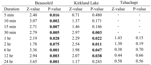
The Canadian database has 9 duration groups from 5 min to 24 hours and the USA database has 6 duration groups from 1 hour to 24 hours. The spatial distribution of the selected stations of the two case studies are presented in Figure 1. The rainfall intensities at the rainfall stations were tested using the revised Mann-Kendall test. The P-value and Z-value results of the Mann-Kendall test are presented in Table 1. Information concerning

Accepted Article

climate indices used in this study is obtained from the NOAA Earth System Research Laboratory (http://www.esrl.noaa.gov/psd/data/climateindices/list/).

The study conducted by Leclerc and Ouarda (2007) for the purpose of regional FFA at ungauged sites presents a number of locations in the Province of Ontario, Canada, which exhibit non-stationary signals. Ontario's climate varies significantly in the different seasons of the year and from one location to another within the Province. The station of Beausoleil (44.85 °N, 79.87 °W) has the particularity of having a significant positive trend for each of

the durations at a significance level of 10%. Given this strong signal, this station is selected in the first case study. Beausoleil is located in Lake Huron’s Georgian Bay in southeastern Ontario. The 27 years of record cover the time period 1977-2007, with a gap from 1993 to 1996.

The maximum annual rainfall depth for the Beausoleil station was tested for correlations with climate oscillations that are known to impact the region (Sutton and Hudson, 2005; Knight et al., 2006; Thiombiano et al., 2017). In this study, the following climate indices were considered: the Atlantic Multi-decadal Oscillation (AMO), the SOI, a measure of El Nino/Southern Oscillation (ENSO), the Pacific Decadal Oscillation (PDO), the Pacific North America (PNA), the Atlantic Oscillation (NAO), the Arctic Oscillation (AO) and the Western Hemisphere Warm Pool (WHWP). Data are available as monthly time series from the National Oceanic and Atmospheric Administration (NOAA) and are updated regularly. These times series are available from 1856 to present for AMO, 1948 to present for PDO and WHWP, 1950 to present for AO, NAO, and PNA, and 1951 to present for SOI. High correlations were found between the intensities for most durations and the

Accepted Article

AMO index as well as the WHWP index. A second station in the Province of Ontario, the Kirkland Lake station (48.15 °N, 80.00 °W), is selected for comparison purposes using the

same climate indices than Beausoleil. This station is located in the eastern part of the Province of Ontario, about 425 km to the north from the Beausoleil station. The 26 years of record cover the time period 1980-2006. Intensity time series at this station show also significant positive trends for most durations at a significance level of 10% and present relationships with the same climate indices.

The second case study deals with a precipitation station from the State of California, USA. A strong significant negative relationship between the annual maximum precipitation in southwestern California and the SOI climate index was demonstrated in El Adlouni et al. (2007). In Nasri et al. (2013), a positive relation between the annual maximal precipitation in southwestern California and the climate index PDO was also identified. El Adlouni et al. (2009) also found a strong relation between SOI and annual maximum precipitation at the Tehachapi station (35.13 °N, -118.45 °W), located in southwestern California. Annual maximum precipitations corresponding to various durations are available for this station in the USA database. The station has a long record of 52 years from 1949 to 2000 and is analyzed in the present study using SOI and PDO as the covariates representing climate oscillations.

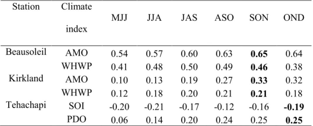
The covariates representing climate indices in this study are climate index averages computed for seasons corresponding to 3 consecutive months (JFM, FMA, MAM, AMJ, MJJ, JJA, JAS, ASO, SON, OND). Correlations between the seasonal climate indices and intensities for different durations are investigated to select the proper season. For prediction

Accepted Article

purposes, seasons corresponding to the covariates are selected before the beginning of the year for which precipitation data are analyzed. Table 2 illustrates the correlations obtained from the season of May-June-July (MJJ) to October-November-December (OND) preceding the observation year for the 1-hour duration precipitation. It shows higher correlations during the season SON for the stations in Canada and during the season OND for the Tehachapi station. This is also true for other durations. Thus, the climate index covariates are defined by the average AMO and WHWP during the season SON for the two Canadian stations, and by the average SOI and PDO during the season OND for the Tehachapi station.

5. Results

Stationary models for EV and GEV were first built considering the models of equations 7 and 10. The stationary IDF curves generated for Beausoleil are presented in Figure 2 for EV. A fourteen-year length moving window, which is approximately half the record length, was then derived and the parameters for the stationary IDF model using EV were estimated for each window. The revised Mann-Kendall test was applied on each parameter series separately. The results indicate that μ and σ exhibit non-stationarity (p-values of the Mann-Kendall test are respectively 0.001 and 0.01), while θ and η do not show any trends (p-values of the Mann-Kendall test are respectively 0.84 and 0.37). This confirms that the correct parameters were selected in Subsection 2.5 to be dependent on the covariates.

Accepted Article

Different non-stationary models are proposed depending on which covariates are included. Models with one covariate include only the “Time” or one of the selected climate

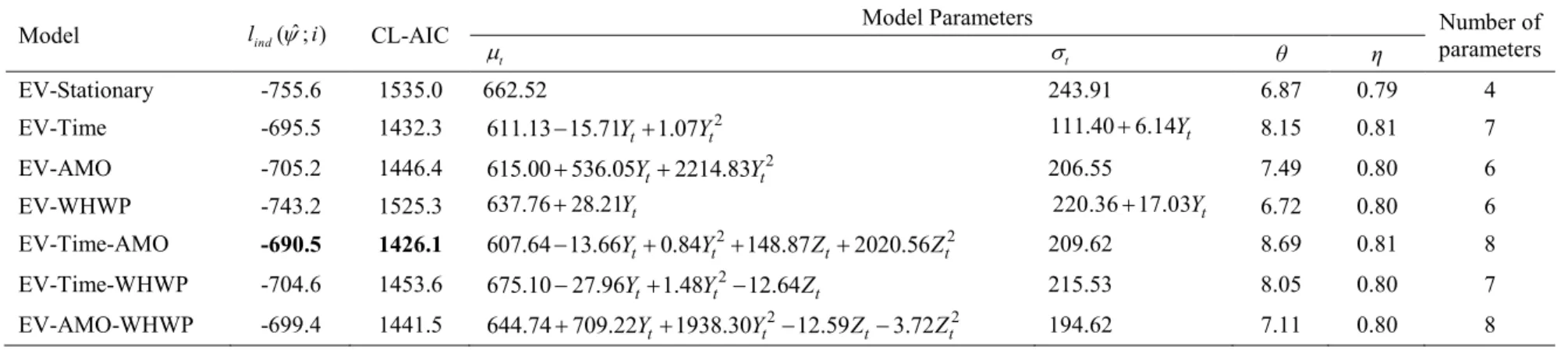
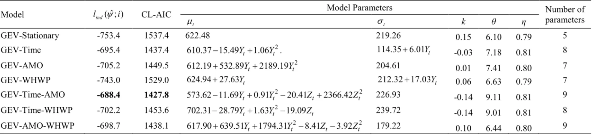
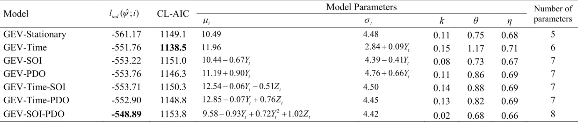
indices separately (AMO, WHWP, SOI and PDO). Models with two covariates include both climate indices (AMO-WHWP or SOI-PDO), or the time and one climate index (Time-AMO, Time-WHWP, Time-SOI and Time-PDO). The distribution parameters are dependent on the covariates according to equations 13-16. Tables 3-8 present the model parameters, log likelihoods and CL-AICs for the stationary and non-stationary IDF models for the EV and GEV distributions at each station. For each model, the optimal parameter relationship with the covariate(s) is determined based on CL-AIC. For all the examples presented in this study, for a given IDF model, the optimal parameter configuration is used. Performances of different IDF models are compared with respect to the complexity-penalizing criterion CL-AIC.

Results show that most non-stationary models lead to improvements, compared to the stationary one, in fitting rainfall intensity data. For instance, at Beausoleil and Kirkland Lake stations, the non-stationary models lead to better fit except for EV-WHWP. It should be noted that using a non-stationary model or the GEV always improves the log likelihood. However, the CL-AIC penalizes models with higher complexity. The GEV with an extra shape parameter, while it always improves the likelihood, it does not provide systematically better goodness-of-fit than the EV with respect to CL-AIC. For instance, in the stationary case, EV is better for Beausoleil and Kirklang, while GEV is better for Tehachapi. Overall, the best models, according to CL-AIC, are EV-Time-AMO for Beausoleil, GEV-Time-AMO for Kirkland Lake, and GEV-Time for Tehachapi. With only one covariate, the best

Accepted Article

models are EV-Time for Beausoleil and Kirkland, and GEV-Time for Tehachapi. With two covariates, the best models are EV-Time-AMO for Beausoleil, GEV-Time-AMO for Kirkland Lake and EV-SOI-PDO for Tehachapi. These results show that non-stationary IDF models, despite their complexity, have a good potential for application in hydrological studies, to integrate information concerning variability and change. It should be noted that better fitting does not necessarily mean more accurate estimates, as IDF fitting within a non-stationary framework allows for an increase in the number of model parameters, with subsequent increase in parameter estimation uncertainty.

Due to the introduction of a fourth variable (the covariate in models with one covariate) in the modeling of the relationship intensity-duration-frequency, the corresponding IDF curves must be represented graphically in a new manner. One suggested representation is to generate a 3D graph where each return period is represented by a surface. Examples of 3D graphs are represented in Figure 3 for Beausoleil, Kirkland Lake and Tehachapi stations for models EV-Time, EV-Time and GEV-Time, which are the best models with 1 covariate. For these graphs, the axes representing the time are extrapolated for 20 years after the last year of observed data, to make them useful for design purposes. Two other suggested representations are possible in 2D. In the first representation, sets of curves are generated, where each set corresponds to a fixed duration. Each curve in a set would then represent a return period. The second representation is, in a certain sense, the opposite of the first where each set would correspond to a fixed return period, and each curve within a set would represent a duration. For illustration purposes, the 2D non-stationary IDF curves for model EV-Time at Kirkland Lake and GEV-Time at Tehachapi

Accepted Article

are presented in Figure 4, for the case corresponding to a fixed duration of 5 minutes and for the case corresponding to a fixed return period of 100 years respectively. For these graphs, the time axis is extrapolated for 20 years after the last year of observed data.

As in the case of non-stationary IDF models incorporating one covariate, for models including 2 covariates, it is necessary to find a new way to represent the IDF relationships. In this case, five variables need to be modeled (intensity, duration, frequency and the two covariates). In this case, it is impossible to represent one model in one figure as in Figure 3. Similar to the non-stationary model with one covariate, there are two methods of representation. In the first, the duration is fixed and a set of surfaces are generated for each return period, and in the second, the return period is fixed and a set of surfaces are generated for each duration. Examples of each representation are shown in Figure 5. In Figures 5a-b, the model EV-SOI-PDO at the Tehachapi station is represented, for a fixed duration of 1 hour and for a fixed return period of 100 years. In Figures 5c-d, the model EV-Time-AMO at the Beausoleil station is represented for a fixed duration of 5 minutes and for a fixed return period of 100 years respectively. Again, the axes of time are extrapolated for 20 years beyond the observation period. It can be noticed in Figure 4 and Figures 5c-d, that the intensity increases after the end of the observed data series in 2007 (during the period of extrapolation). This is due to the quadratic relation of time with the location parameter. Models with time as covariate should be used with extreme care as the direct extrapolation of the currently observed trends can be misleading and may in some cases lead to erroneous results (Ouarda and El Adlouni, 2011).

Accepted Article

Non-stationary models are more complex and require extra work. One question of interest is how do the results of the non-stationary case differ from the simpler stationary case? To answer this question, quantiles are computed for two years representing extreme cases and are compared with the stationary case. Examples illustrated here are for the three stations using in each case the model giving the overall best fits (EV-Time-AMO for Beausoleil, GEV-Time-AMO for Kirkland Lake and GEV-Time for Tehachapi). For the models including Time and AMO as covariates, two years with extreme observed values of AMO corresponding to opposite phases are selected. The aim is to compare the quantiles when the climate index goes from one extreme to another. The selected years are 1983 and 2004, where the values of -0.34 and 0.40 are observed respectively. For the model GEV-Time at Tehachapi, the quantiles are computed for the first and last years of the recorded series with the aim of illustrating the temporal evolution of the quantiles. Figure 6 illustrates the obtained quantiles for T=10 and T=100 years, and for both the stationary and the non-stationary cases. It can be observed that predicted quantiles vary considerably for the two years illustrated with the non-stationary IDF model. For instance, the difference between the 10-year quantiles for these two years represent on average 33%, 31% and 41% of the stationary 10-year quantile respectively for the Beausoleil, Kirkland Lake and Tehachapi stations.

Parsimony issues are important in hydrological sciences due to the generally short length of hydrological records. The case of the stations in Canada, with only 27 and 26 years of record, illustrates commonly encountered record lengths in hydrological applications. It is clear that the use of a model incorporating more than one covariate would

Accepted Article

not be advisable in practice for the case study discussed in the present work. However, the results corresponding to a number of complex models were also presented, with the objective of illustrating how non-stationary IDF curves can be used in practice. This application was treated more like an academic case study that is used to illustrate a new approach. In practice, extreme care needs to be taken when selecting the level of complexity of the model when building non-stationary IDF curves. The dynamics of precipitation in the region of study (generating phenomena, teleconnections, regional signals, etc.) need also to be studied and will be helpful in identifying the appropriate model to use and the number of covariates to incorporate in the models. If a long record is available (70 years of data, for instance), models incorporating more than one covariate may be tested and their results can be used by decision makers to compare a number of scenarios. There is a clear trade-off between adopting simple models with a small number of parameters, and not ignoring any significant signals of non-stationarity (trends or teleconnection induced variability).

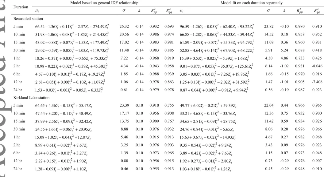
As noted in the introduction, an approach frequently adopted in non-stationary IDF modeling is to define separate non-stationary models for the different durations. This approach is compared here to the general approach proposed in this study. For that aim, the parameters _t and _t of the generalized model are scaled for the different durations using equations 22. This way, distribution parameters _t( )d and _t( )d are derived for each duration while parameter k is constant. Then, separate non-stationary models are fit to the maximum intensities of the different durations using the same distribution and same forms than the general model. This method is applied to the cases of the GEV model with Time

Accepted Article

and climate index giving the best fits for each station: GEV-Time-AMO for Beasoleil and Kirkland Lake, and GEV-Time-PDO for Tehachapi. The parameters obtained with both approaches are presented in Table 9. The coefficient of determination 2

PP

R associated with

the probability plot and the coefficient of determination 2

QQ

R associated with the quantile

plot are used as goodness-of-fit measures.

The results in Table 9 show that, for stations Beausoleil and Kirkland Lake, which have short records of 27 years and 26 years respectively, the general IDF model is often better than the separate IDF models. There are durations for Beausoleil for which the individual models provide poor estimates (e.g. for 30 min, 1 hr, 2 hr and 12 hr). In the case of Beausoleil, the sample size may be too small to estimate the parameters considering that the models used are also fairly complex with 7 parameters. For the Tehachapi station with a longer data record of 52 years, the parameters and performances of both approaches are similar. It can be concluded that for long data records, there is no significant difference between the generalized model and separate models. However, for short data records, the generalized approach is more robust.

6. Conclusions and recommendations

A general methodology for modeling IDF relationships in a non-stationary framework is presented and tested using rainfall intensity data from two stations in the Province of Ontario in Canada and one station in the southwest part of the State of California, USA. The location and scale parameters of the IDF relationship were modeled

Accepted Article

as dependent on time and climate indices for the tested stations. The approach proposed here differs from the recent works published on non-stationary IDF curves in that a single nonstationary model is fit on the intensities of all durations instead of fitting non-stationary models for each specific duration. The main advantage of the proposed approach is that the effective sample size is considerably larger with the use of the aggregated data while the number of parameters to estimate is minimal. This feature is especially important for small sample sizes often encountered with hydro-meteorological variables. Model parameters were estimated by the optimization of the independence likelihood, a special case of composite likelihood in which the independence of the maximum intensities for the different durations is assumed. Selection of optimal models was made with an information criterion analogous to AIC and adapted for the case of composite likelihood.

Non-stationary modeling with covariates of time and climate oscillations was shown in this study to lead to a better fit to the data of the tested station. Neglecting these variables would produce IDF models that are less accurate when the rainfall in a particular area exhibits a strong dependence on time, climate indices, or both. The findings of this study show that it is important to review and update IDF relationships in order to design and manage water structures with consideration of climate variability and change. Stationary IDF models are still of high value and should not be neglected. It is only through a thorough evaluation of the results corresponding to all scenarios that appropriate design and management decisions can be taken.

Future work should focus on testing the developed methodology in other regions where a strong non-stationarity is observed in rainfall records, in order to evaluate the true

Accepted Article

benefits from using non-stationary models. The procedure developed by El Adlouni and Ouarda (2009), which is based on the Birth-Death (BD) Markov Chain Monte Carlo (MCMC) algorithm for the joint estimation of the parameters of non-stationary models and identification of the most appropriate model, could be adapted to IDF models. This may facilitate the adoption of these models in practice.

Acknowledgments

Rainfall annual maximum data for the stations in Canada were obtained from the Engineering Climate Datasets of Environment and Climate Change Canada at ftp://ftp.tor.ec.gc.ca/Pub/Engineering_Climate_Dataset/IDF/. Rainfall annual maximum data for the station in the USA were obtained from the Hydrometeorological Design Studies Center of the NOAA’s National Weather Service at

ftp://hdsc.nws.noaa.gov/pub/hdsc/data/sa/. Climate indices were obtained from the

NOAA’s Earth System Research Laboratory at

http://www.esrl.noaa.gov/psd/data/climateindices/list/. The authors are grateful to the Editor, Dr. Radan Huth, to the Associate Editor, Dr. Sergey K. Gulev, and to three anonymous reviewers for their comments which helped improve the quality of the manuscript.

Accepted Article

References

Adamowski, K., Alila, Y., & Pilon, P.J. (1996). Regional rainfall distribution for Canada. Atmospheric Research, 42(1-4), 75-88. doi:10.1016/0169-8095(95)00054-2.

Agilan, V., & Umamahesh, N. V. (2016). Modelling nonlinear trend for developing non‐

stationary rainfall intensity–duration–frequency curve. International Journal of Climatology, 37(3), 1265-1281. doi:10.1002/joc.4774

Agilan, V., & Umamahesh, N. V. (2018). Covariate and parameter uncertainty in non‐

stationary rainfall IDF curve. International Journal of Climatology, 38(1), 365-383. doi:10.1002/joc.5181

Arnbjerg-Nielsen, K. (2012). Quantification of climate change effects on extreme precipitation used for high resolution hydrologic design. Urban Water Journal, 9(2), 57-65. doi:10.1080/1573062x.2011.630091

Bernard, M. M. (1932). Formulas for rainfall intensities of long duration. Transactions of the American Society of Civil Engineers, 96, 592-606.

Bougadis, J., & Adamowski, K. (2006). Scaling model of a rainfall intensity-duration-frequency relationship. Hydrological Processes, 20(17), 3747-3757. doi:10.1002/hyp.6386

Chandler, R. E., & Bate, S. (2007). Inference for clustered data using the independence loglikelihood. Biometrika, 94(1), 167-183. doi:10.1093/biomet/asm015

Accepted Article

Chandra, R., Saha, U., & Mujumdar, P. P. (2015). Model and parameter uncertainty in IDF relationships under climate change. Advances in Water Resources, 79, 127-139. doi:https://doi.org/10.1016/j.advwatres.2015.02.011

Chandran, A., Basha, G., & Ouarda, T. B. M. J. (2016). Influence of climate oscillations on temperature and precipitation over the United Arab Emirates. International Journal of Climatology, 36(1), 225-235. doi:10.1002/joc.4339

Cheng, L., & AghaKouchak, A. (2014). Nonstationary Precipitation Intensity-Duration-Frequency Curves for Infrastructure Design in a Changing Climate. Scientific Reports, 4, 7093. doi:10.1038/srep07093

Cheng, L., AghaKouchak, A., Gilleland, E., & Katz, R. W. (2014). Non-stationary extreme value analysis in a changing climate. Climatic Change, 127(2), 353-369. doi:10.1007/s10584-014-1254-5

Chiew, F. H. S., Teng, J., Vaze, J., Post, D. A., Perraud, J. M., Kirono, D. G. C., & Viney, N. R. (2009). Estimating climate change impact on runoff across southeast Australia: Method, results, and implications of the modeling method. Water Resources Research, 45(10). doi:10.1029/2008wr007338

Chow, V. T., Maidment, D. R., & Mays, L. W. (1988). Applied hydrology. New York: McGraw-Hill.

Coles, S. (2001). An introduction to statistical modeling of extreme values. London: Springer.

Accepted Article

Cunderlik, J. M., & Burn, D. H. (2003). Non-stationary pooled flood frequency analysis. Journal of Hydrology, 276(1–4), 210-223. doi:10.1016/S0022-1694(03)00062-3

Cunderlik, J. M., Jourdain, V., Quarda, T. B. M. J., & Bobée, B. (2007). Local Non-Stationary Flood-Duration-Frequency Modelling. Canadian Water Resources Journal / Revue canadienne des ressources hydriques, 32(1), 43-58. doi:10.4296/cwrj3201043

Cunderlik, J. M., & Ouarda, T. B. M. J. (2006). Regional flood-duration-frequency modeling in the changing environment. Journal of Hydrology, 318(1-4), 276-291. doi:10.1016/j.jhydrol.2005.06.020

Cunderlik, J. M., & Ouarda, T. B. M. J. (2007). Regional flood-rainfall duration-frequency modeling at small ungaged sites. Journal of Hydrology, 345(1-2), 61-69. doi:10.1016/j.jhydrol.2007.07.011

El Adlouni, S., Ouarda, T. B. J. M., Zhang, X., Roy, R., & Bobee, B. (2007). Generalized maximum likelihood estimators for the nonstationary generalized extreme value model. Water Resources Research, 43(3), W03410. doi:10.1029/2005WR004545

El Adlouni, S., & Ouarda, T. B. M. J. (2008). Comparison of methods for estimating the parameters of the non-stationary GEV model. Revue des sciences de l'eau, 21(1), 35-50. doi:10.7202/017929ar

El Adlouni, S., & Ouarda, T. B. M. J. (2009). Joint Bayesian model selection and parameter estimation of the generalized extreme value model with covariates using birth-death

Accepted Article

Markov chain Monte Carlo. Water Resources Research, 45(6), W06403. doi:10.1029/2007wr006427

Elsebaie, I. H. (2012). Developing rainfall intensity–duration–frequency relationship for two regions in Saudi Arabia. Journal of King Saud University-Engineering Sciences, 24(2), 131-140.

Evans, A. D., Bennett, J. M., & Ewenz, C. M. (2009). South Australian rainfall variability and climate extremes. Climate Dynamics, 33(4), 477-493. doi:10.1007/s00382-008-0461-z

Ganguli, P., & Coulibaly, P. (2017). Does nonstationarity in rainfall require nonstationary intensity–duration–frequency curves? Hydrology and Earth System Sciences, 21(12), 6461-6483. doi:10.5194/hess-21-6461-2017

Gringorten, I. I. (1963). A plotting rule for extreme probability paper. Journal of Geophysical Research, 68(3), 813-814. doi:10.1029/JZ068i003p00813

Hassanzadeh, E., Nazemi, A., & Elshorbagy, A. (2014). Quantile-Based Downscaling of Precipitation Using Genetic Programming: Application to IDF Curves in Saskatoon. Journal of Hydrologic Engineering, 19(5), 943-955. doi:10.1061/(asce)he.1943-5584.0000854

Hershfield, D. M. (1961). Rainfall frequency atlas of the United States: For durations from 30 minutes to 24 hours and return periods from 1 to 100 years. Washington, DC: Department of Commerce. Weather Bureau.

Accepted Article

Javelle, P., Ouarda, T. B. M. J., Lang, M., Bobée, B., Galéa, G., & Grésillon, J.-M. (2002). Development of regional flood-duration–frequency curves based on the index-flood method. Journal of Hydrology, 258(1–4), 249-259. doi:10.1016/S0022-1694(01)00577-7

Katz, R. W., Parlange, M. B., & Naveau, P. (2002). Statistics of extremes in hydrology. Advances in Water Resources, 25(8–12), 1287-1304. doi:10.1016/S0309-1708(02)00056-8

Knight, J.R., Folland, C.K. & Scaife, A.A. (2006). Climate impacts of the Atlantic Multidecadal Oscillation. Geophysical Research Letters, 33(17). doi:10.1029/2006GL026242.

Koutsoyiannis, D. & Baloutsos, G. (2000). Analysis of a long record of annual maximum rainfall in Athens, Greece, and design rainfall inferences. Natural Hazards, 22(1), 29-48. doi:10.1023/a:1008001312219.

Koutsoyiannis, D., Kozonis, D., & Manetas, A. (1998). A mathematical framework for studying rainfall intensity-duration-frequency relationships. Journal of Hydrology, 206(1–2), 118-135. doi:10.1016/S0022-1694(98)00097-3

Langousis, A., Carsteanu, A. A., & Deidda, R. (2013). A simple approximation to multifractal rainfall maxima using a generalized extreme value distribution model. Stochastic Environmental Research and Risk Assessment, 27(6), 1525-1531. doi:10.1007/s00477-013-0687-0

Accepted Article

Langousis, A., & Veneziano, D. (2007). Intensity-duration-frequency curves from scaling representations of rainfall. Water Resources Research, 43(2). doi:10.1029/2006WR005245

Langousis, A., Veneziano, D., Furcolo, P., & Lepore, C. (2009). Multifractal rainfall extremes: Theoretical analysis and practical estimation. Chaos, Solitons & Fractals, 39(3), 1182-1194. doi:doi.org/10.1016/j.chaos.2007.06.004

Leclerc, M., & Ouarda, T. B. J. M. (2007). Non-stationary regional flood frequency analysis at ungauged sites. Journal of Hydrology, 343(3-4), 254-265. doi:10.1016/j.jhydrol.2007.06.021

Lima, C. H. R., Kwon, H.-H., & Kim, J.-Y. (2016). A Bayesian beta distribution model for estimating rainfall IDF curves in a changing climate. Journal of Hydrology, 540, 744-756. doi:10.1016/j.jhydrol.2016.06.062

Madsen, H., Mikkelsen, P. S., Rosbjerg, D., & Harremoës, P. (2002). Regional estimation of rainfall intensity-duration-frequency curves using generalized least squares regression of partial duration series statistics. Water Resources Research, 38(11), 21-21-21-11. doi:10.1029/2001wr001125

Manton, M. J., Della-Marta, P. M., Haylock, M. R., Hennessy, K. J., Nicholls, N., Chambers, L. E., . . . Yee, D. (2001). Trends in extreme daily rainfall and temperature in Southeast Asia and the South Pacific: 1961–1998. International Journal of Climatology, 21(3), 269-284. doi:10.1002/joc.610

Accepted Article

Mekis, E., & Hogg, W. D. (1999). Rehabilitation and analysis of Canadian daily precipitation time series. Atmosphere-Ocean, 37(1), 53-85. doi:10.1080/07055900.1999.9649621

Milly, P. C. D., Betancourt, J., Falkenmark, M., Hirsch, R. M., Kundzewicz, Z. W., Lettenmaier, D. P., & Stouffer, R. J. (2008). Stationarity Is Dead: Whither Water Management? Science, 319(5863), 573-574. doi:10.1126/science.1151915

Mirhosseini, G., Srivastava, P., & Stefanova, L. (2013). The impact of climate change on rainfall Intensity–Duration–Frequency (IDF) curves in Alabama. Regional Environmental Change, 13(S1), 25-33. doi:10.1007/s10113-012-0375-5

Muller, A., Bacro, J.-N., & Lang, M. (2008). Bayesian comparison of different rainfall depth–duration–frequency relationships. Stochastic Environmental Research and Risk Assessment, 22(1), 33-46. doi:10.1007/s00477-006-0095-9

Nguyen, V. T. V., Desramaut, N., & Nguyen, T. D. (2008). Estimation of urban design storms in consideration of GCM-based climate change scenarios. In Water and Urban Development Paradigms (pp. 347-356): CRC Press.

Niranjan Kumar, K., & Ouarda, T. B. M. J. (2014). Precipitation variability over UAE and global SST teleconnections. Journal of Geophysical Research: Atmospheres, 119(17), 10,313-310,322. doi:10.1002/2014JD021724

Niranjan Kumar, K., Ouarda, T. B. M. J., Sandeep, S., & Ajayamohan, R. S. (2016). Wintertime precipitation variability over the Arabian Peninsula and its relationship

Accepted Article

with ENSO in the CAM4 simulations. Climate Dynamics, 47(7-8), 2443-2454. doi:10.1007/s00382-016-2973-2

Ouarda, T. B. M. J., Charron, C., Niranjan Kumar, K., Marpu, P. R., Ghedira, H., Molini, A., & Khayal, I. (2014). Evolution of the rainfall regime in the United Arab

Emirates. Journal of Hydrology, 514(0), 258-270.

doi:10.1016/j.jhydrol.2014.04.032

Ouarda, T. B. M. J., & El-Adlouni, S. (2011). Bayesian Nonstationary Frequency Analysis of Hydrological Variables. JAWRA Journal of the American Water Resources Association, 47(3), 496-505. doi:10.1111/j.1752-1688.2011.00544.x

Ragno, E., AghaKouchak, A., Love Charlotte, A., Cheng, L., Vahedifard, F., & Lima Carlos, H. R. (2018). Quantifying Changes in Future Intensity‐Duration‐Frequency

Curves Using Multimodel Ensemble Simulations. Water Resources Research, 54(3), 1751-1764. doi:10.1002/2017WR021975

Rodríguez, R., Navarro, X., Casas, M. C., Ribalaygua, J., Russo, B., Pouget, L., & Redaño, A. (2014). Influence of climate change on IDF curves for the metropolitan area of Barcelona (Spain). International Journal of Climatology, 34(3), 643-654. doi:10.1002/joc.3712

Rossi, F., & Villani, P. (1994). A project for regional analysis of floods in Italy. In G. Rossi, N. Harmancioğlu, & V. Yevjevich (Eds.), Coping with Floods (pp. 193-217). Dordrecht: Springer Netherlands.

Accepted Article

Sarhadi, A., & Soulis Eric, D. (2017). Time‐varying extreme rainfall intensity‐duration‐

frequency curves in a changing climate. Geophysical Research Letters, 44(5), 2454-2463. doi:10.1002/2016GL072201

Semadeni-Davies, A., Hernebring, C., Svensson, G., & Gustafsson, L.-G. (2008). The impacts of climate change and urbanisation on drainage in Helsingborg, Sweden: Combined sewer system. Journal of Hydrology, 350(1–2), 100-113. doi:10.1016/j.jhydrol.2007.05.028

Shabbar, A., Bonsal, B., & Khandekar, M. (1997). Canadian Precipitation Patterns Associated with the Southern Oscillation. Journal of Climate, 10(12), 3016-3027. doi:10.1175/1520-0442(1997)010<3016:cppawt>2.0.co;2

Sherif, M., Akram, S., & Shetty, A. (2009). Rainfall Analysis for the Northern Wadis of United Arab Emirates: A Case Study. Journal of Hydrologic Engineering, 14(6), 535-544. doi:10.1061/(asce)he.1943-5584.0000015

So, B.-J., Kim, J.-Y., Kwon, H.-H., & Lima, C. H. R. (2017). Stochastic extreme downscaling model for an assessment of changes in rainfall intensity-duration-frequency curves over South Korea using multiple regional climate models. Journal of Hydrology, 553, 321-337. doi:10.1016/j.jhydrol.2017.07.061

Srivastav, R. K., Schardong, A., & Simonovic, S. P. (2014). Equidistance Quantile Matching Method for Updating IDFCurves under Climate Change. Water Resources Management, 28(9), 2539-2562. doi:10.1007/s11269-014-0626-y