THÈSE
THÈSE
En vue de l’obtention du
DOCTORAT DE L’UNIVERSITÉ DE TOULOUSE
Délivré par : l’Université Toulouse 3 Paul Sabatier (UT3 Paul Sabatier)
Présentée et soutenue le 31/05/2019 par : Phuong Lan VU
Spatial Altimetry, GNSS Reflectometry and Marine Surcotes Altimétrie Spatiale, Réflectométrie GNSS et Surcotes Marines
JURY
Guy WÖPPELMANN Université de La Rochelle Rapporteur
Aldo SOTTOLICHIO Université de Bordeaux Rapporteur
Benoit LAIGNEL Université de Rouen Examinateur
Guillaume RAMILLIEN
Université Paul Sabatier Examinateur
Anny CAZENAVE LEGOS, OMP Examinateur
Dongkai YANG Beihang University, Beijing Shi, Chine
Examinateur José DARROZES Université Paul Sabatier Directeur de thèse Frédéric FRAPPART Université Paul Sabatier Co-directeur de thèse
Minh Cuong HA IDAT, Vietnam Invité
École doctorale et spécialité :
SDU2E : Sciences de la Terre et des Planètes Solides Unité de Recherche :
Géoscience Environnement Toulouse(UMR 5563) Directeur(s) de Thèse :
José DARROZES et Frédéric FRAPPART Rapporteurs :
vatrice, s’appuyant sur des plateformes existantes, de suivi des principaux facteurs influençant la dynamique côtière. Lors de mon étude j’ai développé des suivis basés sur un outil classique: l’altimétrie satellitaire. Mon approche s’est appuie sur les nou-velles missions spatiales dont j’ai évalué l’apport sur la zone côtière qui est la plus critique qui est la plus critique du point de vue socio-économique. J’ai plus spécifique-ment regardé la façade atlantique entre La Rochelle et Bayonne. Je me suis ensuite intéressée à une technique originale basée sur la réflexion des ondes GNSS (GNSS-R). Ces outils nous permettent de surveiller précisément les diverses ondes de marée et de détecter des phénomènes plus singuliers comme la tempête Xynthia (2010) qui a affectée le Sud de l’Europe. Ces outils démontrent qu’il est possible aussi de suivre la dynamique côtière liée aux variations de houle et son impact sur l’érosion côtière, et même les effets de la forte dépression atmosphérique associée à Xynthia et qui a eu un impact visible sur le niveau local de l’océan atlantique. Ma thèse repose sur deux approches complémentaires basées sur deux échelles d’analyse, l’une globale as-sociée à l’altimétrie satellitaire l’autre plus locale, dédiée à la détection des évènements extrêmes et basée sur le réflectométrie.
La première étude s’appuie sur différentes missions altimétriques et nous a permis de suivre les variations du niveau de la mer de la côte atlantique française au Sud du golfe de Gascogne durant la période de 1995-2015. Les données SARAL, dont l’empreinte au sol au de l’ordre de 6 km, montrent qu’il est maintenant possible de s’approcher de la bande côtière jusqu’à ∼10 km avec une grande précision (∼20 cm). La seconde application repose sur le GNSS-R que nous avons utilisé pour suivre la partie protégée de la baie de Saint Jean de Luz. Là encore les résultats sont exceptionnels puisqu’ils nous ont permis de suivre l’impact de la tempête Xynthia. J’ai ainsi mis en évidence qu’il était possible avec un seul instrument de suivre les effets des marées, et les effets des surcotes marines qui associées à l’impact de la pression atmosphérique donnent une bonne corrélation (R=0.77 entre la composante RC3 et les surcôtes, et R=0.73 avec la pression atmosphérique) durant la tempête. Enfin nous avons aussi regardé ce qui se passe lors de la transition eaux continentales/océaniques pour les deltas du Fleuve Rouge et du Mékong (Vietnam). Et mêmes si les séries temporelles sont assez courtes, les résultats sont plus qu’encourageant puisqu’ils nous ont permis de de suivre les épisodes de crues associées à deux tempêtes tropicales (Mirinae et Nida) et de mesurer le retard entre les chutes de pluies et la propagation de l’onde crue qui montre dans le cas présent un délai de de 48h pour Nida.
Grâce au déploiement dans de nombreux pays de réseaux GNSS permanents, cette technique peut être appliquée lorsqu’une station GNSS permanente est située près du rivage. L’approche GNSS-R peut être alors utilisée pour le suivi des variations du niveau de la mer mais aussi l’impact d’évènements extrêmes. Pour cela nous avons utilisé 3 mois d’enregistrements (janvier-mars 2010) de la station GNSS de Socoa, pour déterminer les composantes, court terme, de la marée dans les signaux GNSS-R et pour identifier la tempête Xynthia. Cette étude est le premier exemple de l’utilisation du GNSS-R pour détecter les surcôtes, les tempêtes par des techniques de décomposition du signal sous forme d’analyse spectrale singulière (SSA) et de transformation en ondelettes continues. L’un des modes de décomposition du SSA était lié aux variations temporelles de surcotes et des fluctuations atmosphériques à travers le baromètre inversé.
Mes travaux montrent que l’altimétrie satellitaire et GNSS-R constituent une alterna-tive très intéressante aux techniques classiques de mesure in situ surtout pour les zones côtières et estuariennes et la surveillance de l’élévation globale du niveau de la mer. Les techniques basées sur l’altimétrie spatiale montrent leur efficacité pour le suivi des niveaux marins en haute mer mais les nouvelles missions montrent qu’il est possible de s’approcher de plus en plus des côtes tout en conservant une très bonne qualité de mesure. Le GNSS-R présente, quant à lui, l’avantage de s’appuyer sur des réseaux nationaux/internationaux et d’avoir de longues chroniques temporelles (>10 ans). Autre point fondamental il peut suivre la dynamique côtière et des deltas.
Mots clés: Hauteur de la surface de la mer; GNSS-R; SNR; altimétrie côtière; maré-graphe; validation; analyse spectrale singulière; transformation en ondelettes continues; baromètre inversé; onde de tempête.
methodology, based on existing platforms, to monitor the main factors influencing coastal dynamics. We propose monitoring based on a classic tool i.e. satellite altimetry but with a focus on new space missions (SARAL, Sentinel-3). Whose contributions will be evaluated, particularly in the coastal zone, which is the most critical from a socio-economic point of view. I have focused my attention on the French Atlantic coast between La Rochelle and Bayonne. We will also rely on an original technique based on the reflection of GNSS positioning satellites (technical known as GNSS-R). These tools will allow us to precisely monitor the various tidal waves, but they have also allowed us to detect more unusual phenomena such as the extreme event of 2010: the storm Xynthia that affected the coasts of southern Europe.These tools demonstrate that it is also possible will also be able to seeto monitor the coastal dynamics related to swell variations and its impact on coastal erosion, and even the effects of the strong atmospheric depression associated with Xynthia, which has had a measurable impact on the local sea level of the Atlantic Ocean. My thesis is focused on two complemen-tary approaches based on two scales of study: the first one is global and used satellite altimetry, the second one is more local and focused on the extreme event detection and it is based on the GNSS reflectometry.
The first study, which I carried out, relies on different satellite altimetry missions (ERS-2, Jason- 1/2/3, ENVISAT, SARAL) which allowed us to follow the sea level vari-ations (SSH) from the French Atlantic coast to the south of the Bay of Biscay during the 1995-2015 period. SARAL data, including a footprint of around 6 km, show that it is now possible to approach the coastal fringe up to ∼ 10 km with a great precision (RMSE ∼ 20 cm). The second application is based on the GNSS-R methodology that we used to track SSH in the inner part of the bay of Saint Jean de Luz – Socoa during the storm Xynthia. Here again the results are exceptional since they allowed us to follow the impact of the storm Xynthia on the local level of the ocean. I thus highlighted that it was possible with only one instrument to follow the effects of the tides, and even the effects of the marine surges which associated to the impact of the atmospheric pressure on the sea level give a good correlation (R = 0.77 between the RC3 component and the surge, and R = 0.73 with the atmospheric pressure) during storm. Finally we also looked at what is happening in the transition between continental and oceanic waters for the deltas of the Red River and Mekong in Vietnam. And, even if the time series are rather short or truncated (Red River) the results are more than encouraging since they allowed us to follow the flooding events associated with two tropical storms (Mirinae and Nida)
and to measure the delay between the rain falls and the propagation of the flood wave which shows in this case a delay of 48 h for Nida.
With the deployment of permanent GNSS networks in many countries, this technique can be applied when a permanent GNSS station is located near the shore. The GNSS-R approach can be used to monitor sea level variations but also the effect of extreme events. For that we used 3 months of recordings (January-March 2010) from the Socoa GNSS station to determine the tidal components in the GNSS-R signals and to identify the Xynthia storm. This study is the first example of the use of GNSS-R to detect overcoats and storms using signal decomposition techniques in the form of singular spectral analysis (SSA) and continuous wavelet transformation. One of the modes of decomposition of the SSA was related to temporal variations in surcharges and atmospheric fluctuations across the inverted barometer.
My work shows that new altimetry mission and GNSS-R are a powerful alternative and a significant complement technique for managing water resource and monitoring SLR near the coastal area. The GNSS-R technique have also a great advantage based on an already developed and sustainable GNSS satellite networks which has recorded continuous and large time series shall exceed 15 years. These quite long time series are necessary to have a good estimation of the effects of the global warming on the sea level height.
Keywords: Sea Surface Height; GNSS-R; SNR; Coastal altimetry; Tide gauge; vali-dation, Singular Spectrum Analysis; Continuous Wavelet Transform; Inverted barometer; Surge Storm.
• C/A Coarse Acquisition
• AMR Advanced Microwave Radiometer
• ARGOS-3 Advance Research and Global Observation Satellite • BOC Binary Offset Carrier
• BPSK Binary Phase Shift Keying • CBOC Composite BOC
• CDMA Code Division Multiple Access • CM Code Moderate
• CNES Centre National d’études Spatiales • CS Commercial Service
• CTOH Centre de Topographie de l’Océan et de l’Hydrosphère • CWT Continuous Wavelet Transform
• DDM Delay-Doppler Map
• DIODE Détermination Immédiate d’Orbite par Doris Embarqué
• DORIS Doppler Orbitography and Radiopositioning Integrated by Satellite • DWT Discrete Wavelet Transform
• ECMWF European Center for Medium-range Weather Forecast • EM Electromagnetic
• ENVISAT Environmental Satellite • ERS European Remote Sensing • ESA European Space Agency
• FDMA Frequency Division Multiple Access • GDR Geophysical Data Records
• GIS Geographic Information System
• GLONASS Globalnaya Navigatsionnaya Sputnikovaya Sistema • GNSS-R Global Navigation Satellite System-Reflectometry • GPS Global Positioning System
• GRSS GNSS Reflected Signals Simulations • IB Inverted Barometer
• IGN69 Institut Géographique National 1969 • IGS International GNSS Service
• IPT Interference Pattern Technique
• IRNSS Indian Regional Navigational Satellite System • ISRO Indian Space Research Organization
• LHCP Left Hand Circularly Polarized • LRA Laser Reflector Array
• LRM Low Resolution Mode • LRO Long Repeat Orbit
• MAPS Multi-mission Altimetry Processing Software • MBOC Multiplexed BOC
• MLE Maximum Likelihood Estimator • MSS Mean Sea Surface
• NASA National Aeronautics and Space Administration • NIC 09 New Ionospheric Climatology 2009
• OCOG Offset Centre Of Gravity • OS Open Service
• PCA Principal Component Analysis • POD Precise Orbit Determination
• PRS Public Regulated Service
• QPSK Quadrature Phase Shift Keying • QZSS Quasi-Zenith Satellite System • RGP Réseau GNSS Permanent
• RHCP Right Hand Circularly Polarized • RMS Root Mean Square
• RMSE Root Mean Square Errors • RRD Red River Delta
• SAR Synthetic Aperture Radar
• SARAL Satellite with ARgos and ALtiKa • SLR Sea Level Rise
• SNR Signal to Noise Ratio
• SRAL Synthetic aperture Radar Altimeter • SSA Singular Spectrum Analysis
• SSH Sea Surface Height • SoL Safety of Life
• TMBOC Time Multiplexed BOC • USO Ultra Stable Oscillator • UTC Coordinated Universal Time • WTC Wet Troposphere Correction
Remerciements
Pour arriver jusqu’ici aujourd’hui, j’ai dû faire beaucoup d’efforts, avec l’aide et le soutien indispensable de ma famille, des amis et des collègues. Je ne suis pas une doctorante particulièrement forte. À certains moments je me suis sentie incapable de poursuivre mon chemin. Pourtant, à l’heure où j’écris ces mots, je suis en train de faire mes derniers pas pour finaliser cette thèse.
Cette thèse, je la dois à mes professeurs qui m’ont soutenue et ont cru en moi, José Darrozes et Frédéric Frappart, qui ont répondu à toutes mes questions, et sans eux, ce tra-vail n’aurait pas été réussi. Ils m’ont particulièrement accompagnée durant quatre années de mon doctorat. Je les remercie sincèrement pour leurs conseils inspirants, leur intérêt constant, leurs suggestions et leurs encouragements tout au long du travail. Leur dire simplement « Je vous remercie beaucoup » est vraiment trop peu par rapport à ce qu’ils ont fait pour moi. Je tiens à remercier le gouvernement vietnamien, qui en m’attribuant une bourse d’étude durant quatre ans, a permis que je me dédie à la recherche.
Je souhaite remercier le laboratoire GET, qui m’a permis de mener ma recherche dans les meilleures conditions.
Je souhaite également remercier sincèrement M. WÖPPELMANN Guy et M. SOT-TOLICHIO Aldo qui ont accepté d’être les rapporteurs de cette thèse, pour avoir accordé du temps à une lecture attentive et détaillée de mon manuscrit, ainsi que pour leurs re-marques encourageantes et constructives, et je leur suis très reconnaissante. Je tiens également à remercier M. LAIGNEL Benoit, M. YANG Dongkai, Mme. CAZENAVE Anny et M. RAMILLIEN Guillaume pour avoir accepté de participer à mon jury de thèse.
Un grand merci à ceux qui m’ont aidé: tous le personnel du GET, particulièrement à M. Étienne Ruellan, le directeur du GET, et Madame Carine Baritaud, la secrétaire du GET, de m’avoir accueilli durant ces années. Je voudrais également remercier la direction de l’école doctorale SDU2E pour son soutien.
Je voudrais adresser un grand merci à tous les membres de l’équipe de la télédétection et GNRR-R du GET pour m’avoir aidée à terminer mon travail.
Je passe ensuite un remerciement spécial à M. Guillaume Ramillien, pour la gentillesse, les analyses, les commentaires et les conseils qu’il a fait à mon égard durant ma thèse.
Je tiens aussi à mentionner le plaisir que j’ai eu à travailler au GET, et j’en remercie ici tous mes collègues doctorants, Yolande Traoke, Yu Chen, Paty Nakhle et Kassem Asfour.
Je voudrais également remercier tous mes amis vietnamiens à Toulouse, qui m’ont soutenue beaucoup pendant mon séjour en France.
Enfin, j’ai la chance d’avoir l’appui de mes amis et de ma famille, en particulier de mon chéri Minh Cuong et ma fille Bao Lam, tous mes remerciements à ma famille bien aimé. Ce fut ma grande motivation pour travailler. Merci pour être toujours à mes côtés
Acknowledgements
To get here today, I had to make a lot of effort, with the help and support of my family, friends and colleagues. I’m not a particularly strong doctoral student. At times I felt unable to continue on my way. However, as I write these words, I am taking my last steps to finalize this thesis.
This thesis, I owe it to my professors who supported me and believed in me, José Darrozes and Frédéric Frappart, who answered all my questions, supported me very enthusiastically, and without them, this work would not have been successful. They particularly accompanied me during four years of my doctorate. I sincerely thank them for their inspiring advice, constant interest, suggestions and encouragement throughout the work. Just saying "Thank you so much" is really too little compared to what they did for me.
I would like to thank the Vietnamese government which by giving me a scholarship for four years, allowed me to dedicate myself to my research without having to worry about financing it.
I wish to thank the laboratory GET, allowing me to conduct my research in the best conditions.
I would also like to sincerely thank Mr., ..., who have accepted to be the rapporteurs of this thesis, for having given time to a careful and detailed reading of my manuscript as well as for their encouraging and constructive remarks and I am very grateful to them. I would also like to thank Mr.,..., for agreeing to participate in my thesis jury.
I sincerely acknowledge to everyone who helped me: all the members of the GET, especially Mr. Étienne Ruellan, the director of the GET, and Mrs. Carine Baritaud, the secretary of the GET, for welcoming me during these years.
I would also like to thank the management of the SDU2E doctoral school for their support. I would like to extend my sincere thanks to all members of GET’s remote sensing and GNRR-R team for helping me finish my work.
I would then pass a special thanks to Mr. Guillaume Ramillien for the kindness, analysis, comments and advice that he gave me during my thesis.
I would also like to mention the pleasure I had in working at GET, and I thank all my doctoral colleagues, Yolande Traoke, Yu Chen, Paty Nakhle and Kassem Asfour.
I would also like to thank all my Vietnamese friends in Toulouse, who supported me a lot during my stay in France.
Finally, I am fortunate to have the support of my friends and family, especially my darling Minh Cuong and my daughter Bao Lam, all my thanks to my beloved family. That was my great motivation to work. Thanks for always by my side during this time.
Contents Page No.
GENERAL INTRODUCTION 1
I Radar Altimetry 13
I.1 Introduction . . . 14
I.2 Principle of the Radar Altimeter . . . 15
I.2.1 Estimation of the water height . . . 15
I.2.2 Corrections to the Range . . . 18
I.2.3 Precise orbit determination . . . 22
I.3 Altimeter waveform . . . 22
I.3.1 Waveforms identification . . . 22
I.3.2 Altimeter waveforms over inland waters . . . 24
I.3.3 Altimeter waveforms over coastal domains . . . 26
I.4 Tracking and Retracking . . . 27
I.4.1 Retracking algorithms for the study over inland water . . . 29
I.4.2 Retracking algorithms for the study over coastal areas . . . 32
I.5 SAR altimetry . . . 35
I.6 The limitations of altimetry in coastal areas . . . 37
I.6.1 Waveform retracking problem . . . 37
I.6.2 The stall of the altimeter . . . 38
I.6.3 The correction of the wet troposphere in coastal areas . . . 39
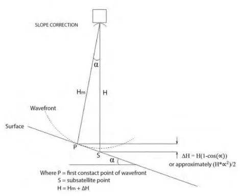
I.6.4 Surface slope effect . . . 40
I.7 The different satellite altimetry missions . . . 41
I.7.1 Topex/Poseidon, Jason-1, Jason-2, Jason-3 . . . 41
I.7.2 ERS-1/2 and ENVISAT . . . 42
I.7.3 SARAL/AltiKa . . . 42
I.7.4 Sentinel-3A . . . 44
II GNSS Reflectometry 45 II.1 Introduction . . . 46
II.2 State of the art . . . 50
II.2.1 Principle of GNSS . . . 50
II.2.2 The ancestor still full of youth: Global Positioning System (GPS) 50 II.2.3 Globalnaya Navigatsionnaya Sputnikovaya Sistema (GLONASS) . 57 II.2.4 New GNSS . . . 58
Contents
II.2.5 The Positioning measurement . . . 61
II.3 Reflection of GNSS signals . . . 65
II.3.1 Multipath . . . 66
II.3.2 Specular and diffuse reflection . . . 68
II.4 GNSS Reflectometry (GNSS-R) . . . 72
II.4.1 GNSS-R measurement technique . . . 72
II.4.2 Reflectometry through opportunity signals . . . 78
II.4.3 Reflectometer with single antenna . . . 83
II.4.4 Application of GNSS-R for altimetry . . . 86
II.5 Conclusions . . . 87
III Validation altimetry on coastal zone: example of the Bay of Biscay 89 III.1 Summary of the article published in Remote Sensing . . . 90
III.2 Article published in Remote Sensing (11 January 2018) . . . 92
IV GNSS Reflectometry for detection of tide and extreme hydrological events: ex-ample of the Socoa (France), Mekong delta and Red River Delta (Vietnam) 121 IV.1 Résumé étendu . . . 123
IV.2 Introduction . . . 125
IV.3 State of the art . . . 129
IV.4 Methodology . . . 131
IV.4.1 Sea surface height (SSH) derived from GNSS-R signals . . . 131
IV.4.2 Analysis of the GNSS-R-based SSH using SSA and CWT methods 137 IV.5 The Socoa experiment . . . 144
IV.5.1 Characteristics of the Socoa study area . . . 144
IV.5.2 Datasets . . . 145
IV.5.3 SNR-based sea surface height variation estimates . . . 147
IV.5.4 Complementary between SSA and CWT method to extract the tides components in GNSS-R signals . . . 149
IV.5.5 Detection the Xynthia storm in the GNSS R signals using SSA and XWT method . . . 151
IV.6 The Mekong delta experiment (Vietnam) . . . 153
IV.6.1 Characteristics of the Mekong delta area and experimental conditions153 IV.6.2 Parameters for SNR signals analyzing . . . 155
IV.6.3 Comparison between the water level derived from GNSS-R and in-situ gauge records . . . 155
IV.7 Red River Delta (RRD) experiment . . . 156
IV.7.1 The study area and datasets . . . 156
IV.7.2 Parameters for SNR signals analyzing . . . 160
IV.8 Conclusions and perspectives . . . 164 IV.9 Revised version of the article submitted at Remote Sensing, special issue
“Remote Sensing of hydrological Extremes”: . . . 166
V Conclusion and perspectives 183
V.1 Conclusion . . . 184 V.2 Perspectives . . . 191
Introduction générale (en français)
L’élévation du niveau des mers, causée par le réchauffement clima-tique de la planète, a et aura un impact considérable sur les terres côtières de faible élévation non seulement en raison de l’accroissement du risque d’inondation/submersion, mais aussi en raison de l’augmentation de la fréquence des évènements extrêmes i.e. tempêtes, surcotes marines (Cooper et al., 2008; FitzGerald et al., 2008; Kirshen et al., 2008). Ces changements impactent déjà diverses régions des conditions climatiques font peser une menace majeure pour la part croissante de la population mondiale vivant dans les régions (Bondesan, 1995; Karim and Mimura, 2008; Tebaldi et al., 2012), ce qui constitue une menace majeure pour la part croissante de la population mondiale vivant dans les régions côtières à quelques mètres au-dessus du niveau de la mer (McGranahan et al., 2007). L’eau de mer envahit de plus en plus la zone côtière, provoquant l’érosion des sols et la salinisation des terres agricoles. Les intrusions d’eau de mer dans les zones humides, et l’augmentation des biseaux salés menacent l’écosystème côtier et induisent une salinisation de plus en plus important des aquifères.
La surveillance des variations du niveau des mers s’est principalement appuyée sur les mesures in situ des marégraphes en zone côtière. Pour cela nombre de marégraphe mondiaux (90 % selon l’UNSECO en 1983) sont basées sur le principe du marégraphe à flotteur placé dans un puit de tranquillisation qui réduit les hautes fréquences et sont souvent étalonnés par une échelle de marée qui est le système le plus ancien et qui préconisé par l’UNSECO, 1985 et le bureau hydrographique international). Lors des périodes récentes de nouveaux types de marégraphe permettent d’avoir une approche plus globale qui intègre non seulement les marées mais aussi d’autres signaux comme l’hydro-isostasie, les surcharges océaniques, les tempêtes, les tsunamis, les charges atmosphériques etc (WOPPELMANN, 1997; Gouriou, 2012). Ces nouvelles familles de marégraphe : sont par ordre chronologique i) le marégraphe à capteur de pression rendus fiables dès 1964 par Eyries ; ii) les marégraphe à sonde aérienne acoustique qui
mesure le temps de parcours aller-retour d’une onde acoustique entre la sonde et la surface de l’eau et qui étaient très en vogue dans les années 80-90 et qui nécessitait aussi un puit de tranquillisation; iii) les marégraphe Radar dont les évolutions récentes sont les capteurs radar à l’air libre qui s’affranchissent du puit de tranquillisation (Woodworth and Smith, 2003). Depuis le début des années 2000 a vu l’avènement des altimètres radar embarqués sur satellite, qui mesurent le temps de trajet aller-retour du satellite à la surface marine, et permettent une cartographie globale des hauteurs océaniques. Autre point important, même si de nombreux marégraphes sont installés près des côtes, il y a encore peu de houlomètres qui permettent d’obtenir des informations sur l’état de mer. Cependant, le coût élevé de ces types d’instruments et les difficultés rencontrées dans la mise en œuvre des mesures en mer ne permettent que des collectes de données spatiales et temporelles limitées.
Cependant au cours du 20ème siècle, les seules mesures régulières de l’environnement côtier sont les séries marégraphiques qui constituent la plus longue série d’observation de la mer connue. Ils fournissent des séries chronologiques des variations du niveau des mers. Ces données ne couvrent pas tous les besoins d’observation de la région et se limitent à la côte.
L’augmentation du nombre d’observations apparaît comme le moyen le plus naturel d’améliorer la connaissance de la zone côtière. C’est pour pal-lier ce manque de données à l’échelle globale qu’à partir des années 2000, s’est développée, une surveillance planétaire grâce à l’altimétrie satelli-taire. La nécessité d’observations plus fréquentes et/ou spatialement plus denses est impérative sur la zone côtière où "s’accumule" environ 70% de la population mondiale.
Observation altimétrique spatiale
Les observations satellitaires se sont fortement développées au cours des années 1990. Le premier altimètre sur Skylab 3 (1973) avait une pré-cision de 0,6 m (Fu et al., 1988; Frappart et al., 2017). Ses données ont été principalement utilisées pour la détermination du géoïde marin. Il a été suivi par les lancements des satellites Geosat (1985-1990) et
ERS-1 (ERS-199ERS-1-2000), puis par le lancement Topex-Poseidon (ERS-1992-2005), qui a ouvert l’ère de l’altimétrie de haute précision, et ces satellites ont mar-qué un tournant dans l’étude des mouvements océaniques. De plus, ces dernières années, les techniques basées sur la télédétection spatiale ont été utilisées pour étudier non seulement les variations des stocks d’eau océaniques mais aussi celles des grands bassins hydrographiques, ce qui a permis d’obtenir des variations spatiotemporelles des stocks d’eaux conti-nentaux. En fournissant des mesures rapides, complètes et répétées de la surface de l’océan, ces données ont véritablement révolutionné l’histoire de l’océanographie physique moderne. Cependant, ces outils, basées sur les outils de la télédétection, présentent une résolution temporelle médiocre et une distance inter-trace généralement assez grande (par exemple, de 315 km à l’équateur pour TOPEX/Poséidon).
Observations du niveau des mers avec le GNSS
Une méthode qui tend à se développer depuis les quinze dernières années est celle qui consiste a utilisé des bouées GNSS qui ont montrer leur utilité pour calibrer et valider les missions d’altimétrie spatiale (M Watson et al., 2004). Un autre avantage de ces bouées c’est qu’elles enregistrent les dif-férentes composantes de la marée, avec une précision centimétrique proche de celle des marégraphes classiques, mais aussi les signaux haute fréquence. Enfin, autre aspect non négligeable elles permettent de s’affranchir de la zone côtière et peuvent être placées en pleine mer ce qui évitera d’inclure les mouvements verticaux de croûte auxquels sont rattachés les marégraphes côtiers (Blewitt et al., 2010). Bien qu’initialement destiné à la naviga-tion et au posinaviga-tionnement, le GPS (Global posinaviga-tioning system), devenu GNSS (Global Navigation Satellite System) avec l’avènement de nouvelles constellation (GLONASS, BEIDOU, GALILEO) a évolué pour être util-isé de manière opportuniste dans de nombreuses autres applications qui utilisent les signaux des satellites GNSS pour déduire d’autres propriétés ou caractéristiques de la Terre, comme l’épaisseur de neige ou l’humidité du sol (Motte et al., 2016). Avec la modernisation et la densification des constellations GNSS on observe une augmentation drastique des signaux
d’opportunité exploitables. La télédétection GNSS, à partir des signaux réfléchis, est un exemple de ces applications qui permettent aussi de re-garder les variations du niveau des mers. Bien que la propagation des tra-jets réfléchis est considérée comme une source d’erreur en positionnement GNSS, elle a aussi pu être utilisée avec succès pour faire de l’altimétrie selon une technique appelée réflectométrie GNSS ou GNSS-R (
Martin-Neira, 1993). Le GNSS-R est un outil de télédétection prometteur qui
répond aux exigences de couverture spatiale élevée, d’un temps de revisite temporel court, d’un faible coût et d’un faible poids car les capteurs GNSS-R sont des systèmes passifs simples et économiques. En océanographie, les informations sur la position de l’antenne/récepteur et les propriétés physiques de la surface réfléchissante peuvent être utilisées pour produire divers paramètres tels que : la rugosité de surface, la hauteur de la surface de l’océan, la vitesse et la direction du vent, les variations de salinités et même d’identifier la glace de mer.
Récemment, avec l’augmentation des phénomènes météorologiques extrêmes et l’élévation du niveau des mers, les populations du monde entier vont être fortement impactées, en particulier celles de la frange côtière. Pour cette raison, la densification des capteurs et des observations est cruciale pour établir des systèmes de surveillance et d’alerte bien structurés, afin d’assurer la sécurité des populations. Dans cette thèse, j’ai combiné l’utilisation d’observations in situ, de mesures altimétriques satellitaires et de données GNSS-R, qui permettent d’établir une couver-ture géographique à différentes échelles depuis la mesure locale jusqu’aux données globales ceci pour une répétitivité temporelle élevée, continue dans le temps, qui sont indispensables pour la surveillance des événements extrêmes, de la dynamique côtière et même des marées si l’on peut extraire les hautes fréquences indépendantes du signal de marée.
Structure de la thèse
Ce manuscrit se compose de 4 chapitres:
général et les différents aspects physiques de la mesure océanique. Les principales missions altimétriques en cours (Topex/Poséidon, ERS-1&2, Jason-1, ENVISAT, Jason-2, SARAL, Jason-3 et Sentinel-3) sont aussi présentées. Ce chapitre se concentre sur l’estimation des niveaux d’eau et présente les limites actuelles de l’altimétrie.
– Chapitre 2 : Le deuxième chapitre se concentre sur l’état de l’art de la technique GNSS-R, et se focalisera plus particulièrement sur les applications de la réflectométrie GNSS pour l’estimation des niveaux d’eau à partir du SNR de récepteurs mono-antenne classique.
– Le troisième chapitre montre une analyse réelle de l’évolution des performances des missions altimétriques, ERS-2, SARAL, etc. pour l’estimation du niveau des mers dans le golfe de Gascogne. Les ré-sultats montrent une nette amélioration de la qualité des données altimétriques SSH dans un rayon de 50 km de la côte voir moins pour les missions les plus récemment mises en orbite, ces résultats sous forme d’article publié dans la revue internationale "Remote Sensing" (Vu et al., 2018).
– Le quatrième chapitre porte sur le traitement des signaux SNR mesurés par une antenne GNSS géodésique pour le suivi des variations des niveaux d’eau sur différents exemple : i) la baie de Socoa (France), ii) delta du Mékong et iii) delta du Fleuve Rouge (Vietnam). Dans ces différents exemples, le signal SNR a été utilisé pour décrypter les signaux des marées et des inondations mais aussi d’évènements extrêmes souvent très rapides.
– Enfin, le cinquième chapitre compile les principaux résultats obtenus dans cette thèse et présente les différentes perspectives offertes par l’altimétrie satellitaire et le GNSS-R.
General introduction (in english)
Rising sea levels, caused by global warming, have and will have a signif-icant impact on low-lying coastal lands not only because of the increased risk of flooding/submersion, but also because of the increase in the fre-quency of extreme events i.e. storms, marine surges (Cooper et al., 2008; FitzGerald et al., 2008; Kirshen et al., 2008). These changes impact al-ready various regions (Bondesan, 1995; Karim and Mimura, 2008; Tebaldi et al., 2012), which constitutes a major threat to the growing share of the world population living in coastal areas a few meters above the sea level (McGranahan et al., 2007). Seawater is increasingly invading the coastal zone, causing soil erosion and salinization of agricultural land. Seawater intrusions into wetlands and increased salt wedges threaten the coastal ecosystem and induce increasing salinization of aquifers.
Monitoring sea level variations has historically been achieved using in
situ measurements of tide gauges in coastal zone. For this purpose, many
of global tide gauges (90% according to UNSECO in 1983) are based on the principle of the float tide gauge placed in a stilling well that reduces high frequencies and are often calibrated by a tidal scale, which is the oldest sys-tem and advocated by UNSECO, 1985 and the International Hydrographic Bureau. In recent periods, new types of tide gauges made it possible to have a more global approach that includes not only tides but also other signals such as hydro-isostasy, oceanic overloads, storms, tsunamis, atmo-spheric loads, etc. (WOPPELMANN, 1997; Gouriou, 2012). These new tide gauge families: are in chronological order i) the pressure sensor tide gauge made reliable by Eyries in 1964; ii) the acoustic aerial probe tide gauge which measures the travel time of an acoustic wave between the probe and the water surface, which was very popular in the 1980s and 1990s and which also required a stilling well; iii) Radar tide gauges whose recent developments are the open air radar sensors which do not require a stilling well (Woodworth and Smith, 2003). Since the early 2000s, al-timetry radar have been developed, which measure the travel time from the satellite to the sea surface and allow global mapping of ocean heights.
Still in modern techniques we can also talk about GNSS buoys which have proven their usefulness in calibrating and validating space altimetry mis-sions (M Watson et al., 2004). Another important point, even though many tide gauges are installed near the coast, there are still few swell that provide information on sea state. However, the high cost of these types of instruments and the difficulties encountered in implementing measure-ments at sea only allow limited spatial and temporal data collection.
However, during the 20th century, the only regular measurements of the coastal environment are the tide gauge series, which constitute the longest known series of observations of the sea. They provide time series of the sea level changes. These data do not cover all the observation needs and are limited to the coast.
Increasing the number of sightings is the most natural way of improving knowledge of the coastal zone. It is to overcome this lack of data on a global scale that from the 2000s, a global monitoring has developed thanks to the satellite altimetry. The need for more frequent and/or spatially dense observations is imperative in the coastal zone where about 70% of the world’s population is "accumulating".
Satellite altimetry observation
Space altimetry observation developed strongly during the 1990s. The first altimeter on Skylab 3 (1973) had an accuracy of 0.6 m (Fu et al.,1988; Frappart et al., 2017). These data were mainly used for the determination of the marine geoid. It was followed by the launches of the satellites Geosat (1985-1990) and ERS-1 (1991-2000), followed by the launch of Topex-Poseidon (1992-2005), which opened the era of high precision altimetry, and these satellites marked a turning point in the study of oceanic displace-ments. In addition, in recent years, remote sensing-based techniques have been used to study not only changes in oceanic water stocks but also those of large continental watersheds, which have resulted in spatio-temporal changes in water stocks of continental waters. By providing rapid, com-plete and repeated measurements of the ocean surface, these data have truly revolutionized the history of modern physical oceanography.
How-ever, these tools, based on remote sensing, have a poor temporal resolution and a generally large inter-track distance (e.g. from 315 km to the equator for TOPEX/Poseidon).
Sea level observations with GNSS
One method that has tended to develop over the past fifteen years is the use of GNSS buoys that have proven useful in calibrating and validat-ing space altimetry missions (M Watson et al., 2004). Another advantage of these buoys is that they record the different components of the tide, with a centimeter accuracy close to that of conventional tide gauges, but also high frequency signals. Finally, another important aspect is that they make it possible to avoid the coastal zone and can be placed in the open sea, which will avoid including the vertical crust movements to which coastal tide gauges are attached (Blewitt et al., 2010). Although originally intended for navigation and positioning, the GPS (Global positioning sys-tem), now GNSS (Global Navigation Satellite System) with the advent of new constellations (GLONASS, BEIDOU, GALILEO) has evolved to be used opportunistically in many other applications that use GNSS satellite signals to infer other properties or characteristics of the Earth, such as snow depth or soil moisture (Motte et al., 2016). With the modernization and increasing amount of GNSS constellations, there is a drastic growth in usable opportunity signals. GNSS remote sensing, based on reflected signals, is an example of these applications that also allow us to look at sea level variations. Although the propagation of reflected paths, known as GNSS reflectometry (GNSS-R), is considered as a source of error in GNSS positioning, GNSS-R has also been successfully used to make al-timetry (Martin-Neira, 1993). GNSS-R is a promising remote sensing tool that fulfills the requirements of high spatial coverage, short revisit period, low cost/low weight systems because GNSS-R sensors are simple, passive and economic systems. In oceanography, antenna/receiver position infor-mation and the physical properties of the reflective surface can be used to produce various parameters such as: surface roughness, ocean surface height, velocity and the direction of the wind, the variations of salinity
and even to identify the sea ice.
Recently, with the increase in extreme weather events, and rising sea levels, people around the world will be heavily impacted, especially those on the coastal fringe. For this reason, the growth of the amount of sen-sors and observations is crucial for establishing well-structured monitoring and warning systems to ensure the safety of populations. In this thesis, I have combined in situ observations, satellite altimetry measurements and GNSS-R data, which allow geographic coverage to be established at dif-ferent scales (from local measurement to global data) with a high tempo-ral repeatability, continuous over time, which are essential for monitoring extreme events, coastal dynamics and even tides if the high frequencies independent of the tidal signal can be extracted.
Thesis Structure
This manuscript consists of 4 chapters:
– Chapter 1: This chapter describes satellite altimetry, its general prin-ciple and the different physical aspects of ocean measurement. The main current altimetry missions (Topex/Poseidon, ERS-1&2, Jason-1, ENVISAT, Jason-2, SARAL, Jason-3 and Sentinel 3) are also pre-sented. This chapter focuses on estimating water levels and highlights the current limitations of altimetry.
– The second chapter focuses on the state-of-the-art of the GNSS-R technique, and will focus more particularly on the applications of GNSS reflectometry for the estimation of water from the SNR of con-ventional mono-antenna receivers.
– The third chapter shows a real analysis of the performance of radar al-timetry from ERS-2 to SARAL in the Bay of Biscay. Alal-timetry-based SSH from former missions was compared to tide gauge measurements acquired along the French Atlantic Coast in the Southern Bay of Bis-cay. The results show a significant improvement in the quality of the altimetry-derived SSH data within 50 km from the coast for the more
recent missions. These results are published in the form of an article in the international journal "Remote Sensing" (Vu et al., 2018).
– The fourth chapter deals with the processing of GNSS SNR signals measured by a geodesic antenna for the monitoring of the variations of the water levels on various examples: i) Socoa Bay (France), ii) the Mekong Delta; and iii) the Red River Delta (Vietnam). In these different examples, the SNR signal has been used to decrypt tide and flood signals as well as extreme events that are often very fast.
– Finally, the fifth chapter complies the main results obtained in this thesis and presents the different perspectives offered by satellite al-timetry and GNSS-R.
Radar Altimetry
Contents
I.1 Introduction . . . 14 I.2 Principle of the Radar Altimeter . . . 15 I.2.1 Estimation of the water height . . . 15 I.2.2 Corrections to the Range . . . 18 I.2.3 Precise orbit determination . . . 22 I.3 Altimeter waveform . . . 22 I.3.1 Waveforms identification . . . 22 I.3.2 Altimeter waveforms over inland waters . . . 24 I.3.3 Altimeter waveforms over coastal domains . . . 26 I.4 Tracking and Retracking . . . 27 I.4.1 Retracking algorithms for the study over inland water . . . 29 I.4.2 Retracking algorithms for the study over coastal areas . . . 32 I.5 SAR altimetry . . . 35 I.6 The limitations of altimetry in coastal areas . . . 37 I.6.1 Waveform retracking problem . . . 37 I.6.2 The stall of the altimeter . . . 38 I.6.3 The correction of the wet troposphere in coastal areas . . . 39 I.6.4 Surface slope effect . . . 40 I.7 The different satellite altimetry missions . . . 41 I.7.1 Topex/Poseidon, Jason-1, Jason-2, Jason-3 . . . 41 I.7.2 ERS-1/2 and ENVISAT . . . 42 I.7.3 SARAL/AltiKa . . . 42 I.7.4 Sentinel-3A . . . 44
I.1. Introduction
I.1
Introduction
The Earth is a complex ecosystem where millions of living species, includ-ing humans, are strongly impacted by the water cycle. This cycle has also an impact on oceans because they cover 71% of our planet. Multiple phys-ical phenomena have a direct impact on our lives and occur on this planet that is constantly evolving. Some these phenomena can rapidly modify its equilibrium such as earthquakes that can cause tsunamis, or on longer time-scale as global warming which has an effect on the increase in the height of the sea surface, ice melting (Mimura, 2013; Senior et al., 2002), natural hazard like earthquakes that can cause tsunamis and the displace-ment of warm oceanic masses that lead to El Niño climatic events. Earth climate is also subject to long-term oscillations such as El Niño Southern Oscillation (ENSO) that has a strong effect on the different fluxes and reservoirs of the global hydrological cycle (Grimm and Tedeschi, 2009; Trenberth and Hoar, 1996). So, in order to study them, we must observe their effects on the ocean surface, which is achieved by the radar altimetry. Indeed, the main goal of radar altimetry is the measurement of the surface topography of the ocean.
An altimeter is a radar instrument that emits electromagnetic (EM) pulse and records the round-trip time, amplitude, and shape of each re-turn signal after reflection on the Earth’s surface. This instrument mea-sures the distance between the satellite and the sea surface. In order to obtain sea surface height (SSH), several corrections to the range due to the atmosphere, the environment, and the instrument need to be taken into account. These measurements are of great importance and intervene in various applications such as sea level changes, geostrophic current de-termination or bathymetry estimates. Since the beginning of the high precision altimetry era, which started in 1991 with the launch of ERS-1, a lot of technical improvements in terms of sensors and orbit determination contributed to higher accuracy of the altimetry-based height estimates.
coast cannot be used, due to the interaction of the radar signal with land topography, inaccuracy in some of the geophysical adjustments and the rapid changes in sea level. In order to optimize the completeness and the accuracy of the sea surface height information derived from satellite al-timetry in coastal ocean areas, the X-TRACK system has been developed by the Center of Topography of the Ocean and Hydrosphere in Toulouse (CTOH - LEGOS) to improve classical altimetry over oceans and land sur-faces (Birol et al., 2016; Stammer et al., 2017) (F. Birol, 2017; Stammer, et al., 2017). Similar, MAPS (Multi-mission Altimetry Processing Soft-ware) is a software developed to process altimetry data on lakes, rivers and flood zones to calculate water time series (Frappart et al., 2015). Cur-rently, MAPs software has been upgraded to improve the quality of the satellite altimetry data on coastal areas as well as land surfaces. We used the MAPs software to process multi-satellite altimetry data for the Bay of Biscay (see in the chapter III).
This chapter, first of all, presents the principle of the radar altimetry and the processing chain to estimate the SSH from the altimetry mea-surements. The characteristics of the altimeter waveforms and retracking algorithms are then described over inland waters and coastal domains. Fi-nally, I will present the various altimetry missions used, in this work, to measure sea surface height.
I.2
Principle of the Radar Altimeter
I.2.1 Estimation of the water height
The principle of spatial altimetry is illustrated in Fig. I.1. The radar altimeter emits an EM pulse towards the ocean surface and measuring their reflections using the backscattering coefficient well-known as sigma nougth (σ0). Altimetry satellites determine the distance between the satellite and the reflecting sea surface, is called range (R), thanks to the two-way travel time of the signal (∆t). The speed of the wave is known (c is the velocity of
I.2. Principle of the Radar Altimeter light) and the round-trip time is measured. It is derived from the equation (Chelton et al., 2001):
R = c.∆t
2 (I.1)
Figure I.1 – Principle of satellite altimetry (Frappart et al.,2017)
The height of the reflecting surface (h) relative to the reference ellipsoid is the difference between the orbital height (H) and the instantaneous height measurements (R):
h = H − R +X
j
∆Rj (I.2)
where ∆Rj is the sum of the instrument corrections, propagation cor-rections, geophysical corrections and surface corcor-rections, which will be presented detail in § II.2. The height h is calculated as the sum of two components: the height of the geoid hg relative to the reference ellipsoid and the average dynamic topography hd. The geoid is a physical equipo-tential surface of terrestrial gravity which corresponds to the average level of the oceans. The average dynamic topography is due to the large and
medium stationary ripples of the ocean surface. The Range (R) is mea-sured from the return echo received by the altimeter. The amplitude and shape of the echoes contain characteristic information of the reflecting sur-face. The area of the intersection of the sea surface and the wave increases to a constant value. The shape of the return pulse is a function of the roughness of the sea surface. Over the ocean, the waveform transmits important information about the state of the sea, such as wave height or speed surface winds (Stammer et al., 2017).
Figure I.2 – Principle of the waveform analysis (CNES)
The diagram in Fig. I.2 shows how the return wave is formed. As the pulse reaches the surface observations, the illuminated surface then increases linearly until a disk-like surface. The power of measurement di-rectly correlated with the illuminated surface. As soon as the impulse enters the ocean, the curvature of the pulses leads to the surface being illuminated in the form of increasingly small surfaces (Fig. I.2 left). The measured power then decreases linearly. In the case of a rough sea surface (Fig. I.2 right), the echo formation mechanism is similar but with weaker ascending and descending slopes. Indeed, the first illuminated surfaces correspond to the peaks of the waves. Gradually, as the pulse illuminates more and more waves, the measured power increases linearly reaching a maximum when the hollows of the waves at nadir (shortest distance be-tween the satellite and the ocean) are illuminated.
I.2. Principle of the Radar Altimeter and the ocean, the altimetry echoes make it possible to determine the average height of the waves taking into account this correlation.
I.2.2 Corrections to the Range
The signals emitted and picked up by the radar cross an environment that is not empty. During its round trip through the atmosphere, some elements such as electrons present, the dry area of the atmosphere and the water vapor, slow down the speed of propagation of the wave and increase the wave path. These phenomena can lead to an overestimation of the range up to 2.5 m. It is, therefore, necessary to apply propagation corrections to obtain a correct determination of the range. In addition, the deformation of the solid Earth is the effect of the attraction of the Moon and the Sun and the variation in the orientation of its axis of rotation, also modify in the precise estimate of the range with an error of the length ∼ 20 cm. These are well-known as geophysical corrections. Some of these corrections are considered directly by the satellite thanks to specific instruments installed on board, other corrections are deduced on the ground using climatological models (Chelton et al., 2001). On the other hand, changes in sea level due to tides or the response to atmospheric pressure must be removed from the altimeter measurement.
I.2.2.1 Propagation corrections
The propagation time of the signal by the altimeter must be best known. However, the radar echo crosses the ionosphere and the troposphere which have a delaying effect on the speed of propagation and lead to systematic errors on the calculated sea level. It is, therefore, necessary to correct the measures of raw distances.
Ionosphere correction: The refraction of EM waves in the Earth’s iono-sphere is caused by the presence of free electrons and ions at altitude above 100 km. These electrons and ions delay the propagation of the EM wave proportionally to the electron density (referred as total electron content or
TEC) in the ionosphere. The diffusion of the radar signal by the electrons contained in the ionosphere can prolong the distance from 2 to 30 mm (Frappart et al., 2006b) depending on the satellite elevation. The iono-sphere range correction is also inversely proportional to the square of the radar frequency (Imel, 1995)
∆Rion = −
kT EC
f2 (I.3)
where k = 0.04025m GHz2 T ECU−1, with the TEC Unit or TECU equals to 106 electrons m−2. This correction can be determined from mea-surements carried out by dual-frequency positioning systems aboard satel-lites, using the difference in the range at the two frequencies provides a noisy estimate of the TEC. This dual-frequency method is used to cor-rect the range for the refraction of the ionosphere over the ocean. Over land and ice sheets, the EM wave can penetrate the surface. The penetra-tion depth is funcpenetra-tion of the nature of the surface and can reach several meters (Chelton et al., 2001).The penetration is also different in the two frequency bands. So, over these surfaces, the difference in range of the two frequencies cannot be used to correct the delay introduced by the iono-sphere. Therefore, the ionosphere corrections to the range are estimated using Global Ionospheric Map model (GIM). These GPS-derived global ionosphere maps (GIM) can be interpolated in space and time to the al-timeter ground track and come close to the accuracy of the dual-frequency altimeters.
The NIC09 ionosphere climatological model is based on the GIMs for 1998–2008 and can also be applied to all single frequency altimeter data prior to 1998 (Scharroo and Smith, 2010)
Another way of estimating TEC is using the Doppler Orbitography and Radiopositioning Integrated by Satellite (DORIS) system, used a mono-free combination of the measurements (pseudo-range or phase) to remove the first order ionospheric effect. However, this method lacks accuracy compared to GIM mode, the production of DORIS ionosphere maps has
I.2. Principle of the Radar Altimeter ceased (Chelton et al., 2001)
Dry troposphere correction: Below the ionosphere, altitude from 0 to 15 km is the troposphere. The permanent gases of the atmosphere (oxygen, nitrogen), modify the atmospheric reflective index and slow down the electromagnetic radiation emitted by the altimeter, causing an error on the altimeter measurement of the order of 2.30 m at sea level. This correction calculated on the ground from meteorological models such as the ECMWF model (European Center for Medium-range Weather Forecast) (Trenberth and Olson, 1988).
Wet troposphere correction: Water vapor content in the atmosphere also causes a slowing down of the radar wave. This effect cause errors of ∼15 cm on the altimeter measurement (Chelton et al., 2001). The value of the correction is determined using the measurements of the radiometer present on board the satellite. Nevertheless, this correction is effective only on the oceans. In fact, on the inland waters and the coastal zones (< 50 km), radiometric data are “polluted” when flying over the land. Conse-quently, the corrections given by the radiometer are useless for calculating the correction of wet troposphere on inland waters and coastal zones. The wet troposphere corrections are therefore deduced from the meteorological models such as the model ECMWF.
I.2.2.2 Instrumental corrections
The quality of the altimeter measurement will also depend on the reliability and the precise determination of the radar measurement. The altimeter range instrumental correction is the sum of the following instrumental corrections (Chelton et al., 2001):
– Doppler correction
– USO (Ultra Stable Oscillator) drift correction
– Internal path delay correction
– Modelled instrumental errors correction
– System bias
I.2.2.3 Geophysical corrections
Geophysical corrections must be added to the range measurement to cor-rect this range due to the tides (ocean, solid earth, polar tides and loading effects).
Solid earth tide: is the response of the solid Earth to gravitational attractions of the Moon and the Sun, this phenomena is known as the solid earth tide. The magnitude of the solid earth tide ranges up to ± 20 cm when using closed formulas as described in (Wahr and et al., 1981; Edden et al., 1973; Cartwright and Tayler, 1971).
Pole tides: The variation of both the solid Earth and the oceans to the centrifugal potential that is generated by small perturbations to the Earth’s rotation axis, produce a signal in sea surface height at the same fre-quency, called the pole tide (Wahr, 1985). The pole tide has an amplitude of 2 cm over a few months.
Rapid fluctuations of the atmosphere: The range is also affected by the load of the atmospheric pressure. For low pressure conditions, the sea level rises, whereas for high pressure conditions, the sea level decreases. This is called inverted barometer effects (IB), any change of atmospheric pressure deforms the sea water/air interface an increase in barometric pressure of 1 mbar corresponds to a fall in sea level of 0.01 m (Wunsch and Stammer, 1997).
I.2.2.4 Sea Surface corrections
The Sea State Bias (SSB) is an altimeter ranging error due to the time-varying physical effect of the sea surface to corresponding wave height and wind speed differences (Chelton et al., 2001; Frappart et al., 2017). This bias consists of three interrelated effects: an electromagnetic bias or radar scattering bias (EMB), a range tracking bias and a skewness
I.3. Altimeter waveform bias. The EMB is physically related to the distribution of the specular facets (Vignudelli et al., 2011). The range tracking bias is related to the tracker used to estimate the significant wave height (SWH) derived from the waveform (Brown, 1977). The elevation skewness bias is the difference between median sea level used median tracker and the real mean sea level.
I.2.3 Precise orbit determination
Satellite orbits reference to an ellipsoid need to be accurately determined using the Precise Orbit Determination (POD) technique based on the force perturbation models on the satellite and tracking systems such as the DORIS tracking system and supplemented by different services of satellite constellations such as GNSS (Frappart et al., 2017). It is an orbitogra-phy and localization system based on a network of 52 beacons distributed around the world and using Doppler measurements related to the move-ment of the satellite in its orbit. The DORIS system is installed on Spot satellites as well as the JASON-1/2, Envisat, Cryosat, AltiKa and the new missions like JASON-3 and Sentinel 3. In addition, GPS and laser positioning systems are also used. The GPS measurements obtained are in-tegrated into an orbit calculation model that restores the distance between the satellite and the reference ellipsoid with an accuracy of a few centime-ters (approximately 2 cm for T/P and JASON-1). It is truly thanks to the considerable reduction in orbit error that altimetry satellites can now measure centimeter variations in ocean or inland water levels (Fig. I.3).
I.3
Altimeter waveform
I.3.1 Waveforms identification
The raw data of altimetry satellites is in the form of wave, it is called a waveform. The magnitude and shape of the waveforms contain infor-mation about the characteristics of the surface are described in the Fig. I.4 (Brown, 1977; Hayne, 1980). From this shape, six parameters can be
Figure I.3 – Error budget for altimeter missions (©LEGOS/CNRS)
Figure I.4 – Theoretical ocean waveform from the Brown model (Brown,1977) and its charac-teristics (©AVISO/CNES)
I.3. Altimeter waveform deduced:
– Epoch at the mid-height (τ ): the position of the mid-power point (knee point) of the waveform at the middle of the analysis window. – The power of the echo (P): the amplitude of the useful signal.
– Thermal noise power (Po): is followed by a rapid rise of returned power called "leading edge", and a gentle and sloping plateau known as "trailing edge".
– Leading edge slope: significant wave height (SWH).
– Skewness: the leading edge curvature
– Trailing edge slope (ξ): related to the deviation from the nadir of the radar pointing.
The shape of the return radar waveform depends on the surface rough-ness function, which can be described as a function of the delay time. Over the ocean, most return waveforms are Quasi-Brown waveform with a shape and stable narrow peak. The treatment of the echoes based on the theoretical waveform given by the Brown model (Brown, 1977; Hayne, 1980; Rodriguez and Martin, 1995; Callahan et al., 2004; Chelton et al., 2001).
I.3.2 Altimeter waveforms over inland waters
Over the inland water, the waveforms are more complex related to slope and roughness surface within footprint, which are classified in 4 cate-gories (MAJ et al., 1986; Guzkowska et al., 1990; Berry et al., 2005): Oceanic (Quasi-Brown model), Quasi-Specular, Broad-Peak and multiple-peak (Fig. I.5a,b,c,d, respectively).
– Oceanic (Quasi-Brown) waveforms (Fig. I.5a) are characterized by leading edge with wide noisy plateau descending. They correspond to reflections on flat surfaces of uniform diffusion and are observed
Figure I.5 – Typical waveform shapes over inland water (modified from (Berry et al.,2005).
over the large lakes, wide rivers or flood plains that the echo is not disturbed by contamination.
– Quasi-Specular waveforms (Fig. I.5b) have a shape vertical leading edge and a rapid decrease of trailing edge. This kind of the waveforms are found on smooth surfaces such as marshes, rivers, or small water bodies.
– Broad peak waveforms (Fig. I.5c) are characterized by slower de-scending trailing edge than quasi-specular waveforms. This category is formed by the water bodies surrounded by low reflecting surfaces (rivers or small lakes).
– Multiple peak waveform (Fig. I.5d): the echoes with several peaks, where each peak corresponds to the reflection from respective areas covered with water (riverbanks, small lakes. . . ).
– Contamination by land also exists but we discuss about these inter-ferences in the following section.
I.3. Altimeter waveform I.3.3 Altimeter waveforms over coastal domains
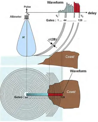
The altimeter waveform in the coastal areas extremely diverse due to the contamination by the vicinity of land (Vignudelli et al.,2011; Gommengin-ger et al.,2011). In the cases of land/sea or sea/land transitions, the num-ber of gates depends on the height and areal extent of the land within the altimeter footprint (Fig I.6).
Figure I.6 – Perturbation of the radar waveform by the emerged lands within the altimeter footprint (© CLS).
Over coastal areas, the altimeter waveforms deviate from the Brown model echo about 10 km from the coast. The waveforms are classified according to their shapes (Fig. I.7). Over 15 km from the coast, between 90% and 95% of waveforms are "Brown" echoes (blue curve). This percent-age rapidly decreases onshore of 15 km from the coastline. Conversely, the percentage of “peak” echoes rises rapidly onshore off 5 km from the coast (pink curve for peak echoes and red curve for the peak with noise in Fig. I.7). Within 10 km from the coast, the waveform shape classes correspond-ing to waveforms with a rise in the trailcorrespond-ing edge (yellow curve) (Vignudelli
Figure I.7 – Percentage of types echoes encountered in offshore environment (modified from (Thibaut,2008)).
et al., 2011).
I.4
Tracking and Retracking
The waveforms are acquired thanks to a tracking system placed on-board the satellite (Chelton et al., 2001). The purpose of the on-board tracker is to keep the position of the middle of the leading edge points to ensure that the echo remains in the reception window. The anticipation system of the measurement makes it possible to minimize the errors. The tracking system is based on the analysis of the parameters of the previous measure-ment points, this system is effective in a homogeneous medium such as the ocean (Brown, 1977). But echo waveforms on others surface such as conti-nental surface include a lot of configurations which are difficult to process, the altimeter is not able to adapt, in real time, these reception parame-ters. A few seconds are needed for the altimeter to find a surface where measurements can resume (Chelton et al., 2001). These few seconds are sufficient to no measurement points are recorded over several kilometers.
I.4. Tracking and Retracking Since JASON-2, tracking systems have evolved and use a digital elevation model (DEM) to open the reception window depending on the altitude of the nadir point over pre-determined zones.
In order to obtain the highest possible accuracy on range measure-ments, the final retrieval of geophysical parameters from the waveforms is performed on the ground, called “waveform retracking”. This reprocessing is based on different algorithms developed according to the nature of the surface overflown (i.e. ice, sea ice). The final range measurement is ob-tained by combining the range of the analysis window (the tracker range) with the retrieved epoch obtained by retracking (the position of the lead-ing edge with respect to the fixed nominal tracklead-ing point in the analysis window) (Vignudelli et al.,2011). According to Brown’s theoretical model (Brown, 1977), the altimetry waveform can be represented by the double convolution between the radar pulse, the response function of a reflective surface element (comprising the antenna gain) and the distribution func-tion of these surface elements. The power received by the altimeter can be represented by (Rodriguez and Chapman, 1989):
Pr(t) = Pe(t) ∗ fptr(t) ∗ ggdf(z) (I.4)
where Pr(t) is the power received by the altimeter, Pe(t) is the transmit-ted power,fptr(t) is the function of response of a reflective surface element (including antenna gain), ggdf(z) is the distribution function of these sur-face elements. This model is based on the following 5 assumptions (Brown, 1977):
1) The diffusing surface is formed of a large number of small independent elements.
2) The statistical distribution of the surface heights is assumed constant over the entire illuminated surface.
3) Diffusion is a scalar process, without polarization effect and indepen-dent of frequency.
depends only on the backscattering cross section and the antenna gain. 5) The Doppler effect is negligible compared to the frequency width of the envelope of the transmitted pulse.
Brown’s model, which theoretically reconstructs the oceanic echo, is the basis of the algorithm used for the treatment of ocean waveforms. After performing the convolution based on the first order Bessel function, the altimeter received power can be expressed as (Deng and Featherstone, 2006): P (t) = PN + 1 2A[erf ( τ √ 2) + 1] exp[−d(τ + d 2)] (I.5)
where PN is the altimeter’s thermal noise, A is the amplitude, t is the time measured, such that t = t0 corresponds to the time arrival of the half power point of the radar return, and σ is the rise time. τ is given as τ = t − t0 σ − d, where d = (δ − β2 4 )σ, and δ = 4 γ c h cos(2ξ); β = 4 γ( c h) 1
2 sin(2ξ), h is the modified satellite altitude, γ is an antenna
beam width parameter, ξ is off-nadir angle.
The analytical expression shown in Eq. I.5 is called the ‘Ocean Model’ which contains five parameters: PN is thermal noise, A is amplitude, σ is rise time, and ξ is off-nadir angle.
I.4.1 Retracking algorithms for the study over inland water
As shown by the results presented in § I.3.2 on the nature of waveforms recorded on inland waters, the radar echoes encountered in the continental domain are very different from those on the ocean. Different reprocess-ing solutions of waveforms have been developed accordreprocess-ing to the surface roughness function considered. The main methods used for the study in the continental domain: the threshold methods, the analytical methods and the pattern recognition methods (Frappart et al., 2006a).
I.4. Tracking and Retracking
I.4.1.1 The threshold methods
– The Ice-1 algorithm: The ice-1 waveform reprocessing algorithm has been developed for the study of polar ice caps, and more generally, continental surfaces. This method based on the principle of thresh-olding, which necessaries the estimation of the amplitude of the wave-form. This technique is known as the OCOG (Offset Centre Of Grav-ity) method developed by Wingham in 1986 (Wingham et al., 1986) should be estimated with the numerical method (Fig. I.8) and is described as follows: COG = Pn=N−aln n=1+aln ny2(n) Pn=N−aln n=1+aln y2(n) (I.6) A = v u u u t Pn=N−aln n=1+aln y4(n) Pn=N−aln n=1+aln y2(n) (I.7) W = ( Pn=N−aln n=1+aln y2(n))2 Pn=N−aln n=1+aln y4(n) (I.8)
Lep = COG − 0.5.W (I.9)
where N is the total gate number; aln is the number of estimated gate in the starting and ending of waveform; y(n) is the value of the nth gate; A is the amplitude; W is the width; COG is the center of gravity of waveform; Lep is the middle point of leading edge.
– The Sea Ice algorithm: is a threshold retracker intended for reprocess the nature of waveforms from sea ice. The amplitude of the waveform is identified: this is the maximum value of the waveform provided by (Kurtz et al., 2014). No model describing the nature of waveforms from sea ice, only a simple method can be used to reprocess this type of radar echoes. The amplitude of the waveform is firstly identified: it is the maximum value of the waveform (Eq. I.10):
Figure I.8 – Schematic diagram of the OCOG algorithm (Wingham et al.,1986).
where y is the value of the nth sample of the waveform and N is the number of sample of the waveform.
I.4.1.2 The analytical methods
– The Ice-2 algorithm: is based on the Brown model (Brown, 1977) to process altimeter waveforms obtained over most of the non-ocean surfaces, intended for ice caps studies, consist in detecting the leading edge width, the trailing edge slope and the backscatter coefficient (Fig. I.9) (Rémy et al., 1997).
– The Ocean algorithm: used to fit a model to measured waveform with a return power model. The waveform shape of an echo is as-sumed to follow the functional form Brown (Brown, 1977; Hayne, 1980). The ocean retracking algorithm objectives is to retrack the waveforms of conventional altimeters by fitting a mathematical model, according an unweighted Least Square Estimator derived from a Max-imum Likelihood Estimator (MLE) method or least squares estima-tors (Amarouche et al., 2004; Thibaut et al., 2010; Vignudelli et al.,