Comparison of parametric methods for modeling corneal surfaces

(1)

PROCEEDINGS OF SPIE

SPIEDigitalLibrary.org/conference-proceedings-of-spie

Comparison of parametric methods

for modeling corneal surfaces

Hala Bouazizi, Isabelle Brunette, Jean Meunier

Hala Bouazizi, Isabelle Brunette, Jean Meunier, "Comparison of parametric

methods for modeling corneal surfaces," Proc. SPIE 10133, Medical Imaging

(2)

Comparison of parametric

methods for modeling corneal surfaces

Hala Bouazizi*

a

_{, Isabelle Brunette}

b

_{, Jean Meunier}

a

_{Dept of Computer Science and Operations Research, University of Montreal}

P.O. Box 6128, Station centre-ville, Montreal, Canada, H3C 3J7;

b

Maisonneuve-Rosemont Hospital

Research Center (Canada), 5415, Boulevard de l’Assomption Montreal, Canada, H1T 2M4.

ABSTRACT

Corneal topography is a medical imaging technique to get the 3D shape of the cornea as a set of 3D points of its anterior and posterior surfaces. From these data, topographic maps can be derived to assist the ophthalmologist in the diagnosis of disorders. In this paper, we compare three different mathematical parametric representations of the corneal surfaces least-squares fitted to the data provided by corneal topography. The parameters obtained from these models reduce the dimensionality of the data from several thousand 3D points to only a few parameters and could eventually be useful for diagnosis, biometry, implant design etc. The first representation is based on Zernike polynomials that are commonly used in optics. A variant of these polynomials, named Bhatia-Wolf will also be investigated. These two sets of polynomials are defined over a circular domain which is convenient to model the elevation (height) of the corneal surface. The third representation uses Spherical Harmonics that are particularly well suited for nearly-spherical object modeling, which is the case for cornea. We compared the three methods using the following three criteria: the root-mean-square error (RMSE), the number of parameters and the visual accuracy of the reconstructed topographic maps. A large dataset of more than 2000 corneal topographies was used. Our results showed that Spherical Harmonics were superior with a RMSE mean lower than 2.5 microns with 36 coefficients (order 5) for normal corneas and lower than 5 microns for two diseases affecting the corneal shapes: keratoconus and Fuchs’ dystrophy.

Keywords: Zernike polynomials, Bhatia-Wolf polynomials, spherical harmonics, 3D shape, parametric model, corneal

topography

1. INTRODUCTION

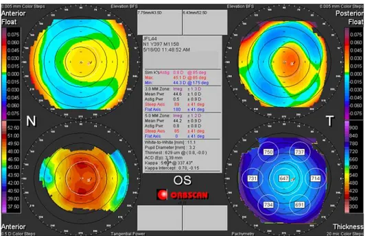
The cornea is the external lens of the eye, and covers roughly one fifth of the eyeball surface, with an average diameter of 11 mm and an approximately spherical shape (figure 1). Models of the cornea have taken many forms, from conceptual models to the schematic eye of Gullstrand to complex computational models that integrate structural, biomechanical and optical representations of the corneal response. The usefulness of any model depends upon valid input, and fortunately recent progress in anterior segment imaging has improved our ability to accurately measure several corneal features. In particular, corneal topography (figures 2 and 3) is a medical imaging technique used to get the precise 3D shape of the cornea as a set of 3D points of its anterior and posterior surfaces. From these data, topographic maps (figure 2) can be derived to assist the ophthalmologist in the diagnosis of disorders. In this paper, we discuss the choice of an appropriate mathematical model to represent the corneal 3D shape. We compare different parametric representations of the corneal surfaces with least-squares fitting (LSF) to the data provided by corneal topography. The small number of parameters obtained with these models reduces the dimensionality of the data from several thousand 3D points to only a few coefficients that could eventually be useful for diagnosis, biometry, implant design etc. Let’s begin with a short review of the mathematical model of the cornea in the literature.

*bouazizh@iro.umontreal.com;

Proc. of SPIE Vol. 10133 101332E-1

(3)

In 2002, Gatinel et al. [1] have reviewed all studies on corneal shape modeling by conic sections including ellipses, hyperbolas and parabolas to model corneal shape. One typical model defines the shape of (a section of) the cornea with only two parameters, which are the apical radius R and its asphericity Q. This was based on the study of Kiely et al. (1984) [2], which describes variations in corneal curvature along any meridian. For a perfect sphere, Q = 0 while a negative value for Q indicates that the corneal surface curvature gradually flattens from center to periphery (prolate shape) and a positive value indicates that the corneal curvature gradually steepens from center to periphery (oblate shape). The apical radius of curvature (R) characterizes the circle tangent to the apex (point of greatest curvature). The smaller the R value, the greater is the curvature, and vice versa. The R and Q values are obtained by least-squares fitting of the following equation to 3D data points (e.g. with corneal topography):

𝑋2_{+ 𝑌}2_{+ (1 + 𝑄)𝑍}2_{− 2𝑅𝑍 = 0 (1)} Gatinel has shown that anterior surfaces have a great variation among individuals. For instance, for aged people, the shape of cornea (anterior surface) becomes more spherical. There is also a little connection between asphericity and ametropia. In progressive myopia, the shape of cornea (anterior surface) becomes more flat or more oblate. For the posterior surface, Gatinel have reported that it can be hyperbolic or prolate. However, this model is not fully 3D because it describes curvature along one meridian at a time or assumes a surface of revolution. Furthermore, although two parameters might be sufficient to describe the global corneal shape, this is somewhat limited to describe the wide variance of corneal shape locally. In 2001, Iskander et al. [3] have shown the interest of modeling cornea with radial functions, especially Zernike polynomials (ZP). These polynomials have been applied to the description of optical aberrations of the Human cornea in 1995 by Schwiegerling [4]. Iskander et al. have also tested Bhatia-Wolf polynomials (BW) [5] which satisfy all the properties of Zernike polynomials and even more. Iskander proposed this approach for the first time in 2002 [6]. Indeed, they found that the BW polynomials performed remarkably well with respect to the Zernike polynomials in terms of the mean square error (MSE) fit. This has been demonstrated for simulated data as well as real data (different corneal data). In 2007, Iskander et al. [7] have tested many mathematics models: simple conics, generalized conics, cosine hyperbolic functions, and a set of fourth, sixth, and eighth radial order polynomials with corneal topography data previously acquired from 92 young adults. In their study, the root-mean-square error (RMSE) between extrapolated topography and true extended topography for various diameters was compared and have shown that extrapolation from central corneal to periphery was best achieved with radial polynomials of the fourth order for normal corneas. In 2009, Iskander proposed for the first time to use Spherical Harmonics SH to model the cornea [8]. They demonstrated that the SH decomposition clearly adjusts the corneal surfaces better than Zernike polynomials with the same number of coefficients (parameters). Zernike polynomials were judged insufficient for the representation of more complex corneal surfaces such as those encountered in post-surgical eyes. They [9] have also compared SH with other 3D radial functions such as hemispherical harmonics and 3D Zernike (3DZ) polynomials and have shown that SH is the best model for the shape of cornea. Finally, in another study, Polette et al. [10] (2014) confirmed the superiority of SH over ZP for a biometrics application. However, all these studies were limited to a relatively small number of corneas and should be analyzed with caution.

Other methods exist to model the cornea, for instance in 2005, Crouch et al. [11] have implemented a finite element model of the eye to investigate factors influencing corneal shape after surgery. These models are useful to simulate the tissue deformation of the eye but are much more complex and not intended for simple parametric modeling of the stationary corneal shape as the previous radial functions. The simple Taylor series [4] also allow decomposing the shape of cornea into simple polynomials but they don't satisfy the condition of orthogonality contrary to radial orthogonal polynomials. Because of the successful results obtained with radial functions in these studies, we will compare them in the present study. An important contribution of this work is the large database used (section 3.1) to correctly estimate the accuracy of each models for both anterior and posterior surfaces.

(4)

Vitreous gel Optic nerve Iris Cornea Pupil Lens Macula Fovea Retina Iris

ô§§ós6"s

_{ó 0 ò ó 0 44 4} s F.

dal

g 4

-éá

.

'i.

.;

-

'.,

E .

y

r, 1""" ,r .:

/ \

. _ .. a E C ó ó 6 rrö _ô qq ó § ó lO q q

8 88 88 88 8888

á á r,

-Figure 1. Cross-sectional view of the eyeball [12]

Figure 2. Typical display of a corneal topographer showing information about the corneal 3D shape. The anterior and posterior elevation with respect to the best fitted sphere (BFS) are shown in the top left and right images while the curvature and pachymetry (thickness) are shown in the bottom left and right images.

2. MATHEMATICAL MODELING OF THE CORNEA

Through the review of the literature, we have seenthat radial functions are the most suitable parametric model for the stationary shape of cornea. We therefore focus our investigation on three types of radial basis functions to fit the shape of normal or abnormal corneas. The first radial basis functions are Zernike polynomials that are typically used in optics. This set of polynomials is defined over a circular domain which is convenient to model the elevation (height) of the corneal surface (provided by the topographer) with respect to a plane perpendicular to the visual axis. A variant of these polynomials, named Bhatia-Wolf polynomials is also investigated. The third representation uses Spherical Harmonics that are particularly well suited for nearly-spherical object modeling, which is the case for cornea. Their formulas are given below.

(5)

2.1 Zernike Z_p(𝑟,θ) = ( √2(𝑛 + 1) 𝑅𝑛𝑚(r) cos(mθ) , p even, m ≠ 0 √2(𝑛 + 1)𝑅𝑛𝑚(r) sin(mθ) , p odd, m ≠ 0 √𝑛 + 1 𝑅𝑛0, m = 0 ) (2)

Where n is the radial degree, m is the azimuthal frequency and 𝑅𝑛𝑚(r) = ∑ (−1)𝑠_{(𝑛−𝑠)!} 𝑠! (𝑛+𝑚 2 −𝑠)!( 𝑛−𝑚 2 −𝑠)! 𝑛−𝑚 2 𝑠=0 𝑟𝑛−2𝑠 (3) 2.2 Bathia-Wolf B_p(𝑟,θ) = ( √2(n + 1) 𝑇𝑛𝑚(r) cos(mθ) , p even, m ≠ 0 √2(n + 1) 𝑇𝑛𝑚(r) sin(mθ) , p odd, m ≠ 0 √𝑛 + 1 𝑇𝑛0, m = 0 ) (4) Where n is the radial degree, m is the azimuthal frequency and

𝑇𝑛𝑚(r) = ∑ (−1)𝑠_{(2𝑛+1−𝑠)!} 𝑠! (𝑛−𝑚−𝑠)!(𝑛+𝑚+1−𝑠)! 𝑛−𝑚 𝑠=0 𝑟𝑛−𝑠 (5) 2.3 Spherical harmonics 𝑌𝑙𝑚(θ, φ) = ( √2𝑁𝑙𝑚 𝑃𝑙𝑚(cos θ) cos(mφ) , m > 0 √2𝑁𝑙𝑚 𝑃𝑙𝑚(cos θ) sin(mφ) , m < 0 𝑁𝑙0 𝑃𝑙0(cos θ), m = 0 ) (6)

Where 𝑁𝑙𝑚 is the normalization factor and 𝑃𝑙𝑚, Legendre polynomial

𝑃𝑙𝑚(x) = (−1)𝑚 2𝑙 _𝑙! (1 − 𝑥 2₎𝑚/2 𝑑𝑙+𝑚 𝑑𝑥𝑙+𝑚(𝑥 2_{− 1)}𝑙₍₇₎

Two other types of mathematical representations centered on the best-fit sphere (BFS) as for SH were not tested here since in [13], Iskander have shown that hemispherical harmonics and 3D Zernike polynomials were less accurate than SH.

3. EXPERIMENTAL RESULTS

3.1 Database

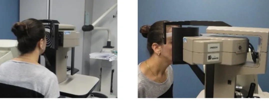
A large dataset of 2392 corneal topographies (anterior and posterior surfaces) were collected using the Orbscan II (Bausch and Lomb, Rochester, NY, USA) topographer (see figure 3). This is a non-invasive device known as corneal topographer used for capturing the shape of cornea. The Orbscan II combines both Placido disc (series of illuminated concentric circles) and slit-scanning technologies, which are captured by a video camera. The resulting data points acquired from each slit are used to reconstruct the true topography of each corneal surface. In less than two seconds, the topographer scans a total of approximately 10,000 3D points. Corneal topography is a recognized technology in the evaluation of corneal shape, curvature and refraction. The Orbscan software calculates a 3D model of the anterior segment and automatically provides many measurements such as elevation (height with respect to a plane perpendicular to the line of sight), pachymetry (corneal thickness), and curvature of the anterior and posterior surfaces of the cornea (see figure 2).

The dataset included 1392 right eye (633 women and 700 men) and 1000 left eye (500 women and 500 men). All of them without any eye disease, surgery or recent contact lenses. The average age was 40±0.2 years, with a spherical equivalent of -3.02±0.03D. Spherical equivalent is negative for myopia and positive for hypermetropia. For abnormal cornea, we have tested 10 cornea with keratoconus and 30 corneas with Fuchs’ dystrophy. Keratoconus is a disorder of the eye which results in progressive thinning of the cornea affecting the shape of the cornea, whereas Fuchs’ dystrophy is a primary

(6)

N

-"

V.

corneal endothelial cell disease that increases corneal thickness. There were three categories of Fuchs according to the severity of the disease: mild (central corneal thickness range: 500–710 µm); moderate (710–775 µm) and severe (775-1100 µm). We compared the 3 different parametric representations of the corneal surfaces with least-squares fitting to the elevation data provided by corneal topography.

Figure 3. The corneal topographer Orbscan II

The corneal shape was recorded as a uniformly spaced 101  101 grid of anterior (and posterior) surface elevations (Z), spaced by 0.1 mm intervals along the X (lateral) and Y (superior-inferior) axes (see figure 4).

Figure 4. Illustration of the corneal surface (anterior or posterior) data representation. One elevation measurement (Z) is shown with a dashed vertical line in a 101 x 101 grid of lateral (X) and superior-inferior (Y) positions.

3.2 Results and interpretation

The mean of RMSE are presented in table 1 for the three models and the three groups (normal, keratoconus and Fuchs) for an approximation with 36 polynomials (corresponding to order 7 for Zernike and order 5 for Bhatia-Wolf and Spherical Harmonics). In this case, the Spherical Harmonics model usually outperformed those of the traditional Zernike and Bhatia-Wolf approximations. These differences were statistically significant with a Z-Test (p-value < 0.01). The RMS error with Spherical Harmonics was near the Orbscan II accuracy reported by the manufacturer (1 micron). One of the claimed benefits of Bhatia-Wolf polynomials is that they provide a richer representation for a given polynomial order; this should produce a better surface model, which was confirmed by our results in figures 5, 6 and 7.

However, for a given order, Bhatia-Wolf requires more polynomials (see figure 11),and to be fair, for the same number of coefficients (same number of polynomials) there was no real advantage of using BW instead of ZP (see Table 1).

(7)

RMSE in microns 12-10 6 4 2 0' 3 4 5 6 7 8 9 10 ' Order

- Zernike

Bhatia - Spherical harmonics RMSE in microns 20 15 10 10 Order RMSE in microns 25 -20 15 lo 5 0' 3 4 5 6 7 8 9 1'0 Order - Zernike Bhatia - Spherical harmonics RMSE in microns 35 30 25 20 15 10

.

5 4 5 6 7 8 9 10 Order

RMSE in microns RMSE in microns

12 10 8 6 4 2 0 Order

-

Zernike Bhatia

-

Spherical harmonics 12 10 8 6 4 2 3 4 5 6 7 8 9 10 10 Order

Table 1 : The mean RMSE in microns for normal and abnormal cornea

Model

Cornea

Zernike

(ZP)

Bathia-Wolf

(BW)

Spherical Harmonics

(SH)

Anterior normal 1.533063 1.653559 1.132959 Posterior normal 2.660893 3.55642 2.289986

Anterior with keratoconus 3.07184585 5.97790501 3.64616391

Posterior with keratoconus 7.01075779 7.37634264 4.97279024

Anterior with mild Fuchs 0.83090856 0.96240747 0.71092733

Posterior with mild Fuchs 2.77481199 3.66542872 2.44206395

Anterior with moderate Fuchs 1.91960848 1.92387002 1.49411479

Posterior with moderate Fuchs 2.44613995 3.52990213 2.62393469

Anterior with severe Fuchs 1.39355265 1.64482837 1.20011593

Posterior with severe Fuchs 2.22905363 3.64616391 2.62764932

Figure 5. RMS error for the shape of normal anterior (left) and posterior (right) corneal surface

Figure 6. RMS error for the shape of anterior corneal surface with Keratoconus (left) and posterior (right) corneal surface

(8)

4 2 0 -2 -4 -4 -2 0 2 4 40 20 -20 4 2 0 -2 -4 -4 -2 0 2 4 40 4v.B) 20 -20 4 -2 -4 -4 -2 0 2 4 30 20 10 o -10 -20 2 -2 -4 -4 -2 0 2 4 40 20 0 -20 4 2 0 -2 -4 Original -4 -2 0 2 4 50 4 2 0 _ 50 -2 -100 -4 -4 -2 0 2 4 20 4 2 -2 -20 -4 -4 -2 0 2 4 -100 4 2 , 0 -2 -4 -4 -2 0 2 4 -1600 .4 4 -2 0 2

z' .e

z' ,e

w

a

70 2 ₂₀ 2 c u

o,

o -Y `. 2 ID

`

-

-2D -1

_ _

-1 -2 0 2

- -2

0 2

1

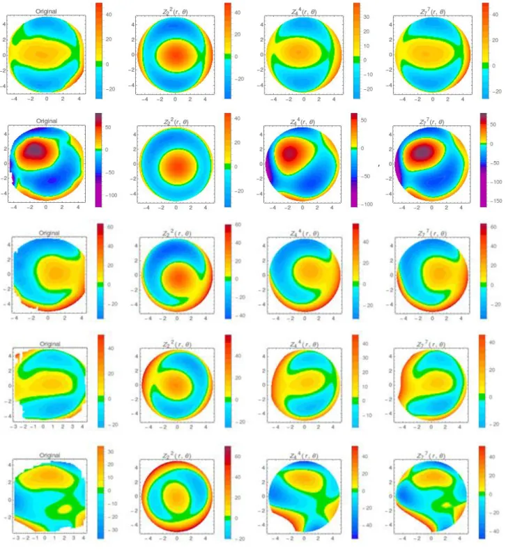
40 20 -3 -2 -t 0 1 2 3 4 4 2 0 -2 -4 -4 -2 0 2 4 40 37 4 20 2 to 0 0 -2 -t0 -4 -4 -2 0 2 4 J 2 -1 0 I 2 7 4 ii t 2 0 _2 -4 -. -2 0 2 4 2 0 2 _4 -2 0 2 40 :o

Figure 8. Topographic map reconstructions for anterior surface with Zernike. From left to right: Original, 2nd, 4th and 7th order. From top to bottom: Normal, Keratokonus, mild, moderate and severe Fuchs.

(9)

4 2 0 -2 -4 -4 -2 0 2 4 4 2 0 -2 -4 -4 -2 0 2 4 4 2 0 -2 -4 -4 -2 0 2 4 4 2 0 -2 -4 -4 -2 0 2 4 -20 4 2 0 -2 -4 Original -4 -2 0 2 4 50 4 0 2 0 -50 -2 -100 -4 -4 -2 0 2 4

:

40 20 -20 -40 2 -2 -4 -4 -2 0 2 4 75 50 4 25 2 0 -2 -25 J -4 -2 0 2 4 50 -50 -100 -150 2 0 _2 -4 4 -2 0 2 2 0 _2 _2 0 2 4 -4 -2 0 2 Y) :L 2 0 -2 _4 _2 0 2 4 2 o -2 -4 -4 -2 0 2 4 4:, -U -fn

Figure 9. Topographic map reconstructions for anterior surface with Bathia-Wolf. From left to right: Original, 2nd_{, 3}rd_and

(10)

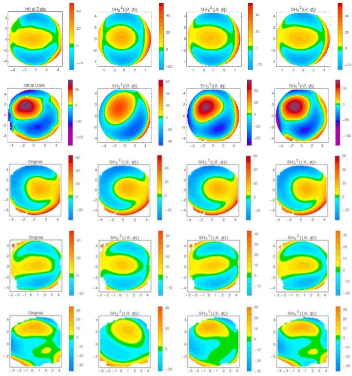
2 -2 - 4 Initial Data -4 -2 0 2 4 4 2 0 -2 -4 -4 -2 0 2 4 SH3300, 4 4 2 2 0 0 -2 -2 -4 -4 -4 -2 0 2 4 -4 -2 0 2 4 4 2 0 -2 -4 Initial Data -4 -2 0 2 4 50 0 -50 -100 4 2 0 -2 -4 -4 -2 0 2 4 60 40 4 20 -20 -40 2 -2 -4 -4 -2 0 2 4 25 4 2 0 -25 -2 -4 -4 -2 0 2 4 50 -100 CC - o z- r z o z-

-

oz-

51::

0 z- 0 o a _ z z 3 -2-1 o t 2 3 di -3 -2 -t 0 I 7 3 4 40 30 4 20 2 t0 ₀ 0 10 _-4 -3 -2 -1 0 1 2 3 4 3 -2 -1 0 1

2 3

)? 20 10 0 -to . 20 .3-2.1 0 1 2 3 4 -3 -2 -1 0 2 3 -3 -2 -1 0 1 2 3 4 20 10 -10 -3 2 -1 0 1 2 3 4 30

p

10 -10 _20

Figure 10. Topographic map reconstructions for anterior surface with Spherical Harmonics. From left to right: Original, 2nd_,

3rd_{and 5}th_{order. From top to bottom: Normal, Keratokonus, mild, moderate and severe Fuchs.}

(11)

1-1

r

L

r

L

,41

r

L

r

.41

r

L

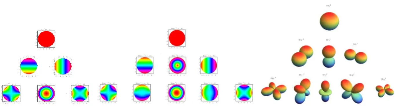
Figure 11. Visual pyramid representation of the Zernike (left), Bhatia-Wolf (middle) and Spherical Harmonics (right) basis functions up to order 2 (Hot colors represent positive values and cold colors, negative values).

Corneas that were diagnosed as keratoconus were more distorted than normal corneas, so, RMS errors were always more elevated for the three models compared with normal ones as expected. However, corneas with Fuchs’ dystrophy generated RMS errors similar and sometimes slightly lower compared with normal ones. This might be due to a more flat surface with the progression of the illness. But in that case, one must be careful with any interpretation since the number of data was limited. Finally, the posterior surface was always more difficult to fit (with higher RMS error) for all models; this might be due to less reliable and noisier data for this surface with the Orbscan II because the posterior surface is the result of a refractive extrapolation of the slit scanning system through the cornea, whereas the anterior surface is directly measured by the slit scanning system combined to a Placido disk analysis [14].

Another way to assess the accurateness of each model is to visually inspect the reconstructed topographic maps with various number of coefficients.Figures 8, 9 and 10show these topographic map reconstructions of each model for the anterior surface of normal, keratokonus and Fuchs’dystrophy. We can appreciate the high quality of the reconstruction with SH.

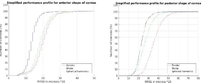
Simplified performance profile [15] (see figure 12) for normal corneas with the three models were also computed. These curves are a straightforward way of comparing methods on sets of problems. Along the x axis, we have the RMSE threshold 𝛼 in microns while for the y axis we show the percentage of fitted corneas that were under this threshold. In other words, the performance profile of a model M is the fraction of the modeled cornea where the performance ratio is at most α. The simplified performance profile is defined as follow:

𝜌𝑀(𝛼) = 1

|𝑐| 𝑠𝑖𝑧𝑒(𝑐 ∈ 𝐶, 𝑅𝑀𝑆𝐸𝐶,𝑀≤ 𝛼) (8) Where 𝜌𝑀(𝛼) is the fraction of the set of corneas (C) well fitted by a model (M) for a RMSE threshold 𝛼.

From figure 12, we note that SH performs the best because its corresponding performance curves are always higher and to the left of the two others. SH achieved 97% of good fitting with 𝛼 = 2 microns for the anterior surface and 99% with 𝛼 = 4 microns for the posterior surface. ZP and BW curves had similar behaviors for the anterior surface but ZP was superior for the posterior surface.

(12)

Simplified performance profile for anterior shape of cornea 110 100 90 80 70 60 50 40 30 -20 10-0 0 ii ii - - -Zemike -Bhatia -Spherical harmonics 10 20 30 40 50 RMSE in microns *10

Simplified performance profile for posterior shape of cornea

110 -100 90 80 70 60 -50 40 -30 20 10 -0 0 - - -Zernike -- -Bhatia -Spherical harmonics 10 20 30 40 50 60 RMSE in microns *10 70 80

Figure 12. Simplified perfermance profile of anterior normal corneas (left) and posterior (right)

To achieve the best performance with SH, we have developped an iterative strategy to fit the model to the cornea. This method is known as Simple Iterative Residual Fitting (SIRF) instead of LSF [16]. In SIRF, we iteratively create an SH model using coefficients up to degree s. In each iteration, we estimate coefficients for one more degree by fitting relevant SHs to the residual. SIRF stops when 𝐿𝑚𝑎𝑥 is reached. Here is the algorithm:

Algorithm: Spherical Harmonics

Step 1: Calculate the best-fit sphere of the corneal surface (BFS). The BFS corresponds to the first harmonics. Step 2: Calculate the residual r between the BFS and the corneal surface

Step 3: For each level l of the SH pyramid: Solve 𝐴𝑙 . 𝑏𝑙= 𝑟

Update the residual r=r- 𝐴𝑙 . 𝑏𝑙 Step 4: m= (𝑟𝑏𝑓𝑠∗ 2√𝜋, 𝑏1𝑇, 𝑏2𝑇, 𝑏3𝑇… , 𝑏𝐿𝑇_𝑚𝑎𝑥) Where 𝐴𝑙 , 𝑏𝑙 and 𝐿𝑚𝑎𝑥 are respectively:

Where 𝐴𝑙 = ( 𝑌𝑙−𝑙(𝜃1, 𝜑1) 𝑌𝑙−𝑙(𝜃1, 𝜑1) … 𝑌𝑙−𝑙(𝜃1, 𝜑1) 𝑌𝑙−𝑙(𝜃2, 𝜑2) 𝑌𝑙−𝑙(𝜃2, 𝜑2) … 𝑌𝑙−𝑙(𝜃2, 𝜑2) . . . 𝑌𝑙−𝑙(𝜃𝑛, 𝜑𝑛) 𝑌𝑙−𝑙+1(𝜃𝑛, 𝜑𝑛) … 𝑌𝑙𝑙(𝜃𝑛, 𝜑𝑛))

𝑏𝑙= (𝑎−𝑙𝑙 , 𝑎−𝑙𝑙+1, . . , 𝑎−𝑙𝑙 ) in which (𝑎𝑙𝑚) −𝑙≤𝑚≤𝑙 are the coefficients given by LSF. 𝐿𝑚𝑎𝑥 is the maximum level to be reached (in our case 𝐿𝑚𝑎𝑥 = 5).

With this method of resolution we constrain the model to have the maximum of shape information in lower levels of the SH pyramid. So, we guarantee that the first coefficient be proportionnel to the BFS radius (commonly used in ophtalmology) and that other (smaller) coefficients represent low frequency deviations from the BFS. Fitting the residual iteratively one level at a time aims to improve the modeling accuracy and creates a better SH model for the corneal surface. To sum up, the key ideas of simple iterative residual fitting (SIRF) includes: (1) instead of solving a large linear system, SIRF solves a series of smaller linear systems iteratively, and the size of the smaller system is controlled by the number of harmonics in each level of the pyramid; (2) SIRF uses multiple passes of LSF to ﬁt the residual, and the number of passes correspond to the the number of levels 𝐿𝑚𝑎𝑥 speciﬁed by a user. This approach is very easy to implement and does not require additional machine resources.

(13)

4. CONCLUSIONS AND FUTURE WORK

To the best of our knowledge this study is the first to use a very large dataset to compare the three most powerful parametric models to fit corneal topographic data. Our results showed that Spherical Harmonics is the method of choice for accurate fitting of normal (or abnormal) corneas with the smallest number of parameters (coefficients of the basis functions). This is also in agreement with the few studies reported in the literature on this topic [3-5]. We have also reconstructed clinical topographic maps for all methods, including Spherical Harmonics for visual inspection and analysis. Our results showed that Spherical Harmonics were superior to Zernike or Bhatia-Wolf parametric models with a mean RMS error lower than 2.5 microns with 36 coefficients (order 5) for normal corneas and lower than 5 microns for keratoconus and Fuchs’ dystrophy (two corneal disorders). Accurate reconstructions of clinical topographic maps are therefore possible with a limited set of 36 parameters with Spherical Harmonics. In the future, we will investigate the use of Zernike polynomial-based rational functions that were shown to outperform traditional Zernike polynomial with the same number of coefficients [9]. We also plan to increase the size of our database of diseases affecting the corneal shape.

REFERENCES

[1] Gatinel, D., Haouat, M. and Hoang-Xuan, T., "A review of mathematical descriptors of corneal asphericity," Journal Francais d'ophtalmologie, 25(1), 81-90 (2002).

[2] Kiely, P., Smith, G. and Carney, L., "Meridional variations of corneal shape," Optometry and Vision Science, 61(10), 619-626 (1984).

[3] Iskander, D., Collins M. and Davis B., "Optimal modeling of corneal surfaces with Zernike polynomials," IEEE Transactions On Biomedical Engineering, 48(1), 87-95 (2001).

[4] Schwiegerling, J., Greivenkamp J. and Miller J., "Representation of videokeratoscopic height data with Zernike polynomials," Journal Of The Optical Society Of America, 12(10), 2105-2113 (1995).

[5] Bhatia, A., Wolf, E. and Born M., "On the circle polynomials of Zernike and related orthogonal sets," Mathematical Proceedings Of The Cambridge Philosophical Society, 50(1), 40-48 (1954).

[6] Iskander, D., Morelande M., Collins, M. and Davis, B., "Modeling of corneal surfaces with radial polynomials," IEEE Transactions On Biomedical Engineering, 49(4), 320-328 (2002).

[7] Iskander, D., Collins M. and Read S., "Extrapolation of central corneal topography into the periphery," Eye and Contact Lens: Science and Clinical Practice, 33(6), 293-299 (2007).

[8] Iskander, D., "Modeling videokeratoscopic height data with spherical harmonics," Optometry and Vision Science, 86(5), 542-547 (2009).

[9] Schneider, M., Iskander D. and Collins M., "Modeling corneal surfaces with rational functions for High-Speed videokeratoscopy data compression," IEEE Transactions On Biomedical Engineering, 56(2), 493-499, (2009). [10] Polette, A., Auvinet E., Mari J., Brunette I. and Meunier J., "Construction of a mean surface for the variability study

of the cornea", Computer and Robot Vision CRV, 328-335 (2014).

[11] Crouch, J.R., Merriam, J.C. and Crouch III, E.R., "Finite element model of cornea deformation," In International Conference on Medical Image Computing and Computer-Assisted Intervention, 591-598 (2005).

[12] National Eye Institute, https://nei.nih.gov/sites/default/files/health-pdfs/factsaboutdryeye.pdf, (22 February 2017). [13] Iskander, D., Collins M. J. and Davis B., "Modeling corneal surfaces with three-dimensional basis

functions," Investigative Ophthalmology and Visual Science, 50(13), 5086-5086 (2009).

[14] Guilbert, E., Saad A., Grise-Dulac, A. and Gatinel, D., "Corneal thickness, curvature, and elevation readings in normal corneas: combined Placido–Scheimpflug system versus combined Placido–scanning-slit system," Journal Of Cataract and Refractive Surgery, 38(7), 1198-1206 (2012).

[15] Moré, J. J., and Wild, S. M. ,"Benchmarking derivative-free optimization algorithms," SIAM Journal on Optimization, 20(1), 172-191 (2009)

[16] Shen, Li., and Moo K. C., "Large-scale modeling of parametric surfaces using spherical harmonics," 3D Data Processing, Visualization and Transmission, Third International Symposium on. IEEE, 294-301 (2006).