Production de monoxyde de carbone dans le système estuarien du Saint-Laurent (Canada)

(1)

UNIVERSITÉ DU QUÉBEC

PRODUCTION DE MONOXYDE DE CARBONE DANS LE

SYSTÈME ESTUARIEN DU SAINT-LAURENT (CANADA)

MÉMOIRE

PRÉSENTÉ À

L'UNIVERSITÉ DU QUÉBEC À RIMOUSKI

comme exigence partielle

du programme de la maitrise en océanographie

PAR

Yong Zhang

(2)

UNIVERSITÉ DU QUÉBEC À RIMOUSKI Service de la bibliothèque

Avertissement

La diffusion de ce mémoire ou de cette thèse se fait dans le respect des droits de son auteur, qui a signé le formulaire « Autorisation de reproduire et de diffuser un rapport, un mémoire ou une thèse ». En signant ce formulaire, l’auteur concède à l’Université du Québec à Rimouski une licence non exclusive d’utilisation et de publication de la totalité ou d’une partie importante de son travail de recherche pour des fins pédagogiques et non commerciales. Plus précisément, l’auteur autorise l’Université du Québec à Rimouski à reproduire, diffuser, prêter, distribuer ou vendre des copies de son travail de recherche à des fins non commerciales sur quelque support que ce soit, y compris l’Internet. Cette licence et cette autorisation n’entraînent pas une renonciation de la part de l’auteur à ses droits moraux ni à ses droits de propriété intellectuelle. Sauf entente contraire, l’auteur conserve la liberté de diffuser et de commercialiser ou non ce travail dont il possède un exemplaire.

(3)

Résumé

Le monoxyde de carbone (CO) joue un rôle important dans le cycle du carbone organique marin. Le CO est produit principalement à la surface de l'océan par photolyse de la matière organique chromophorique dissoute (CDOM). Les flux de photoproduction de CO sont relativement bien connus dans les eaux océaniques, mais reste peu étudiés dans les estuaires et les zones côtières. la production thermique (aphotique) de CO, une autre source potentiellement importante de CO marin, a attiré peu d'attention. Ce travail a examiné les facteurs environnementaux qui influent sur la photoproduction et la production thermique de CO, et évalué les taux de ces deux processus dans un système estuarien de haute latitude-moyenne - Le système estuarien du Saint-Laurent (SLES).

Les effets de la température de l'eau, ainsi que l'origine et l'historique lumineux du CDOM sur le rendement quantique apparent de CO (<Dca) ont été examinés. Le rendement quantique apparent moyen de CO pondéré par l'ensoleillement solaire (<Den) a montré une corrélation linéaire positive avec le coefficient d'absorption normalisé du carbone organique dissous à 254 nm (SUV A254). Le CDOM d'origine terrestre est plus efficace à produire photochimiquement du CO que ne l'est le CDOM d'origine marine. Le photoblanchiment du CDOM a diminué de manière spectaculaire le <Dca pour les échantillons de faible salinité, mais a peu d'effet sur la plupart des échantillons marins. La relation <Dca -T suit un comportement d'Arrhenius. Une équation empirique a été créé pour prédire l'efficacité de la photoproduction de CO dans le SLES en fonction de la température T et du coefficient SUV A254. Sur la base de cette équation et de la

(4)

modélisation du rayonnement solaire sur le SLES, la photoproduction de CO dans le SLES a été estimée à 26.2 Gg CO-C a-I.

Le taux de production thermique de CO (Qco) montrait une corrélation positif et linéaire avec l'abondance de CDOM. Comme pour la photoproduction, la MOD d'origine terrestre est également plus efficace dans la production thermique de CO que la MOD marine. L'influence de la température sur Qco peut être caractérisée par l'équation d'Arrhenius avec des énergies d'activation plus élevées pour les échantillons d'eau douce que pour les échantillons d'eau salée. Qco reste relativement constant entre les pH 4-6, augmente lentement entre les pH 6-8, puis rapidement pour des pH supérieurs. La force ionique et la chimie du fer ont peu d'influence sur Qco. Une équation empirique, décrivant Qco en fonction de l'abondance du CDOM, de la température, du pH et de la salinité, a été construite. En utilisant cette équation, la production thermique de CO dans le SLES a été estimée à 4.2 Gg CO-C a-I.

La production totale de CO dans le SLES est estimée à 30.4 Gg CO-C a-l, avec 86% par photoproduction et 14% par production thermique, indiquant que la photoproduction est la source principale. L'extrapolation de la production thermique aux océans donne 17.1 Tg CO-C a-l, correspondant à 34% de la meilleure estimation disponible de la photoproduction marine de CO. Les concentrations de CO, pour des eaux profondes océanique en régime stationnaire, déduitent de Qco et du taux d'absorption microbien de CO sont de ~ 0.1 nmol L-1; ce qui est consistant avec [CO] d'eaux profondes, déterminées par des méthodes d'échantillonnage sans contamination par du CO et des techniques analytiques.

(5)

Abstract

Carbon monoxide (CO) plays an important role in the marine organic carbon cycle.

CO in the surface ocean is produced primarily from photolysis of chromophoric dissolved organic matter (CDOM). CO photoproduction fluxes are reasonably constrained in open-ocean waters, but remain obscure in estuarine and coastal areas. Thermal (dark) production of CO, another potentially important source of marine CO, has drawn little attention. This work investigated the environmental factors influencing CO photo and dark production and evaluated the rates of these two processes in a high mid-latitude estuarine system- the St. Lawrence estuarine system (SLES).

Effects of water temperature and the origin and light history of CDOM on the apparent quantum yields of CO (<Dca) were examined. The solar insolation-weighted mean apparent quantum yield of CO (<Deo) showed a positive linear correlation with the

dissolved organic carbon-normalized absorption coefficient at 254 nm (SUV A254). Terrestrial CDOM is more efficient at photochemically producing CO th an is CDOM of marine origin. CDOM photobleaching, dramatically decreased <Den for low-salinity

samples, but had little effect on the most marine sample. The <Dca -T relationship followed the Arrhenius behavior. An empirical equation was established for predicting the CO photoproduction efficiency in the SLES from T and SUV A254. Based on this equation and modeled solar irradiance over the SLES, CO photoproduction in the SLES was estimated to be 26.2 Gg CO-C a-l

(6)

The CO dark production rate, Qco, exhibited a positive, linear correlation with the abundance of CDOM. As for photoproduction, terrestrial DOM is also more efficient in CO dark production than marine DOM. The temperature dependence of Qco can be characterized by the Arrhenius equation with the activation energies of freshwater samples being higher than those of saline samples. Qco remained relatively constant between pH 4-6, ascended slowly between pH 6-8 and then rapidly with further

increasing pH. Ionic strength and iron chemistry had little influence on Qco. An empirical

equation, describing Qco as a function of CDOM abundance, temperature, pH and salinity,

was constructed. Using this equation, the dark production of CO in the SLES was estimated to be 4.2 Gg CO-C a-I.

The total CO production in the SLES is estimated as 30.4 Gg CO-C a-l, with 86% from photoproduction and 14% from dark production, indicating that photoproduction is the dominant source. Extrapolation of the dark production to global oceans gives 17.1 Tg CO-C a-l, corresponding to 34% of the best available estimate of marine CO photoproduction. Steady-state deep-water CO concentrations in the open ocean inferred from Qco and microbial CO uptake rates are :<:::; 0.1 nmol L-1, consistent with deep-water [CO] determined with CO contamination-free sampling and analytical techniques.

(7)

List of Tables

Table 3-1 ... 27 Results of Replicate Measurements of <Dco for Stn. Il

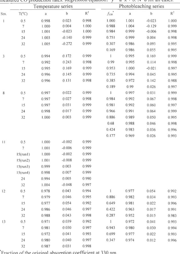
Table 3-2: ... 30 Results from least-squares linear regression between predicted and measured CO production rates. Regression equation: y = a*x + b. N=8 for al! cases

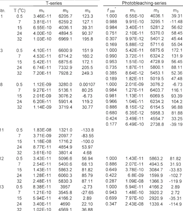
Table 3-3 . ... 33 Fit parameters for function <l>co(À) = ml xexp(m2/(À +m3)) (eq 2-4 in text)

Table 3-4 ... 54 Annual CO photoproduction in the St. Lawrence Estuarine system.

Table 4-1 ... 60 Stations, sampling depth, water temperature (T), salinity, pH, a350, dark production rate

(Qco), and sample storage time.

Table 4-2 . ... 61 Results from least-squares linear regression between CO dark production and incubation time. Regression equation: y = a x x + b. N = 4 for ail cases.

Table 4-3 ... 75,76 Annual CO dark production in the St. Lawrence Estuarine system.

Table 4-4 ... 80 Annual CO dark production in blue waters (water depth >200m).

(11)

(12)

List of Figures

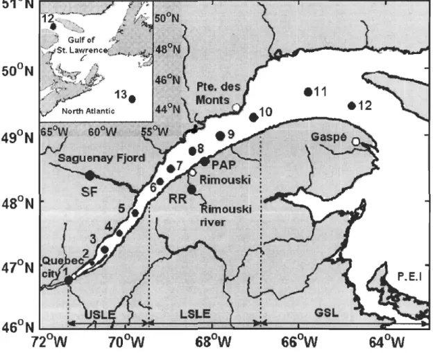
Figure 2-1 ... 8 Sampling locations in the St. Lawrence estuarine system and in the Atlantic Ocean off the Cabot Strait.

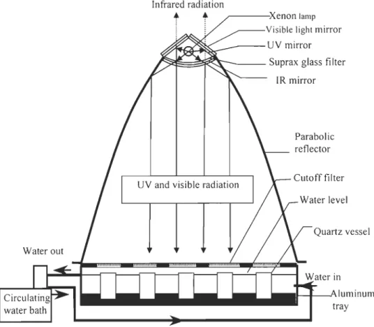
Figure 2-2: ... 11 Cross section of the irradiation system

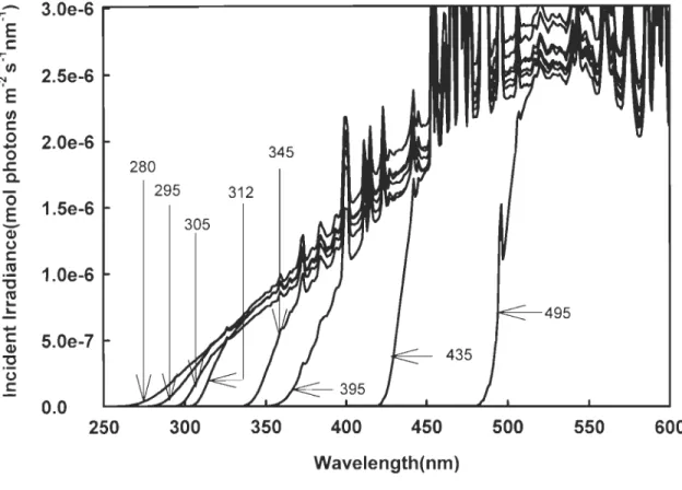
Figure 2-3 ... 13 Incident irradiance in each quartz cell. Numbers at the end of arrows stand for the model of Shott filters above quartz cells.

Figure 3-1 ... 23 Absorption coefficient spectra for the original (pre-faded) samples from Stn.I-13.

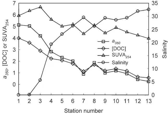
Figure 3-2 ... 24 Distribution of surface-water salinity, absorption coefficient (350 nm, mol), dissolved organic carbon (mg L-'), and specifie absorption coefficient (254 nm, L mg-'m-') along the axial transect in the St. Lawrence estuarine system.

Figure 3-3 ... 25 Plots of a350 (m-'), [DOC] (mg L-'), SUVA254 (L (mgCr' mol), and <Dco vs salinity. The best fit of a350 vs salinity splits into two segments: salinity 0.0043-26.2 (y = -0.116 + 5.02, R2 = 0.995) and salinity 26.2-32.55 (y =-0.267

+

8.86, R2 =0.975). Inset is the <Dco vs SUV A254 plot and the best fit. The <Dco values shown here are those determined at 15 oC on the original (not pre-faded) samples. The 15 oC temperature was chosen since the mean (±s.d.) temperature of the sampled stations was 14.2°C (±4.4°C).

Figure 3-4 ... 28 CO quantum yield spectra of four replicates from Stn Il and their coefficient of variation. Figure 3-5 ... 31

(13)

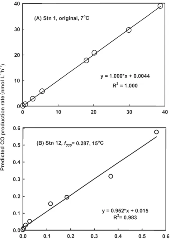
Predicted vs. measured CO production with the best (upper panel) and worst (lower panel) fits.

Figure 3-6 . ... 34 <Dco of Stn. 1 obtained from tempe rature series (upper panel) and photobleaching series measurements (lower panel). Figures in the upper panel are irradiation temperature and 1330 in the lower panel.

Figure 3-7 ... 36,37 Spectral response curves of representative stations (Stns. 1, 8, 12, and 13) and treatments (original vs. photobleached sample).

Figure 3-8 ... 40 Comparison of <Dco spectra for three representative stations in this study with previously published <Dco spectra.

Figure 3-9 ... 43 Arrhenius plots of the solar insolation-weighted mean CO quantum yield, <Dco. Lines are the best fits of the data. Linear regression was not performed for Stn. 13 since its Arrhenius plot is nonlinear.

Figure 3-1 O ... 46 Effect of pre-fading on the CO quantum yields as illustrated by the plots of <Dco vs 1330 (the fraction of the original absorption coefficient at 330 nm).

Figure 3-11 ... 4 7 Effect of pre-fading on the CO quantum yields as illustrated by the plots of <Dco vs the specific absorption coefficient at 254 nm (Stns 1 and 3 only; SUV A254 data for the rest of

the stations are not available).

(14)

<Dco values predicted from eq 3-1 in the main text vs. measured <Dco values. The line is the best least-squares fit of the data.

Figure 4-1A ... 56 Plot of [CO] vs incubation time in the shipboard incubations

Figure 4-1B ... 57 Plot of [CO] vs. incubation time in the [CDOM]-series incubation

Figure 4-1C . ... 58 Plot of [CO] vs. incubation time in the temperature-series incubation.

Figure 4-1D ... 59 Plot of [CO] vs. incubation time in the pH-series incubation

Figure 4-2 ... 64

(A) Dark production rate, Qco, as a function of CDOM absorption coefficient at 350 nm, a350. Line is the best fit of the data; (B) the CDOM-normalized CO dark production rates, /3co (i.e., Qco -:-a350), as a function of salinity, S. Qco was determined at pH

=

7.86 and T = 20°C.

Figure 4-3 ... 66 Arrhenius plots of CO dark production rates. Qco was determined at sample's original pH. Lines are the best fits of the data

Figure 4-4 ... 68 Plots of Qco vs. pH. Qco was determined at 20°C. Lines are the best fits of the data.

Figure 4-5 ... 72

Qco values predicted from Eq. 4-1 in the text vs. measured values. Line is the best fit of the data.

(15)

LOt fAbb

IS

0

reVla Ions an dS

Of

.ym

b 1

os

Symbol Definition Units

<Deo(/') Apparent quantum yield of CO mol CO (mol photonsrl - Solar insolation-weighted mean apparent _mol_C_O₍_{mol photon}_srl <D co _{quantum yield of CO}

/3co [CDOM]-normalized CO dark production rate, nmol L-1 h-I m i.e., QccI' a350)

A wavelength nm

A Cross section of quartz cell ml

A(À) Absorbance at wavelength À

A (2) Absorption coefficient at wavelength À m-I CDOM Chromophoric dissolved organic matter

AQY Apparent quantum yield chl-a ChlorophyIl-a

CO Carbon monoxide

CO2 Carbon dioxide

DIC Dissolved inorganic carbon DOC Dissolved organic carbon DOM Dissolved organic matter

Ea Activation energy J morl

F₃₃₀ Fraction of the original a330 Gg Gigagrams (1 O~ grams) GSL Gulf of St. Lawrence

Qin( À ) incident irradiance mol photons m-2 S-I nm-I

L Pathlength of light m

LSLE Lower St. Lawrence estuary

Pi Measured CO production rate in the itn l -3 -1

irradiation ceIl mo m s

<Pi> Predicted CO production rate in the itn mol m-3 S-I irradiation ceIl

PAP Pointe- au-Pére

Q(À) Photon flux at wavelength À moles photons m-l S-I nm-I Qco Dark production rate of CO nmol _{L- ' h-}I

RR Rimouski River

S Salinity psu

SF Saguenay Fjord

SLES St. Lawrence estuarine system

SUVA254 Specific absorption coefficient at 254nm L (mg

ct

m-I

T

Temperature Kelvin

Tg Teragram(10 Ilgram)

USLE Upper St. Lawrence Estuary

UV-A Ultraviolet radiation between 280-320nm UV-B Ultraviolet radiation between 320-400nm ).lm micrometer

(16)

Acknowledgments

1 thank all the members of my committee for their advice, support and criticism

generously provided throughout this work.

1

am particularly indebted to Huixiang Xie for

identification of a rewarding field of study, and for his encouragement and many

enlightening discussions. Many thanks are extended to S. Bélanger and R. Villeneuve for

measuring CDOM absorbance; A. Rochon for assistance in sample collection; J. Caveen for Matlab programming; G. Canuel for analyzing sali nit y samples; C. Aubry for technical assistance; the scientists, colleagues, and the captains and crew of the Coriolis

Il cruises for their cooperation during the field investigations.

This work was supported by grants from the Natural Sciences and Engineering

Research Council of Canada (NSERC) and the Canada Foundation for Innovation (CFI).

y. Zhang was supported by a Quebec-China Merit Fellowship and an ISMER graduate

(17)

Chapter 1. Introduction

1.1. Significance of CO study

The ocean is a net source of atmospheric carbon monoxide (CO) (Swinnerton et al., 1970; Bates et al., 1995), which regulates the oxidizing capacity of the atmosphere (Derwent, 1995) and acts as an indirect green-house-effect gas that is partly responsible for global warming (Zepp et al., 1998). CO in the surface ocean is produced primarily from the photolysis of chromophoric dissolved organic matter (CDOM) (Conrad et al., 1982; Zafiriou et al., 2003) and is lost by microbial consumption and outgassing (Conrad et al., 1982; Johnson and Bates, 1996; Zafiriou et al., 2003; Xie et al., 2005). Limited data also show that thermal degradation of DOM (Xie et al., 2005). and certain marine organisms (King, 2001) also pro duce CO.

CUITent estimates of the dissolved organic carbon sink associated with DOM photodegradation are 10-30% of total oceanic primary production (Miller and Moran, 1997; Mopper and Kierber, 2000), and are hence clearly relevant on global scales. CO is quantitatively the second largest identified inorganic carbon product of marine DOM photolysis (Mopper and Kierber, 2000). Therefore, CO photoproduction is, by itself, of biogeochemical significance. CO is also considered a useful proxy for general CDOM photoreactivity and for the difficult-to-measure photoproduction of dissolved inorganic carbon (Miller and Zepp, 1995; Johannessen, 2000; Mopper and Kierber, 2000) and biolabile carbon (Kieber et al., 1989; Moran and Zepp, 1997; Miller et al., 2002), which together have been proposed to be one of the major terms in the ocean carbon cycle. Moreover, CO has emerged as a key tracer for use in testing and tuning models of various

(18)

mixed-Iayer processes, including photochemistry, ocean optics, radiative flux, mlxlllg and air-sea gas ex change (Kettle, 1994; Doney et al., 1995; Najjar et al., 1995; Gnanadesikan, 1996; Johnson and Bates, 1996; 2005). Finally, CO acts as a supplemental energy source to sorne lithoheterotrophs, which mediate a major fraction of CO oxidation in ocean surface water (Moran and Miller, 2007). Therefore, any significant advances or modifications in our knowledge of oceanic CO would affect our view of other major marine biogeochemical cycles.

1.2. Existing problems in CO research

Open-ocean CO photoproduction is reasonably constrained (30-90 Tg CO-C a-I )

(Zafiriou et al., 2003; Stubbins et al., 2006a). However, spatial and seasonal variability in the levels, sources and nature of the photoreactant, CDOM, in rivers, estuaries, and terrestrially and upwelling-influenced seas, make photoproduction rates for these aquatic environments hard to predict and, therefore, rates are poorly constrained (Valentine and Zepp, 1993; Zuo and Jones, 1995; Law et al., 2002; Zhang et al., 2006). Estimates of the total marine photoproduction have not advanced in recent years, ranging from 30 to 820 Tg CO-C a-I _{(Valentine and Zepp,}_{1993; Zuo and Jones}_,₁₉₉₅_;_{Moran and Zepp,}₁₉₉₇₎ and only a tentative estimate of global estuarine CO photoproduction exists (-2 Tg CO-C a-I

) (Stubbins, 2001). The significance of CO photoproduction and the uncertainty in current estimates are best illustrated by comparison with other carbon cycle terms. For example, estimates of the total marine photochemical CO source are equivalent to 8-200% of global riverine DOM inputs (Prather et al., 2001) and 16-350% of carbon burial

(19)

In manne sediments (Hedges et al., 1997). These compansons c1early illustrate the importance of CO photoproduction and the requirement to better constrain its potential

contribution to aquatic carbon cyc1ing.

To quantitatively assess the role of CDOM photooxidation in the fate of organic

carbon in the ocean (Miller and Zepp, 1995; Andrews et al., 2000; Vahatalo and Wetzel, 2004), two approaches have been employed most frequently: in situ incubations (Kieber et al., 1997) and optical-photochemical coupled modeling based on apparent quantum

yields (AQYs) (Valentine and Zepp, 1993; Johannessen, 2000; Bélanger et al., 2006). The former determines water column photochemical fluxes by directly incubating water samples at varying depths in the photic zone; it requires laborious fieldwork, but is thought to c10sely simulate the natural photochemistry and the in situ light field. The

latter calculates photochemical rates by combining experimentally determined AQY spectra with CDOM absorption coefficient spectra and underwater irradiance. As CDOM

absorption coefficients can be retrieved from satellite ocean color measurements (Siegel et al., 2002; Bélanger et al., 2008; Fichot et al., 2008), the modeling approach appears

promising for large-scale investigations (Johannessen, 2000; Miller and Fichot, 2006). The reliability of this approach depends, to a large extent, on the reliability of the AQY spectra used in the model. Potentially large uncertainties in published AQY spectra are partly associated with the lack of quantitative knowledge of the influences of CDOM

quality and environmental conditions on the related photoprocesses, inc1uding CO photoproduction.

Thermal (dark) production of CO, another potentially important manne CO source, has so far drawn little attention and its regional and global-scale source strengths

(20)

are unknown. (Xie et al., 2005) observed CO dark formation rates of 0.21 ± 0.21 nmol L-1

h-1 _{in nine cyanide-poisoned Delaware Bay water samples}_. _{Significant CO dark}

production was also inferred from modeling upper-ocean CO cycles (Kettle, 1994, 2005). The dark production term is often critical to rationalize model-data discrepancies and greatly affects the values of CO photoproduction and microbial uptake rates that are derived from inverse modeling approaches (Kettle, 2005). Therefore, the lack of quantitative knowledge of this pathway seriously limits modeling and may add

substantial uncertainties to the global marine CO budget.

It is expected that the distribution and biogeochemical cycling of CO in coastal

(including estuarine) waters would be different from those in the open ocean due at least to 1) coastal waters are highly enriched with DOM relative to blue waters, causing the photochemical depth scale (e.g., e-folding depth oflight at 320 nm) in coastal waters to be smaller than that in the open ocean; 2) coastal DOM is largely of terrestrial origin while DOM in remote-ocean areas is dominantly of marine origin, which could result in different efficiencies of CO production; 3) the far more complex hydrological, physical,

chemical and biological dynamics in coastal zones should give rise to more complicated influences on CO cycling in these areas.

1.3. Objectives

The overall goal of this project alms at improving the estimates of CO source strengths by investigating the CO photo and dark productions in a high mid-latitude estuarine system-the St. Lawrence estuarine system (SLES). This goal will be

(21)

accompli shed through the following specific objectives:

1) To determine the spatial variability of the apparent quantum yield spectrum of CO

photoproduction (C!Jco) and evaluate the effects of water temperature, CDOM's origin and

light history on C!Jco.

2) To determine the spatial variability of the CO dark production (Qco) and assess the effects oftemperature, salinity, pH, and CDOM abundance and origin on Qco.

3) To establish empirical, predictive relationships between C!Jco (and Qco) and relevant environmental variables, such as CDOM absorption, water temperature, pH, and salinity.

4) To model the annual CO photo and dark productions in SLES based on the empirical

equations.

(22)

Chapter 2. Methods

2.1. Study area

The estuary and Gulf of St. Lawrence, referred to as the St. Lawrence estuarine system (SLES) herein, is a semi-enclosed water body with connections to the Atlantic Ocean through the Cabot and Belle-Isle strait (Figure.2-1). It receives the second largest freshwater discharge (600 km3 _a-1

) in North America (Koutitonsky and Bugden 1991; Strain, 1990). Over a relatively small horizontal scale (~1200 km), the SLES provides

various hydrological, geographical and oceanographie features. Surface water in the SLES transitions from freshwater-dominated CASE 2 water in the estuary to oceanic water-dominated CASE 1 water in the Gulf (Nieke et al., 1997). The water column is fairly weil mixed in the upper estuary (Quebec City to the mouth of the Saguenay Fjord) but highly stratified, except in winter, in the lower estuary (the mouth of Saguenay Fjord to Pointe-des-Monts) and the Gulf. An average depth of ~60 m in the upper estuary drops abruptly to >200 m over a few kilometers near the mouth of the Saguenay Fjord (Dickie and Trites, 1983). The typical two-layer estuarine circulation creates a maximum turbidity zone near Île d'Orléans, slightly downstream of Quebec City (d'Anglejan and Smith, 1973). Among the other facets of the SLES are runoff plumes, gyres, fronts, and upwelling areas (Koutitonsky and Bugden, 1991). These features make the SLES an ideal natural laboratory to study the transition of biogeochemical processes from freshwater to estuarine to oceanic water systems.

(23)

2.2. Method for CO photoproduction

2.2.1. Sam pie collection and treatment.

Sampling stations were dispersed along a salinity gradient from the upstream limit

of the St. Lawrence estuary near Quebec City through the Gulf of St. Lawrence and to the

open Atlantic off Cabot Strait. Thirteen stations (Stns. 1-13) were sampled for absorbance

and DOC measurements and six (Stns. 1,3, 8, Il, 12, 13) for the AQY study (Figure

2-l).Water samples (2 m deep) were taken in late July 2004 for Stns. 1-12 and in mid-June

2005 for Stn. 13 using 12-L Niskin bottles attached to a CTD rosette. Samples were

gravity-filtered upon collection through Pail AcroPak 1000 capsules sequentially

containing 0.8 f.1IT1 and 0.2 f.1IT1 polyethersulfone membrane filters. The filtered water was

transferred in darkness into acid-cleaned, 4 L clear glass bottles, stored in darkness at 4

oC, and brought back to the laboratory at Rimouski. Samples were re-filtered with 0.22

f.1IT1 polycarbonate membranes (Millipore) and purged with CO-free air immediately prior

(24)

Figure 2-1. Sampling locations in the St. Lawrence estuarine system and in the Atlantic Ocean off the Cabot Strait.

(25)

2.2.2. Photobleaching

ln order to evaluate the effect of the CDOM's light history on <Dco (i.e., dose dependence), filtered samples, placed in a clear glass container covered with a quartz plate, kept at 15 oC and continuously stirred, were irradiated with a SUNTEST XLS+

solar simulator equipped with a 1.5KW xenon lamp. Radiations emitted from the xenon lamp were screened by a Suprax long band-pass cutoff filter to minimize radiations <290 nm, and the spectral composition of the solar simulator closely matched that of natural sunlight reaching the earth's surface. The output of the lamp was adjusted to 765 W m-2 (280-800nm) at the irradiation surface as determined with an OL-754 UV -vis spectroradiometer (Optronics Laboratories) fitted with an OL IS-270 2 in. integrating sphere. Irradiation time varied from 20 min to 175.0 h to obtain various photobleaching reglmes.

2.2.3. Irradiation for <l>co determination.

The irradiation setup (Figure 2-2) and procedure for determining <Dco spectra were modified from Ziolkowski (2000). Briefly, water samples were purged with CO-free air (medical grade) to reduce the background CO concentration. At the end of purging, they were siphoned through a Teflon tube into pre-combusted (420°C) gas-tight quartz-windowed cylindrical cells (I.D.: 3.4 cm, length: Il.4 cm). The cells were rinsed with the sample water three times and overflowed three times the cell's volume prior to the final filling (without leaving headspace). Then the sample water in quartz cells were irradiated in a temperature-controlled incubator using a SUNTEST CPS solar simulator equipped

(26)

with a 1-k W xenon lamp. Except the top 2-mm sections, the cells were directly in contact

with the cooling solution (a mixture of water and ethylene glycol). The outer sides of the

quartz cells were wrapped in black electrical tape to prevent lateral leakage of radiation between cells. Eight spectral treatments were examined employing successive Schott long band-pass glass filters; their models are (numbers are nominal 50% transmission

cutoff wavelength): WG280, WG295, WG305, WG320, WG345, GG395, GG435, and

GG495). Spectral irradiance under each filter was measured, both before and after sample

irradiation, using the OL-754 spectroradiometer fitted with a 2-inch OL IS-270

integrating sphere. The difference between the two measurements generally was within

1%.

Irradiation time varied from 10 min to 20.0 h, depending on the sample's CDOM

concentration and the filter's cutoff wavelength. The irradiation time was chosen so that

detectable amounts of CO were produced but minimum absorbance losses «4% at 350

nm) were incurred. When significant absorbance losses occurred (3 out of total 456

occasions), the absorbance before and after irradiation were averaged for the calculation of <Dca according to first-order kinetic decay, which well describes CDOM photobleaching

(Del Vecchio and Blough, 2002; Xie et al., 2004). To assess the effect oftemperature on

CO photoproduction, the original samples were irradiated at five temperatures: 0.5, 7.0,

15.0, 24.0, and 32.0°C. Reported irradiation temperatures were post-irradiation

temperatures inside the cells. The dose dependence was evaluated only at 15°C. Thermal

CO production in the parallel dark incubations was on average (± s.d.) 0.33% (± 0.36%)

and 42% (± 21 %) of the production under the WG280 and GG495 filter, respectively. Dark control values were subtracted as blanks.

(27)

Water out

Infrared radiation

t

isible lilght amp mirror ~~~~~_---UV mirror

f')~~~~t----Suprax glass filter

UV and visible radiation IR mirror Parabolic reflector Cutoff filter Quartz vessel ----11---'-\ 1 U min u m

(28)

2.2.4. Calculation of <l>co.

The spectral CO apparent quantum yield, <l>co(À.), is defined as the number of moles of CO photochemically produced per mole of photons absorbed by CDOM at

wavelength À. A Matlab-coded iterative curve fit method (Ziolkowski, 2000; Johannessen

and Miller, 2001) was employed to derive <DeoO.). Briefly, this method assumes an appropriate mathematical form with unknown parameters to express the change in <Deo as a function of wavelength. Decreasing exponential functions are usually chosen for AQY spectra of CDOM photoprocesses (Vahatalo et al., 2000; Ziolkowski, 2000; Johannessen and Miller, 2001). The amount of CO produced in an irradiation cell over the exposure time can then be predicted as the product of the assumed <Deo(..1.) function and the number of photons absorbed by CDOM integrated over the 250-600 nm wavelength range, assuming no CO photoproduction above 600 nm. We followed Hu et al.'s (2002) recommendations to calculate the number of photons absorbed by CDOM at a specifie wavelength À (QCOOM(À)):

aCDOM (À.) -2 -1 -1

QCIJOM(À.)

=

xQi,,(À.)x[l-exp(-aJÀ.)xL)] (molphotonsm s nm ) ... (2-1) a[(À.)

where L is the pathlength of the cells, Qin(À) is the incident irradiance just below the upper window of the cells (Figure 2-3), at (À) is the total absorption coefficient, which is the sum of the absorption by CDOM (acDOM(À)) and water (aw(À)) (no absorption by particles since our samples were 0.2-/..lm filtered). The absorption coefficients of water were taken from Pope and Fry (1997) and Buiteveld et al. (1994).

(29)

~ 3.0e-6 0

E

c: ~ 0 1/) 2.5e-6 ~ E 1/) c: 0 _2.0e-6

-

0 ~ a. 0 1.5e-6 E

-

Q) (.) c: CtI 1.0e-6 "'0 CtI

...

-

c: _5.0e-7 Q) "'0 (.) c: 0.0 250 300 350 400 450 500 550 600 Wavelength(nm)

Figure 2-3. Incident irradiance in each quartz cell. Numbers at the end of arrows stand for

(30)

Using the assumed mathematical form of <l>co (À.) , we can predict the CO production rate

th

in the i irradiation ceIl, <Pi>, to be

< ~ >=

L

-

1

f<l>

co (Â)QCOOM (Â)dÂ (moles m-3 S-I)

(2-2)

À

th

The

l

error between the measured CO production rate (Pi) in the i irradiation cell and the corresponding predicted one «Pi» can be ca1culated as:

x

2

₌

_f[log₍₍_Pi₎_)-log(P)J2

_(2-3)

i=1

The optimum values of the unknown parameters in the assumed <l>co(À.) function are obtained by varymg these parameters from initial estimates until the

l

error was minimized.

The foIlowing quasi-exponential form was adopted to describe the relationship between <l>co and À.:

(2-4)

where ml, m2, and m3 are fitting parameters. This function has been demonstrated to

perform generaIly better (Xie and Gosselin, 2005; Bélanger et al., 2006), particularly in the UV -A and visible wavelengths, than the more frequently used single exponential

(31)

To facilitate analysis of local <Dco variability, we defined a solar spectrum weighted mean CO quantum yield (Bélanger et al., 2006), <D co, over the 280-600 nm range:

<D co = (2-5)

where Q(À) is the noontime cloudless spectral solar photon flux recorded at Rimouski

(48.453~, 68.511°W), Quebec, on 24 May 2005 (Table Al). The rationale for this normalization is to reduce the <Dco spectrum to a single value that accounts for both the magnitudes and shapes of the <Dco (À) and Q(À) spectra, thereby giving more weight to the

wavelengths at which CO production is maximum (i.e., 320-340 nm). From an

environmental relevance perspective, <D co corresponds to the solar insolation-normalized CO production in the water column in which aIl solar radiation over 280-600 nm is absorbed by CDOM. Note that the <D co values presented here are specific to this study since the y more or less depend on the specific Q(À) spectrum used.

2.3. Methods for CO dark production 2.3.1. Sampling

Sampling was conducted aboard the research ship Coriolis 11 between 3-9 May 2007. Four stations (Stns. 1, 3, 4, and 12) were distributed along an axial transect from the upstream limit of the estuary near Quebec City to the Gulf (Fig. 2-1). The same cruise also visited a site in the Saguenay Fjord (Stn SF in Fig. 2-1), an important tributary of the

(32)

SLES with its surface water being highly enriched with CDOM. Water samples were taken using 12-L Niskin bottles attached to a CTD rosette. They were gravity-filtered using sterile Pall AcroPak 500 capsules sequentially containing 0.8-,um and 0.2-,um

polyethersulfone membrane filters. The capsules were connected to the Niskin bottles'

spigot with clean silicon tubing. Prior to sample collection, the capsules were thoroughly rinsed with Nanopure water to avoid potential contamination. The filtered samples were transferred into acid-cleaned 4-L clear-glass bottles or 20-L collapsible polyethylene bags (Cole-Parmer) that were protected against sunlight. Samples in the glass bottles were used immediately upon collection for shipboard incubations. Because of the short duration of the cruise and the constraint on technical resources, those samples in the plastic bags had to be stored in darkness at 4

Oc

and brought back to the laboratory at Rimouski for land-based incubations. Sampling depths for each station visited, along with other related parameters, are shown in Table 4-1.

2.3.2. Contamination assessment

Biological-oxygen-demand (BOD) bottles (300 mL) were used as incubating vessels. Prior to incubations, the BOD bottles were soaked in 10% HCI for over 24 h and rinsed thoroughly with Nanopure water. They were then filled with 0.2 ,um-filtered, CO-depleted Nanopure water and incubated in the dark at room temperatures (~23 OC) for 96 h to check for potential contamination by bottles and filters. The CO formation rates in the bottles ranged -6.4 x 10-5

- 6.8 x 10-5 nmol L-1 h-1, averaged 2.3 x 10-5 nmol L-1 h-1 (± 6.0x10-5 _{nmol L}_-1

_h-

1

, n

=

65), which are negligible compared to the detectable CO production rates in this study.

(33)

A surface (bucket) water sample was collected from the highly colored Rimouski River (Stn. RR in Fig. 2-1) to verify whether sample filtration cou Id cause 10ss of DOM and thus reduce CO dark production. Part of the sample was filtered (0.2 Jll1l) once whi1e the remaining part was filtered twice. The twice-filtered water was incubated in parallel with the sing1e-time filtered water. The two treatments gave essentially identical production values

«0.1

%), proving no significant negative artifacts from filtration. 2.3.3. Shipboard incubations

Shipboard incubations were conducted to measure CO dark production rates, Qco, at in situ temperatures and pH at Stns. 1, 4, 12 and SF. Each sample was purged in the dark with CO-free air (medical grade) to minimize background CO concentration ([CO]),

and then siphoned through a 114" Teflon tube into seven BOD bottles under dimmed room 1ight. The bottles were first rinsed with the sampled water and then overflowed with the samp1e by ~2 times their volumes before the y were closed with no headspace. During the sample transfer, the Teflon tube was inserted nearly down to the bottom of the bottles and bubb1es were avoided. [CO] in one bottle was measured immediately after the sample transfer and subtracted as background [CO] in the later ca1culations. The remaining six bott1es were incubated at constant temperatures (± O.SOC) by immersing them in a darkened circulating water bath. They were sacrificed sequentially for [CO] measurement,

usually at three time points, each in duplicate. 2.3.4. Land-based laboratory incubations

Samples brought back from the Coriolis II cruise were re-filtered with 0.2-Jll1l polyethersulfone membrane filters immediately before the y were incubated. The purposes

(34)

of these incubations was to determine the effects of CDOM concentration ([CDOM]), temperature (T) and pH on Qco. They were performed on water samples from Stns 1, 3, 4, 12 and SF and followed exactly the same procedure as for the shipboard incubations. The [CDOM]-series study was realized by incubating samples from various stations at constant T (20.0°C) and pH (7.86), the median of the samples' original pH values. The T-series incubations were conducted at constant pH (sample's original pH) but at varying T: 2.0, 10.0, 20.0 and 30°C. The pH-series incubations were performed at constant

T

(20.0°C) but at pH varying from 4.0 to 10.0 (Table 4-1). HCI (1 N or 5 N) or NaOH (1 N or 5 N) was used to adjust pH, if required.

The land-based incubations were carried out within 9-26 (average: 19) d of sample collection, with each set of incubation being completed usually within 1-3 d (Table 4-1). An assessment of the effect of sample storage on Qco was conducted on a surface water sample taken from Pointe- Aux-Péres, Rimouski situated on the south shore of the St. Lawrence River (Stn. P AP in Fig. 2-1). Qco (20°C) in this sample was determined, using the same procedure as described above, at storage time of 1, 3, 5, 12 and 22 d. Note that [CDOM]-, T- and pH-series incubations were also performed on the PAP water (Table 4-1).

The effects of ionic strength (I) and iron on CO dark production were investigated using freshly cOllected, filtered RR water. To test the role of ionic strength, varying amounts of NaCI (reagent grade, BDH) were added to aliquots of the water to form an J-series of 0.0, 0.2, 0.4, 0.6 and 1.0 mol L-I

. Samples were then incubated at 20°C. To assess the influence of iron, the water was treated with 100 Jlllloi L-I _deferoxamine mesylate (DFOM) (reagent grade, Sigma-Aldrich), a strong Fe (Zepp et al.)-complexing

(35)

ligand. The water was left in the dark for 24 h to allow the completion of the complexing process before it was incubated (20°C) along with a DFOM-free control. Incubation of Nanopure water spiked with 100 Jll1101 L-1 DFOM did not produce significant CO.

2.4. Analysis.

Samples to be analyzed for CO were brought rapidly to around laboratory tempe rature in a water bath and a sub-sample was drawn from the bottom of the quartz cells or BOD bottles into a 50-mL glass syringe (Perfectum) via a short length of 1/8" o.d. Teflon tubing. The syringe was flushed twice with the sample water before being filled free of bubbles. The sample was analyzed using a headspace method (1:6 gas:water ratio) for CO extraction and a modified Trace Analytical T A3000 reduction gas analyzer for CO quantification (Xie et al., 2002). CDOM absorbance spectra were recorded at room temperature from 200 to 800 nm at 1 nm increments using a Perkin-Elmer lambda-35 dual beam UV -visible spectrometer fitted with 10 cm quartz cells and referenced to Nanopure water. A baseline correction was applied by subtracting the absorbance value averaged over an interval of 5 nm around 685 nm from aIl the spectral values (Babin et al., 2003). Absorption coefficients, aÀ (À: wavelength in nanometers), were calculated as 2.303 times the absorbance divided by the cell's light path length in meters (Johannessen and Miller, 2001). The lower detection limit of the absorption coefficient measurement was 0.03 m-1• This detection limit permitted measuring a at least up to -600 nm for Stns. 1-10 in the estuary (a600: 0.051-0.14 m-1) and up to -500 nm for Stns. 11-13 in the Gulf and Atlantic (asoo: 0.054-0.084 m-1). Dissolved organic carbon (DOC) was measured

(36)

using a Shimadzu TOC-5050 carbon analyzer calibrated with potassium biphthalate. The coefficient of variation (c.v.) on triplicate injections was <5%. Salinity was determined with a Portasal (model 8410A) salinometer. A ThermOrion pH meter (model 420) fitted with a Ross Orion combination electrode was used to determine

pH

;

the system was standardized with three NIST buffers

atpH

4.01,7.00, and 10.01.

(37)

Chapter 3. Photoproduction

3.1. DOM mixing dynamics.

The absorption coefficient for the original (pre-faded) samples from Stns. 1-13 decreased monotonically with increasing wavelength in UV-Visible band (Figure 3-1). Stn. 1 showed the highest absorption coefficient at each wavelength whereas Stn. 13

showed the lowest. The absolute difference among different stations is higher in the UV band and lower in the visible band.

Surface salinity (S) increased from 0.004 at Stn. 1 to 32.55 at Stn. 13. The elevated salinities at Stns. 7 and 9 were likely indicative of recently upwelled waters (Gratton et al., 1988) (Figure 3-2). The DOC and absorption coefficient (a350) distributions nearly mirrored the salinity distribution. The same was true with the DOC-specific UV absorption coefficient at 254 nm (SUV A254), an indicator of the aromatic carbon content of DOM (Weishaar et al., 2003), except at Stns. 2 and 3, where the SUV A254 values were higher than expected considering the salinity distribution trend (Figure 3-2). The SUV A254 vs. S curve (Figure 3-3) further confirms the presence of local DOM sources at these two sites, which are enriched with aromatic carbon relative to the DOM transported from further upstream. Since Stns. 2 and 3 were located in the maximum turbidity zone of the upper St. Lawrence estuary, local DOM inputs cou Id be from the dissolution of trapped particulate organic materials and the injection of DOM into the water column during sediment resuspension. The release of aromatic carbon-rich

(38)

DOM from adjacent mudflats might also have contributed to the high SUVA₂₅_{4 values}

there, especially at Stn. 3.

The a350 value decreased linearly with salinity, but the slope of the line changes at

Stn. 6 (Figure 3-3), slightly downstream from the mouth of the Saguenay Fjord, where

the topography changes abruptly from an average of -60 m in the upper estuary to >200

m in the lower estuary. This a350 distribution pattern agrees with the finding by (Nieke et

al., 1997). Tidal and wind-driven upwelling in and around the he ad of the lower estuary

of CDOM-depleted deep water originating from the Atlantic Ocean (Gratton et al., 1988)

could be mainly responsible for this feature. Relatively more intense in situ

photobleaching in the lower estuary, as expected from the longer residence times of

surface waters there, might also have played a role. However, the linear a350-S

relationship across the entire lower estuary suggests the absence of significant

photobleaching. The [DOC]-S relationship resembles the a350-S relationship except at Stn.

3, where [DOC] is lower than inferred from the DOC mixing line, resulting in the

(39)

25~---~

20

15

_{Stn 12}

-'7

E

Stn 13

-10 5

o

~~~;Iiiiiiii

__

;;:;;=== __

250

300

350

400

450

500 wavelength

(nm)

Figure 3-1. Absorption coefficient spectra for the original (not pre-faded) samples from Stns.l-13.

(40)

7

35

6 ₃₀

'<t LO N

5 ~

25

:::J

₄

Cf)

-e--

_a

350

20

>-"- .-0

3 -+-

[DOC]

c

..--. Ü _~

_SUVA

254

15 cu

0

Cf)

0

2 ...

â

10

1

1.{) C")

co

0

5

0

1

2 3 4 5 6 7 8

9 10 11 12 13

Station number

Figure 3-2. Distribution of surface-water salinity, absorption coefficient (350 nm m-I ),

dissolved organic carbon (mg L-1), and specifie absorption coefficient (254 nm, L

(41)

7 5 6 Y =1.20x -3.50

'b

-

~ 4 R2=e.986 i< 5 0 0

1

6

~ 0 ₄

~ÂL1

ID 3 0 ~

,~

i< 0 (,) 2 le ~ 10

if:

3

•

::J 0

en

3 4 5 6 7 ... ₂ ()

0

SUV~54 Cl ...

X

a350 Ô 1 10

0

[DOC] (') ro

6.

_SUVAzs4 0

-0

<I>co

o

5 10 15 20 25 30 35

Salinity

Figure 3-3. Plots of a350 (in m-1₎_,_[_D_{OC] (in mg L-}1₎_,_{SUVA254 (in L (mgC)-l m-}1₎_,_and

<D co vs salinity. The best fit of a350 vs salinity splits into two segments: salinity 0.0043

-26.2 (y = -0.116

+

5.02, R2 = 0.995) and salinity 26.2-32.55 (y =-0.267

+

8.86, R2 =0.975). Inset is the <D co vs SUV A254 plot and the best fit. The <D co values shown here are

those determined at 15 oC on the original (not pre-faded) samples. The 15 oC temperature

(42)

3.2. Method evaluation for modeling <1>coO,,) 3.2.1. Reproducibility of <1>co(l,,) determination

The reproducibility of the method for determining the <1>coO,,) spectra was

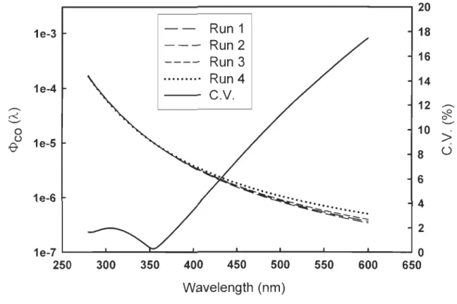
evaluated by running four replicate samples from Stn. Il. The coefficient of variation (c.v.) for CO photoproduction ranges from 1.1 to 12.0%, generally rising with increasing cutoff wavelength (Table 3-1). The <1>coO,,) spectra for these replicate runs are shown in Figure 3-4. The c.v. of the four <1>co(À) spectra is below 2% in the 280-360 nm wavelength range and thereafter increases approximately linearly with increasing wavelength, reaching 17.5% at 600 nm (Figure 3-4). The mean (± s.d.) c.v. across the 280-600 nm range is 7.4% (± 5.6%). The c.v. of <Dco is 4.2% (Table 3-1). The latter is

smaller than the former since the major production of CO occurred in the UV region «400 nm) (see section 3.4.). Note that the performance of this method cannot be effectively evaluated with the c.v. of the individual fit parameters (Table 3-1) since both

the magnitude and shape of the <1>co(À) spectrum is controlled by the combination of the

(43)

Table 3-1. Results of Replicate Measurements of <Dco for Stn. Il

Run No. Statistic results

Cutoff filter 1 2 .) ,., 4 mean s.d. c.v. (%)

CO Photo- _WG280 ₈_.₅₇ ₈_.₇₇ _8.72 _8.62 _8.67 ₀_.₀₉₃ _1.1 production _WG295 _5.1₇ ₅_.₂₅ _5.2 ₅_.₁₂ _5.18 ₀_.₀₅₅ _1.1 rate (nmol L-1 _{h- l)} _WG305 _2.98 _3.02 ₂_.₉₉ _2.93 _2.98 _0.037 _1.₂ WG320 2.51 2.46 2.56 2.57 2.53 0.050 2.0 WG345 0.66 0.67 0.66 0.69 0.67 0.014 2.1 GG395 0.37 0.38 0.36 0.37 0.37 0.0093 2.5 GG435 0.1 0.1 0.09 0.1 0.10 0.0037 3.8 GG495 0.02 0.02 0.02 0.02 0.02 0.0023 12.0

Fitting _ml ₁_._18E_-_{08 1}_.₀₂_E_{-08 1.56E}_-_{08 3. 13}_E_{-08 1}_.₇_2E_-_{08 9}_._64E_-₀₉ ₅₆_.₀

parameters _m₂ ₁₇₁_6.2 ₁₇_61.6 _1591.3 ₁₃₁₂_.₆ _1595.4 ₂_01.8 ₁₂_.₇

of <Dco().,,)

m3 -100.03 -98.79 -108.70 -127.04 -108.64 13.04 -12.0

(44)

20 1e-3 Run 1 18

---

Run

2

- - - - _Run₃ 16

...

_{Run 4} ₁₄ 1e-4

C.v.

.- 12 .-c< ";$? ₀ -.- -.-0 10

>

ü 1e-5

e-

₈ ü 6 ~ 1e-6 .~

...

₄ eiiiiii;..._ •••••• ~

...

~: 2 1e-7 0 250 300 350 400 450 500 550 600 650 Wavelength

(nm)

Figure 3-4. CO quantum yield spectra of four replicates from Stn. Il and their coefficient of variation.

(45)

3.2.2. Performance of the curve fit method

The performance of the curve-fit method for deriving <Dca was evaluated

according to the approaches of Ziolkowski (2000) and Johannessen and Miller (2001). First, the <Dca spectra derived from the curve-fit method, in conjunction with the relevant irradiance (Figure 2-3) and CDOM absorbance spectra, were used to calculate the CO production rates in the irradiation cells. Then, the calculated (or predicted) rates were

plotted against the CO production rates measured in the corresponding cells, and linear

regressions were performed between the two. Results from the linear regression were shown in Table 3-2. R2 shows how weIl the predicted rates correlate with the measured

rates. Of the total 57 runs, 19 reached R22: 0.999, 18 R20.997-0.998, 10 R20.994-0.996,

(46)

Table 3-2 : Results from least -squares linear regresslOn between predicted and

measured CO production rates. Regression equation: y = a*x

+

b. N=8 for aU cases. Temperature series Photobleaching series

SIn. T(°C) a b R2 /330

.

a b R2 0.5 0.998 0.023 0.998 1.000 1.001 -0.023 1.000 7 1.000 0.004 1.000 0.988 1.004 -0.129 0.999 15 1.001 -0.023 1.000 0.984 0.999 -0.006 0.998 24 1.003 -0.140 0.999 0.751 0.999 0.004 0.998 32 1.005 -0.272 0.999 0.307 0.986 0.093 0.995 0.169 0.986 0.055 0.995 3 0.5 0.994 0.172 0.999 1 0.995 0.169 0.999 7 0.992 0.243 0.998 0.99 0.995 0.114 0.998 15 0.995 0.169 0.999 0.953 1.000 -0.021 0.997 24 0.996 0.145 0.999 0.735 0.994 0.045 0.995 32 0.996 0.131 0.998 0.385 0.972 0.142 0.988 0.189 0.99 0.026 0.997 8 0.5 0.997 0.022 0.999 1 0.997 0.031 0.999 7 0.997 0.027 0.998 0.984 0.992 0.067 0.998 15 0.997 0.031 0.999 0.981 0.992 0.060 0.997 24 0.998 0.017 0.999 0.966 0.991 0.064 0.999 32 1.000 0.003 0.999 0.886 0.989 0.050 0.995 0.68 0.988 0.046 0.998 0.424 0.983 0.036 0.996 0.177 0.969 0.026 0.993 Il 0.5 1.000 -0.002 0.999 7 1.001 -0.006 0.999 15(runl) 1.000 -0.002 0.999 15(run2) 1.001 -0.008 0.999 15(run3) 0.999 0.003 0.999 15(run4) 0.998 0.007 0.999 24 0.994 0.005 0.990 32 1.004 -0.048 0.997 12 0.5 0.978 0.043 0.994 1 0.977 0.054 0.992 7 0.979 0.046 0.995 0.886 0.982 0.034 0.993 15 0.977 0.054 0.992 0.649 0.981 0.022 0.996 24 0.986 0.046 0.997 0.422 0.963 0.017 0.991 32 0.988 0.043 0.998 0.287 0.952 0.015 0.983 13 0.5 0.971 0.039 0.992 0.972 0.041 0.993 7 0.981 0.030 0.997 0.943 0.980 0.030 0.994 15 0.972 0.041 0.993 0.699 0.977 0.022 0.993 24 0.980 0.040 0.997 0.347 0.974 0.012 0.996 32 0.987 0.031 0.998

(47)

....

J::

....

~ (5 E c: '-' Cl)

-

ni

...

c:

o

:o::i o ;:, "C o

...

Co

o

U "C Cl)

-

o "C Cl)

...

Cl. 40~---~~

30

20 10 (A) Stn 1, original, 7°C

y

=

1.000*x + 0.0044 R2

=

1.000 Ol~~---~---~---~---~

o

10 20

30

40

0.6 - - - 0 - - - - .

0.5 0.4

0.3

0.2 0.1 (B) Stn 12, '330= 0.287, 15°C y

=

0.952*x + 0.015

R

2

=

_0.983

O.O\Y---""---... ---"""---'

_0.0

0.1 0.2

0.3

0.4 0.5

0.6

Measured CO production rate (nmol L-1 h-1)

Figure 3-5. Predicted vs. measured CO production with the best (upper panel) and worst

(48)

3.3. <1>co{J,,) spectra

A compilation of the fit parameters for <1>co(À) is shown in Table 3-3. Ali <1>co(À)

spectra are similar in shape. <1>co(À) decreased with wavelength, increased with

temperature, and for most stations decreased with the extent of photobleaching (f330). Representative <1>co(À) spectra at Stn. 1 are shown in Figure 3-6.

(49)

Table 3-3. Fit parameters for function <l>coOI.) = ml xeX.Q(m2/(À+m3)) (eq 2-4 in the text) T-series Photobleaching-series T (oC) _f₃₃₀

.

Stn. m1 m2 m3 m1 m2 m3 1 0.5 3.46E-11 6205.7 123.3 1.000 6.55E-10 4036.1 39.31 7 3.81E-11 6259.2 127.1 0.988 9.91E-10 3295.1 -11.48 15 6.55E-10 4036.1 39.31 0.984 3.40E-11 5281.2 56.62 24 4.00E-10 4894.5 90.37 0.751 2.10E-11 5370.0 58.45 32 1.03E-10 6969.1 195.8 0.307 9.97E-12 5401.2 45.44 0.169 5.88E-12 5711.6 55.04 3 0.5 4.10E-11 6600.9 151.9 1.000 5.42E-11 6875.6 172.1 7 4.53E-11 6714.2 160.2 0.990 3.72E-11 6324.2 131.9 15 5.42E-11 6875.6 172.1 0.953 1.51E-10 4728.9 56.45 24 6.74E-11 7332.9 205.5 0.735 1.87E-11 5800.1 88.11 32 7.20E-11 7928.2 249.3 0.385 8.64E-12 5453.1 52.36 0.189 1.82E-11 5019.5 47.48 8 0.5 1.12E-09 3280.0 0.00107 1.000 2.01 E-09 3076.2 -6.73 7 9.27E-11 5136.1 80.25 0.984 1.27E-11 6403.7 116.1 15 2.01 E-09 3076.2 -6.73 0.981 1.13E-11 6069.5 93.39 24 6.20E-11 5901.4 119.2 0.966 1.04E-11 6234.2 104.2 32 1.14E-09 3719.4 30.77 0.886 8.15E-12 6154.5 96.88 0.680 6.35E-12 5958.3 81.88 0.424 3.49E-11 4554.7 33.25 0.177 6.49E-10 2738.8 -39.19 11 0.5 1.83E-08 1321.0 -133.8 7 3.71 E-09 2097.7 -83.55 15 1.18E-08 1716.2 -100.0 24 8.77E-11 4854.9 53.97 32 3.61 E-10 3801.4 4.68 12 0.5 3.43E-11 5096.6 56.94 1.000 1.43E-11 5863.2 81.82 7 2.54E-11 5400.6 68.13 0.886 2.07E-11 4943.5 31.93 15 1.43E-11 5863.2 81.82 0.649 3.78E-10 3084.7 -33.83 24 1.28E-11 6060.3 85.79 0.422 6.8E-09 1599.9 -102.7 32 2.48E-11 5830.3 87.11 0.287 1.09E-08 1366.3 -119.9 13 0.5 8.38E-11 3957 -2.73 1.000 5.94E-11 4166.2 2.89 7 1.21 E-10 3545.8 -27.65 0.943 1.48E-10 3920.2 2.72 15 5.94E-11 4166.2 2.89 0.699 7.97E-10 2920.9 -35.31 24 3.40E-11 4690 22.10 0.347 2.43E-08 1339.4 -114.9 32 1.02E-10 4569.1 36.88 * Fraction of the original a330 values. The original Q330 (m-l) values are 6.33 (Stn. 1),6.37 (Stn. 3),2.6 (Stn. 8), 1.2 (Stn. Il),0.61 (Stn. 12), and 0.38 (Stn. 13).

(50)

1e-3

~---. Temperature series

1e-4

₃₂

_.

₀

_Oc

24 .

0 Oc

15 .

0 Oc

1e-5

1e-6

o

1e-7

~~---~----~---~---~----~---~ o

300

350

400

450

500

550

600 1e-3

r---~ Photobleaching series

1e-4

1e-5

1e-6

1e-7

1e-8

L-~ ______ ~ ____ ~ ______ ~ ______ ~ ____ ~ ______ ~

300

350

400

450

500

550

600

Wavelength (nm)

Figure 3-6. <Dco spectra at Stn. 1 for temperature series (upper panel) and photobleaching series (lower panel). Numbers are irradiation temperatures (upper panel) and /330 (lower panel).

(51)

3.4. Response spectra of CO photoproduction

The spectral response of CO photoproduction is defined as the cross product of Q(À) and <l>co(À), where Q(À) is the noontime cloudless spectral solar photon flux recorded at Rimouski (48.453°N, 68.511°W), Quebec, on 24 May 2005 (Table Al). The response curve reflects the spectral distribution of depth-integrated CO photoproduction in the water column, assuming that aU photochemicaUy active solar radiations reaching the sea surface are absorbed by CDOM.

The response curves (Figure. 3-7) for varying locations (terrestrial vs. marine) and treatments (temperature variation and photobleaching) are similar in shape, with a main

peak at ca. 333 nm and a minor peak at ca. 406 nm. One notable feature for Stn. 13 (the

most marine sample) is that relatively more CO was produced in the visible wavelengths

(52)

2.0e-7 , . . . . - - - ,

Stn 1

1.6e-7

- - Original, 15°C

- -

'330=0.169, 15°C

1.2e-7

_{Original, 0.5}

Oc

-"7

_8.0e-8

E

c

"7 ~ ~

_4.0e-8

E

0

E

-

_c

0.0

0

300

350

400

450

500

550

600

~ (,) :::l

1.6e-7

"C 0 ~

a.

0

Stn 8

~ 0 ~

_{Original 15}

Oc

(L

_1.2e-7

0 - - '330=0.177,15

Oc

u

~

Original, 0.5

Oc

8.0e-8

300

350

400

450

500

550

600 Wavelength (nm)

Figure 3-7.Spectral response curves of representative stations (Stns. 1, 8, 12, and 13) and

(53)

1.2e-7 . - - - ,

Stn 12

8.0e-8

Original, 15°C

- - '330=0.287, 15

Oc

-,~,",,,

Original, 0.5

Oc

-":"

E

_4.0e-8

c

":"

.c

~

E

0

E

0.0 -

c

₃₀₀

₃₅₀

₄₀₀

₄₅₀

₅₀₀

₅₅₀

₆₀₀

0 :.; (,J ::::s

8.0e-8

"'C 0 '-c-

_{Stn 13}

0

-

0

.c

6.0e-8

Original, 15°C

a.

0 _{- - '330=0.347,15}

Oc

()

Original, 0.5

Oc

4.0e-8

2.0e-8

0.0

300

350

400

450

500

550

600 Wavelength (nm)

Figure 3-7. (continued)

(54)

3.5. <l>co of terrestrial vs. marine eDOM.

<l>co spectra representative of the upstream limit of the St. Lawrence estuary (Stn. 1), the Gulf (Stn. Il), and the Atlantic Ocean (Stn. 13) are displayed in Figure 3-8. Across the UV -visible regimes, the freshwater had the highest <l>co values, the open-ocean

water the lowest, and the Gulf water intermediate. However, the differences between

these spectra progressively diminished with decreasing wavelength, a pattern in

accordance with previous <l>co spectra determined on water samples from widely varying

geographic regions (Figure 3-8). These observations suggest the presence of multiple CO

precursors that were less selectively photolyzed by UV -B radiation than by UV -A and

visible radiation. It is also possible that metal ions (e.g., iron and copper), which are

known to promote photodegradation of CDOM, could have played a role in this

phenomenon since the concentrations of these metal ions are usually higher in hig h-CDOM estuary waters than in oceanic waters.

The spectra for the Gulf of St. Lawrence and the Atlantic Ocean almost perfectly

match those for the Gulf of Maine (Ziolkowski, 2000) and the Pacific Ocean (Zafiriou et

al., 2003), respectively. Nevertheless, The <l>co values for the freshwater sample (Stn. 1)

from the head of the St. Lawrence estuary are considerably lower, particularly in the U

V-A and visible spectral regions, than those for the more colored inland lake and river waters studied by Valentine and Zepp (1993). This indicates that CDOM photoreactivity can vary substantially among freshwater ecosystems, likely due to differences in the quality of the CDOM. For example, SUVA350 (i.e., a350/[DOC]) for Valentine and Zepp's

(55)

<D co, as defined in eq. 2-5, increased seaward initially (from Stn. 1 to Stn. 3) but

decreased monotonically with salinity downstream of Stn. 3 (Figure 3-3). Since the water mass characteristics in the Gulf are typical of Case 1 waters of oceanic origin (Nieke et al., 1997), the <D co-S relationship demonstrates that marine algae-derived CDOM is less

efficient than terrestrial CDOM at producing CO photochemically. A linear regression reveals that <D co correlates weIl with SUV A₂₅₄ (inset in Figure 3-3); the negative

intercept suggests that not aU aromatics are CO precursors. This <D co -SUV A254

correlation points to an important role of aromaticity in controlling <D co, which is in line

with the study of Hubbard et al. (2006) demonstrating that many specific aromatic compounds are efficient CO producers. As terrestrial DOM usually contains a greater fraction of aromatic carbon than does marine DOM (Benner, 2002; Perdue and Ritchie, 2003), the higher CO production efficiency of terrestrial DOM observed in the present study is likely a general feature for aquatic environments. Mopper et al. (2006) found that increasing salinity reduced the photoreactivity of a high-CDOM swamp sample, inc1uding CO photoproduction. However, as SUV A254 could account for 98% of the variance of <D co (Figure 3-3), salinity was probably not a prevailing determinant of <D co

(56)

1e-3

~---,

• Average Pacific blue water

1e

-

4

• Ave

r

age freshwater

1e

-

5 • •

•

0

e

1e-6

_{Gulf of Maine}

(Grey line)

1e-7

Stn 13 Stn 11 (black line)

1e-8

250

300

350

400

450

500

550

600

650 Wavelength (nm)

Figure 3-8. Comparison of <Dco spectra for three representative stations in this study with previously published <Dco spectra. The <Dco spectrum for average freshwater is from Valentine and Zepp (1993), for the Gulf of Maine from Ziolkowski (2000), and for average Pacific blue water from Zafiriou et al. (2003). The spectra from this study were those determined at 24 oC on the original samples. The 24 oC temperature was chosen since irradiations for the previous studies were performed at room or laboratory temperatures (Ziolkowski, 2000, Zafiriou et al., 2003). The temperature was not reported in Valentine and Zepp (1993).

Production de monoxyde de carbone dans le système estuarien du Saint-Laurent (Canada)

UNIVERSITÉ DU QUÉBEC