Science Arts & Métiers (SAM)
is an open access repository that collects the work of Arts et Métiers Institute of Technology researchers and makes it freely available over the web where possible.
This is an author-deposited version published in: https://sam.ensam.eu Handle ID: .http://hdl.handle.net/10985/10240
To cite this version :
Farid ABED-MERAIM, Alain COMBESCURE - A physically stabilized and locking-free formulation of the (SHB8PS) solid-shell element - European Journal of Computational Mechanics/ Revue européenne de mécanique numérique - Vol. 16, n°8, p.1037-1072 - 2007
Any correspondence concerning this service should be sent to the repository Administrator : [email protected]
Science Arts & Métiers (SAM)
is an open access repository that collects the work of Arts et Métiers ParisTech researchers and makes it freely available over the web where possible.
This is an author-deposited version published in: http://sam.ensam.eu Handle ID: .http://hdl.handle.net/null
To cite this version :
Farid ABED-MERAIM, Alain COMBESCURE - Titre de la revue : European Journal of
Computational Mechanics - A physically stabilized and locking-free formulation of the (SHB8PS) solid-shell element - Vol. 16, n°8, p.1037-1072 - 2007
Any correspondence concerning this service should be sent to the repository Administrator : [email protected]
A physically stabilized and locking-free
formulation of the (SHB8PS) solid-shell
element
Farid Abed-Meraim* — Alain Combescure**
* Laboratoire de Physique et Mécanique des Matériaux ENSAM CER de Metz, UMR CNRS 75544 rue Augustin Fresnel, F-57078 Metz [email protected]
** Laboratoire de Mécanique des Contacts et des Solides INSA de Lyon, UMR CNRS 5514
18-20 rue des Sciences, F-69621 Villeurbanne [email protected]
ABSTRACT. In this work, the formulation of the SHB8PS finite element is reviewed in order to eliminate some persistent membrane and shear locking phenomena. This is a solid-shell element based on a purely three-dimensional formulation. In fact, the element has eight nodes as well as five integration points, all distributed along the “thickness” direction. Consequently, it can be used for the modeling of thin structures, while providing an accurate description of the various through-thickness phenomena. The reduced integration has been used in order to prevent some locking phenomena and to increase computational efficiency. The spurious zero-energy modes due to the reduced integration are efficiently stabilized, whereas the strain components corresponding to locking modes are eliminated with a projection technique following the Enhanced Assumed Strain (EAS) method.
RÉSUMÉ. Dans cette étude, la formulation de l’élément SHB8PS est revisitée dans le but d’éliminer certains blocages persistants en membrane et cisaillement transverse. Rappelons que cet élément est de type coque épaisse obtenue à partir d’une formulation purement tridimensionnelle. Il possède donc huit nœuds et cinq points d’intégration répartis selon la direction de l’épaisseur. Ainsi, il peut être utilisé pour modéliser des structures minces tout en prenant correctement en compte les différents phénomènes à travers l’épaisseur. Afin d’améliorer ses performances de calcul et d’éviter certains blocages, l’intégration réduite a été employée. Les modes de hourglass générés par la sous-intégration sont efficacement stabilisés et les modes de blocages persistants sont éliminés par une technique de projection pouvant se mettre sous le formalisme de la « méthode de déformation postulée ».
KEYWORDS: SHB8PS solid-shell, hourglass, shear and membrane locking, assumed strain
method, orthogonal projection.
MOTS-CLÉS : coque massive SHB8PS, hourglass, verrouillage en membrane et cisaillement,
1. Introduction
For the past ten years, much effort has been devoted to the development of solid-shell elements dedicated to the finite element modeling of thin structures (Domissy 1997; Cho et al., 1998; Hauptmann et al., 1998, 2001; Lemosse 2000; Sze et al., 2000; Abed-Meraim et al., 2001, 2002; Legay et al., 2003; Vu-Quoc et al., 2003; Chen et al., 2004; Kim et al., 2005; Alves de Sousa et al., 2005, 2006, 2007; Reese, 2007). This interest is motivated by several requirements that are common in many industrial applications. Most of the earlier developed methods were based on enhanced assumed strain fields and consisted of either the use of a conventional integration with appropriate control of all locking phenomena, or the application of a reduced integration technique with hourglass control. Both approaches have been extensively investigated and evaluated on various structural applications as reported in the work of (Dvorkin et al., 1984; Belytschko et al., 1993; Zhu et al., 1996; Wriggers et al., 1996; Klinkel et al., 1997, 1999; Wall et al., 2000; Reese et al., 2000; Puso et al., 2000).
Among the pioneering research work dealing with thin structure modeling by means of three-dimensional elements without rotational degrees of freedom, we can mention (Graf et al., 1986) who developed 8, 16 and 18-node three-dimensional elements based on hybrid/mixed formulation. Xu et al., (1993) proposed a 16-node displacement-based isoparametric element with 40 degrees of freedom and plane-stress assumptions. Sze et al., (1993) modified the 8-node hexahedral hybrid element, first proposed by (Pian et al., 1986), by introducing adjustable parameters in order to avoid too stiff behavior and to recover shell, plate and beam solutions. In the meantime, (Kim et al., 1993) developed an 18-node hexahedral element for large deflection analysis of composite shell structures, in which the constitutive law was modified in order to uncouple the normal transverse stress. Likewise, for general and composite shell analysis, a multilayer element was obtained by (Buragohain et al., 1994) from a hexahedral element with 8 nodes per face.
As opposed to pioneering approaches of degenerated three-dimensional elements originated by (Ahmad, 1970), which utilize modified constitutive laws or those based on plane-stress assumptions, some authors followed an opposite approach, which consists of formulating shell elements that allow the reproduction of the behavior of three-dimensional structures. An example of such an approach is the shell element developed by (Buechter et al., 1994), which has four nodes with 7 degrees of freedom and a fully three-dimensional constitutive law.
On the other hand, numerous efficient plate and shell elements have been developed based on mixed formulations or shear projection techniques in order to avoid locking problems. Among them the reader can refer to (Bathe et al., 1985, 1986; Onate et al., 1992; Cheung et al., 1992; Ayad et al., 1995, 1998; Chapelle et al., 1998, 2003). Despite the good performances of shell elements in bending-dominated problems and for structural applications, some limitations in certain applications (connection with brick elements, contact treatment, forming process
simulation, springback analysis…) have been behind the motivation of the recent development of finite element technology combining the advantages of both solid and shell elements.
The SHB8PS element is one such recently developed element, based on a purely three-dimensional formulation (Abed-Meraim et al., 2001, 2002; Legay et al., 2003). This solid-shell element has numerous advantages, one can quote:
– the ability to model thin, three-dimensional structures using just a few elements along the thickness, while correctly describing the various through-thickness phenomena (bending, elasto-plasticity…);
– simplified meshing of complex structural forms, where shell and solid elements must coexist, without any compatibility problems between different families of elements (continuum and structural elements for instance);
– computational efficiency due to its large admissible aspect ratios (allowing for optimal meshes) and to the use of reduced integration and elimination of shear and membrane locking by appropriate techniques;
– simple and attractive formulation (hexahedral geometry, eight nodes, only three translational degrees of freedom per node) thus avoiding complex and tedious pure-shell element formulations.
In this work, the formulation of the SHB8PS element is enriched with new projections in order to eliminate some membrane and shear locking phenomena that were still present in the original formulation. Despite the geometry of the element (eight-node hexahedron), several modifications are introduced in order to provide it with shell features. Among them, a shell-like behavior is aimed, for the element, by modifying the three-dimensional constitutive law so that the plane-stress conditions are approached and by aligning all of the integration points along a privileged direction, called the thickness.
The reduced integration is used in order to improve the computational efficiency of the element and to prevent some membrane and shear locking phenomena. The spurious zero-energy deformation modes due to this reduced integration are efficiently controlled by a stabilization technique following the approach of (Belytschko et al., 1993). First, the corresponding hourglass modes are shown to be the vectors of the kernel of the stiffness matrix aside from the rigid body modes. To circumvent this stiffness matrix rank deficiency, the hourglass modes are explicitly given using a basis of the vector space of the discretized displacements, and then efficiently stabilized.
In order to eliminate the various locking (transverse shear, membrane), the discrete gradient operator is projected onto an appropriate sub-space. This projection technique can be derived from the formalism of the assumed strain method. This approach is also shown to be justified within the framework of the Hu-Washizu mixed variational principle. It is well-known that the procedure for choosing an assumed strain field is substantially complex since each term of the discrete gradient
operator has to be handled separately in order to eliminate the components responsible for the membrane and transverse shear locking.
It is important to note that the SHB8PS element was first developed within an explicit formulation and implemented into the explicit dynamic code EUROPLEXUS in order to simulate impact problems (Abed-Meraim et al., 2001, 2002). This explicit version was also used to simulate bird ingestion by aircraft gas turbine engines as well as other accidental situations proposed by SNECMA. Next, an implicit version of the element was formulated and implemented into the quasi-static implicit code INCA for elastic-plastic stability applications (Legay et al., 2003). More recently, this version was implemented into the quasi-static implicit code ASTER, developed by EDF, due to very good results obtained in various applications.
In spite of the built-in projection aimed to eliminate locking phenomena, the former (explicit and implicit) formulations of SHB8PS showed a relatively slow convergence in the case of the pinched hemispherical test problem. The driving force behind the new developments was the persistence of some locking modes in certain applications. More specifically, this work has mainly focused on the projection techniques in order to much better eliminate the locking phenomena. The newly developed version of SHB8PS is presented in this paper, which clearly demonstrates its fast convergence. In many well-known benchmark problems, this new formulation proves to be free of the locking phenomenon and converges very quickly towards the reference solutions.
2. Formulation of the SHB8PS element 2.1. Kinematics and interpolation
SHB8PS is a hexahedral, eight-node and isoparametric element with linear interpolation. Its five integration points are spread along the
ς
direction in the local coordinate frame. Figure 1 shows the reference geometry of the element as well as the location of the integration points. The coordinates xi, i = 1, 2, 3 of a point in theelement are related to the nodal coordinates xiI using the classical linear
isoparametric shape functions NI (I = 1, …, 8) and the relations:
8 1 ( , , ) ( , , ) i iI I iI I I x x N ξ η ζ x N
ξ η ζ
= = =∑
[1]Figure 1. Reference geometry of the element and integration points
The convention of implied summation for repeated subscripts will be used hereafter, unless specified otherwise. The lowercase subscripts
i
go from one to three and represent the directions of the spatial coordinates. The uppercase onesI
go from one to eight and correspond to the nodes of the element.With this convention, the interpolation of the displacement field
u
i inside the element in terms of the nodal displacementsu
iI is similar:( , , )
i iI I
u =u N ξ η ζ [2]
2.2. Discrete gradient operator
The displacement field interpolation (Equation [2]) allows the strain field to be related to the nodal displacements. The linear part of the strain tensor is written:
(
, ,) (
, ,)
1 1
2 2
ij ui j uj i u NiI I j u NjI I i
ε
= + = + [3]Then, the classical tri-linear shape functions for eight-node hexahedral elements are considered:
[ ]
1 8 ( , , ) (1 )(1 )(1 ) , , 1,1 , = 1,...,8 I I I I N Iξ η ζ
ξ ξ
η η
ζ ζ
ξ η ζ
= + + + ∈ − [4]These shape functions transform a unit cube in the reference space
(
ξ η ζ
, ,)
to a general hexahedron in the(
x x x1, ,2 3)
space, as illustrated in Figure 2 below:Figure 2.Reference space
(
ξ η ζ, ,)
and physical space(
x x x1, ,2 3)
of the element Combining Equations [1], [2] and [4] leads to the expansion of the displacement field as a constant term, linear terms inx
i and some terms depending on theh
α functions: 0 1 2 3 1 1 2 2 3 3 4 4 1 2 3 4 1, 2,3 , , , i i i i i i i i i u a a x a y a z c h c h c h c h i hηζ
hζξ
hξη
hξηζ
= + + + + + + + = = = = =
[5]When this equation is evaluated at the element nodes, the three systems of eight equations are obtained as seen below:
0 1 1 2 2 3 3 1 1 2 2 3 3 4 4 1, 2,3 i i i i i i i i i d a s a x a x a x c h c h c h c h i = + + + + + + + =
[6]In the equation above, the di and xi vectors respectively indicate the nodal displacements and coordinates and are defined as:
1 2 3, 8 1 2 3 8 ( , , ..., ) ( , , ,..., ) T i i i i i T i i i i i d u u u u x x x x x = =
[7]1 2 3 4 (1,1,1,1,1,1,1,1) (1,1, 1, 1, 1, 1,1,1) (1, 1, 1,1, 1,1,1, 1) (1, 1,1, 1,1, 1,1, 1) ( 1,1, 1,1,1, 1,1, 1) T T T T T s h h h h = = − − − − = − − − − = − − − − = − − − −
[8]The unknown constants aji and cαi in Equation [5] are found by introducing the i
b (i = 1,..., 3) vectors from (Hallquist, 1983), defined as:
, (0, 0, 0) 1, 2,3
T
i i Hallquist Form
b =N i= [9]
The explicit expressions for the derivatives of the shape functions evaluated at the origin of the
(
ξ η ζ
, ,)
frame are given in (Belytschko et al., 1984). The following orthogonality properties are first demonstrated, involving the vectors biand the vectors T ( ,1 2,..., 8)
i i i i x = x x x , T ( ,1 2, ..., 8) i i i i d = u u u , s , h , 1 h , 2 h , 3 h : 4 0 , 0 , 0 , 8 , 1,...,3 , =1,...,4 T T T i i i j ij T T b h b s b x h s h h i j α α α β αβ
δ
δ
α β
⋅ = ⋅ = ⋅ = ⋅ = ⋅ = =
[10]In order to calculate the constants aji and cαi, Equation [6] is multiplied by bjT
and hαT, respectively. Then, using the previously derived orthogonality conditions, one obtains: 3 1 1 where: ( ) 8 , T T ji j i i i T j j j a b d c d h h x b α α α α α γ γ = = ⋅ = ⋅ = − ⋅
∑
[11]The displacement field can be expressed in the following form, very convenient for the subsequent developments:
0 ( 1 1 2 2 3 3 1 1 2 2 3 3 4 4 )
T T T T T T T
i i i
By differentiating this last equation with respect to
x
j, one obtains the displacement gradient as follows:(
)
4 , , , 1 T T T T i j j j i j j i u b hα α d b hα α d αγ
γ
= =
+
⋅ = + ⋅
∑
[13]This allows us to express the discrete gradient operator, relating the strain field to the nodal displacements, as:
, , , , , , , , , ( ) where: ( )
, s x x y y x z z s y x y y x z y z z y x z z x u B d u u d u u d d u d u u
u
u
u
∇ = ⋅ ∇ = = + + +
[14]This discrete gradient operator finally takes the following practical matrix form:
, , , , , , , , , 0 0 0 0 0 0 0 0 0 T T x x T T y y T T z z T T T T y y x x T T T T z z y y T T T T z z x x b h b h b h B b h b h b h b h b h b h α α α α α α α α α α α α α α α α α α
γ
γ
γ
γ
γ
γ
γ
γ
γ
+ + + = + + + + + +
[15]It is noteworthy that this form of the discrete gradient operator is very useful since it allows each of the non-constant strain modes to be handled separately, so that the assumed strain field can be easily built. Moreover, it is easy to show that the
α
γ
vectors that enter the expression of B matrix verify the following orthogonality conditions: 0, T T j x h α α β αβγ
⋅ =γ
⋅ =δ
[16]These properties will be useful in the subsequent hourglass stability analysis of the SHB8PS element. They will also help in choosing an assumed strain field and in evaluating the stabilization stiffness.
2.3. Hourglass modes for the SHB8PS element
The hourglass modes of the SHB8PS element are analyzed following the approach first introduced by (Belytschko et al., 1993). For the SHB8PS element, these spurious modes are shown to originate in the particular position of the integration points (along a line). They are characterized by a vanishing energy, while inducing a non-zero strain. This pathological behavior is explained by the difference between the kernel of the discrete and the continuous stiffness operators. It is recalled that the shell-like behavior of the SHB8PS element is obtained by modifying its three-dimensional constitutive law to approach the plane-stress conditions and by aligning the five integration points of the element along a particular direction, called the thickness. This reduced integration also aims to increase the computational efficiency and to avoid some shear locking phenomena in bending-dominated problems. Accordingly, the elastic stiffness is obtained by Gauss integration: 5 1 ( ) ( ) ( ) ( ) e T T e I I I I I K B C B d
ω ζ
Jζ
Bζ
C Bζ
= Ω =∫
⋅ ⋅ Ω =∑
⋅ ⋅ [17]where J
( )
ζ is the Jacobian of the transformation between the unit, referenceIconfiguration and the current configuration of an arbitrary hexahedron. Table 1 below gives the coordinates of the five integration points of the SHB8PS element, as well as the associated weights, which represent the roots of the Gauss-Legendre polynomial:
Table 1. Coordinates and weights of the integration points of the SHB8PS element
ξ η ζ ω P(1) 0 0 -0,91 0,24 P(2) 0 0 -0,54 0,48 P(3) 0 0 0 0,57 P(4) 0 0 0,54 0,48 P(5) 0 0 0,91 0,24
For the five Gauss points (I =1,..., 5) above, with coordinates 0, 0,
I I I
ξ =η = ζ ≠ the terms hα,i (α =3, 4; i=1, 2, 3) vanish. Consequently, the
operator B defined by Equation [15] reduces to B12, where the sum on the index α only goes from 1 to 2:
2 , 1 2 , 1 2 , 1 2 2 12 , , 1 1 2 , , 1,2 1 2 , , 1 1,2 0 0 0 0 0 0 0 0 0 T T x x T T y y T T z z T T T T y y x x T T T T z z y y T T T T z z x x b h b h b h B b h b h b h b h b h b h α α α α α α α α α α α α α α α α α α α α α α α α α α α
γ
γ
γ
γ
γ
γ
γ
γ
γ
= = = = = = = = = + + + = + + + + + +
∑
∑
∑
∑
∑
∑
∑
∑
∑
[18]In order to study the kernel of the stiffness matrix, a basis for the discretized displacements is built. Then, the reduced integration is shown to diminish the rank of the discrete stiffness. Indeed, according to Equation [17], the rank of the stiffness matrix Ke is related to that of the B matrix. In other words, one should seek the zero-strain modes d that verify at each Gauss point:
( ) ( ) 0
s u B
ζ
I d∇ = ⋅ = [19]
Using the expression [18] for the discrete gradient operator computed at the integration points and making use of the orthogonality relations [10] and [16], the kernel of the stiffness can be explicitly derived. This naturally reveals the six rigid body modes only found in the kernel of a fully integrated stiffness:
0 0 0 0 , , 0 , , 0 , 0 0 0 y s z s x z s x y − − −
[20]The first three column vectors correspond to the translations along the Ox, Oy
and Oz axes, respectively. The three remaining vectors refer to the rotations about the Oz, Oy and Ox axes, respectively. In addition to these six rigid body modes, the following six vectors are also found in the kernel of the stiffness matrix Ke:
3 4 3 4 3 4 0 0 0 0 0 , , 0 , 0 , , 0 0 0 0 0 h h h h h h
[21]The hourglass modes corresponding to Ox axis are shown in Figure 3 for a hexahedron with a single integration point, located at the origin of the reference frame. Similar modes are obtained for the Oy or Oz axes by axis permutation.
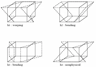
Figure 3.Hourglass modes in x-direction for a one-point quadrature hexahedron
Unlike the one-point quadrature hexahedron (Belytschko et al., 1993) comprising twelve hourglass modes given by Figure 3, only six hourglass modes are found for the SHB8PS element. They are composed of h3 and h4 vectors as expressed in Equation [21] and illustrated in Figure 4 below:
2.4. Stabilization and hourglass control
The control of the six hourglass modes of the SHB8PS element, as revealed by Equation [21], is achieved by adding a stabilization stiffness to the stiffness matrix
e
K . This part is drawn from the approach of (Belytschko et al., 1993), who applied an efficient stabilization technique together with an assumed strain method for the eight-node hexahedral element with uniform reduced integration. The stabilization forces are deduced in the same way. It is important to note that this stabilization part is treated completely independently from the assumed strain projection part, the later being intended to eliminate the locking phenomena. This projection technique will be applied in Section 2.5.
The starting point consists of decomposing the discrete gradient operator B into two parts as follows:
12 34
B=B +B [22]
The first term in this additive decomposition is given by Equation [18]. The second term B34 is precisely the one that vanishes at the Gauss points. It is given by the following matrix form:
4 , 3 4 , 3 4 , 3 4 4 34 , , 3 3 4 , , 3,4 3 4 , , 3 3,4 0 0 0 0 0 0 0 0 0 T x T y T z T T y x T T z y T T z x h h h B h h h h h h α α α α α α α α α α α α α α α α α α α α α α α α α α α
γ
γ
γ
γ
γ
γ
γ
γ
γ
= = = = = = = = = =
∑
∑
∑
∑
∑
∑
∑
∑
∑
[23]In the standard displacement approach, the stiffness and internal forces are defined as: e e int T e T f K B C B d B
σ
d Ω Ω = = ⋅ ⋅ Ω ⋅ Ω∫
∫
[24]By introducing the additive decomposition [22] of the B matrix, the stiffness matrix becomes: 12 12 12 34 34 12 34 34 e e e e T T e T T K B C B d B C B d B C B d B C B d Ω Ω Ω Ω = ⋅ ⋅ Ω + ⋅ ⋅ Ω + ⋅ ⋅ Ω + ⋅ ⋅ Ω
∫
∫
∫
∫
[25]which can be simply written as:
12
e STAB
K =K +K [26]
The first term, K12, is the only one taken into account when the stiffness is
evaluated at the Gauss points as defined above. It reads:
5 12 12 12 12 12 1 ( ) ( ) ( ) ( ) e T T I I I I I K B C B d
ω ζ
Jζ
Bζ
C Bζ
= Ω =∫
⋅ ⋅ Ω=
∑
⋅ ⋅ [27]The second term, KSTAB, represents the stabilization stiffness since it vanishes if
evaluated at the Gauss points:
12 34 34 12 34 34 e e e T T T STAB K B C B d B C B d B C B d Ω Ω Ω =
∫
⋅ ⋅ Ω +∫
⋅ ⋅ Ω +∫
⋅ ⋅ Ω [28]In a similar way, the internal forces of the element can be written as:
12
STAB
int int
f = f + f [29]
The first term, f12int, is the only one taken into account when the forces are evaluated at the Gauss points:
5 12 1 12 ( ) ( ) 12( ) ( ) e I I I I I T T int f B
σ
dω ζ
Jζ
Bζ σ ζ
= Ω =∫
⋅ Ω =∑
⋅ [30]The second term fSTAB of Equation [29] represents the stabilization forces and should be consistently calculated according to the stabilization stiffness given by Equation [28].
Since the stabilization stiffness and forces cannot be calculated properly at the integration points, we will calculate them in the co-rotational coordinate system proposed by (Belytschko et al., 1993), in order to prevent the hourglass mode phenomena. An intermediate stage for this approach consists of projecting B onto a
B matrix, in order to eliminate the remaining locking problems.
2.5. Assumed strain field and orthogonal projection
The discrete gradient operator is projected onto an appropriate sub-space in order to eliminate shear and membrane locking. This projection technique can be derived from the formalism of the assumed strain method. It is also shown that this approach can be justified within the framework of the Hu-Washizu nonlinear mixed variational principle (see for instance Korelec et al., 1996). Indeed, this three-field variational principle reads:
(
)
( , , ) ( ) 0 e e T T T ext s v d v d d fδπ
ε σ
δε σ
δ σ
ε
δ
Ω Ω =∫
⋅ Ω +∫
⋅ ∇ − Ω − & ⋅ =& & & [31]
where
δ
denotes a variation, v the velocity field,ε
& the assumed strain rate,σ
the interpolated stress,σ
the stress evaluated by the constitutive law, d& the nodal velocities, fext the external nodal forces and ∇s( )v the symmetric part of the velocity gradient. The assumed strain formulation used to construct the SHB8PS element is a simplified form of the Hu-Washizu variational principle as described by (Simo et al., 1986). In this simplified form, the interpolated stress is chosen to be orthogonal to the difference between the symmetric part of the velocity gradient and the assumed strain rate. Consequently, the second term of Equation [31] vanishes and one obtains:( , ) 0 e T T ext v d d f
δπ
ε
δε σ
δ
Ω =∫
⋅ Ω − & ⋅ = & & [32]In this form, the variational principle is independent of the stress interpolation, since the interpolated stress is eliminated and does not need to be defined. The discrete equations then only require the interpolation of the velocity and of the assumed strain field. The assumed strain rate ε& is expressed in terms of a B matrix, projected starting from the classical discrete gradient B defined by Equations [14] and [15]:
( , )x t B x d t( ) ( )
ε
& = ⋅ & [33]Once this expression replaced in the variational principle [32], the new expressions for the elastic stiffness and internal forces are obtained:
, ( ) e e T int T e K B C B d f B
σ ε
d Ω Ω =∫
⋅ ⋅ Ω =∫
⋅ & Ω [34]Before defining the projected B operator, let us replace in the previous equations the Hallquist form of the bi vectors (Equation [9]) by the mean form bˆi
from (Flanagan-Belytschko, 1981): , 1 ˆ ( , , ) , 1, 2, 3 e e T i i
b N ξ η ζ d i Mean value form
Ω
Ω
=
∫
Ω = [35]Accordingly, the vectors
γ
α are replaced by the vectorsγ
ˆα defined as:3 1 ˆ ˆ
1
8
( T ) j j j h h x b α α αγ
= =
− ⋅
∑
[36]Finally, the B matrix, defined by Equation [15], is replaced by the ˆB operator defined by: , , , , , , , , , ˆ ˆ 0 0 ˆ ˆ 0 0 ˆ ˆ 0 0 ˆ ˆ ˆ ˆ ˆ 0 ˆ ˆ ˆ ˆ 0 ˆ ˆ 0 ˆ ˆ T T x x T T y y T T z z T T T T y y x x T T T T z z y y T T T T z z x x b h b h b h B b h b h b h b h b h b h α α α α α α α α α α α α α α α α α α
γ
γ
γ
γ
γ
γ
γ
γ
γ
+ + + = + + + + + +
[37]The approach developed earlier still applies, as well as the expressions of the stabilization stiffness and internal forces, if the same additive decomposition is adopted:
12 34
ˆ ˆ ˆ
It is noteworthy that in the former version of the SHB8PS element, the Hallquist forms bi have been replaced with the mean expressions bˆi of Flanagan-Belytschko only in the stabilization terms
34
ˆB and thus KSTAB.
It is also important to note that the two forms bi and bˆi have been tested on a large number of test problems and that Flanagan-Belytschko’s mean form performed better in all cases. Its better convergence is even more dramatic when a few, highly distorted elements are used. Similar results have been found by (Belytschko et al., 1993) with an assumed strain, eight-node solid element with one-point quadrature.
At this stage, one can project the ˆB operator from Equation [38] onto a ˆB operator such as:
12 34
ˆ ˆ ˆ
B =B +B [39]
It is clear that only the second term ˆB34 from Equation [38] is projected; the first term ˆB12 remains unchanged and is given by Equation [18] where the vectors bi are replaced by bˆi . The operator ˆB34 is projected onto ˆB34 given by:
4 , 3 4 , 3 3, 3 34 4, 4 ˆ 0 0 ˆ 0 0 ˆ 0 0 ˆ 0 0 0 0 0 0 ˆ 0 0 T x T y T z T x h h h B h α α α α α α
γ
γ
γ
γ
= = =
∑
∑
[40]The elastic stiffness is then given by Equation [26] as the sum of the following two contributions: 5 12 12 12 12 12 1 ˆ ˆ ( ) ( )ˆ ( ) ˆ ( ) e T T I I I I I K B C B d
ω ζ
Jζ
Bζ
C Bζ
= Ω =∫
⋅ ⋅ Ω=
∑
⋅ ⋅ [41] 12 34 34 12 34 34 ˆ ˆ ˆ ˆ ˆ ˆ e e e T T T STAB K B C B d B C B d B C B d Ω Ω Ω =∫
⋅ ⋅ Ω +∫
⋅ ⋅ Ω +∫
⋅ ⋅ Ω [42]The stabilization stiffness, Equation [42], is calculated in a co-rotational coordinate system (Belytschko et al., 1993). This orthogonal co-rotational system that is embedded in the element and rotates with the element is chosen to be aligned with the referential coordinate system (see Figure 5). This choice is justified here by the rotation extracted from the polar decomposition of the transformation gradient (Abed-Meraim et al., 2001, 2002). As noticed by (Belytschko et al., 1993), such a co-rotational approach has numerous advantages: simplified expressions for the above stabilization stiffness matrix, whose first two terms vanish; more effective treatment of the shear locking in this frame; the co-rotational system assures a frame-invariant element.
Figure 5. Schematic representation of the co-rotational coordinate system
The main equations defining the chosen co-rotational coordinate system are given hereafter. First, the components of the column vectors forming the rotation matrix are computed:
1 1 , 2 2 , 1, 2, 3 T T i i i i a = Λ ⋅x a = Λ ⋅x i= [43] with: 1 2 3 ( 1,1,1, 1, 1,1,1, 1) ( 1, 1,1,1, 1, 1,1,1) ( 1, 1, 1, 1,1,1,1,1) T T T Λ = − − − − Λ = − − − − Λ = − − − −
[44]Then, the correction term ac is calculated so that the orthogonality relation
(
)
1 2 0 T c a ⋅ a +a = is verified: 1 2 1 1 1 T c T a a a a a a ⋅ = − ⋅ [45]The third base vector
a
3 is then obtained by the cross-product:(
)
3 1^ 2 c
a =a a +a [46]
The rotation matrix R that maps a vector in the global coordinate system to the co-rotational system is finally given, after normalization, by:
1 2 3 1 2 3 1 2 3 , , , 1, 2,3 i i ci i i i i c a a a a R R R i a a a a + = = = = + [47]
The stabilization terms (stabilization stiffness and internal forces, Equation [42]) are computed in this co-rotational coordinate system, where several terms simplify. Indeed, in this co-rotational system one obtains:
( )
( )
( )
(
(
)(
)
)
, 2 2 2 , , 4, , , 1 3 1 3 0 3 e e e e e i j T T j j k k j i k i i T i i T i j j i k k ii ij h d x x h d h d h d x h h d x H H Ω Ω Ω Ω Ω Ω = Λ ⋅ Λ ⋅ = Ω = Ω = Ω = Λ ⋅ = Ω = Λ ⋅
∫
∫
∫
∫
∫
[48]In these last formulas, there is no sum on repeated subscripts. Moreover, subscripts
i j
,
and k in the expressions of Hii and Hij are two by two distinct and take the values 1, 2 and 3 with all of the possible permutations. Using these explicit expressions, the stabilization stiffness given in Equation [42] is obtained completely analytically in this co-rotational system as:11 12 13 21 22 23 31 32 33 STAB
k
k
k
K
k
k
k
k
k
k
=
[49]where the 8 x 8 matrices kij are given by: 11 22 11 11 3 3 4 4 22 3 3 4 4 33 4 4 1 3 1 3 ( 2 ) ( 2 ) 1 3 0 ,
ˆ ˆ
ˆ ˆ
ˆ ˆ
ˆ ˆ
ˆ ˆ
T T T T T ij k H k H k H k i jλ
µ
λ
µ
µ
γ γ
γ γ
γ γ
γ γ
γ γ
= + = + = = ≠
+
+
[50]Note that an improved, plane-stress type constitutive law is adopted for the SHB8PS element. This specific law is given by:
2 2 0 0 0 0 2 0 0 0 0 0 0 0 0 0 0 0 0 0 0 0 0 0 0 0 0 0 0 0 0 2(1 ) 1 E C E E λ µ λ λ λ µ µ µ µ ν µ λ ν ν + + = = = + −
[51]On one hand, the choice of this constitutive matrix avoids locking encountered with a full three-dimensional law and, on the other hand, allows the deformation energy associated to the strains normal to the mean surface of the element to be taken into account.
For the computation of the internal forces of the element, the same approach is adopted (Abed-Meraim et al., 2001, 2002). The additive decomposition [39] and the projection [40] allow the calculation of the stabilization forces:
5 1 12 ˆ ( ) ( ) ( ) ( ) STAB I I I I I T int f
ω ζ
Jζ
Bζ σ ζ
f = =∑
⋅ + [52] where: 1 2 3 STAB STAB STAB STAB f f f f
=
[53]4 3
ˆ ,
1, 2,3
STAB i i fQ
α αi
α=γ
=
∑
=
[54]The Qiα, called generalized stresses and entering the expressions of the stabilization forces, are related to the so-called generalized strains qiα by the following incremental equations:
13 11 13 14 11 14 23 22 23 24 22 24 33 34 11 34 1 3 1 3 1 3 ( 2 ) ( 2 ) ( 2 ) ( 2 ) 0 Q H q Q H q Q H q Q H q Q Q H q
λ
µ
λ
µ
λ
µ
λ
µ
µ
= + = + = + = + = =
& & & & & & & & & & & [55]The generalized strain rates q&iα are given by:
=3, 4
ˆ
T,
1, 2,3 ,
i i
q
&
α=
γ
α⋅
d
&
i
=
α
[56] The previous expressions for the stabilization stiffness and forces hold for an elastic behavior. In the case of elastic-plastic behavior, the Young’s modulusE
is replaced by the mean tangent modulus (i.e. the average of the tangent moduli at the five Gauss points across the thickness). This choice avoids the too stiff response corresponding to a purely elastic hourglass stabilization. Thus this leads to an adaptive element provided with a stabilization that automatically adjusts to the physical situation of the element: elastic or elastic-plastic.3. Numerical results
In order to validate the new version of the SHB8PS element, its performances have been tested, based on the analysis of a variety of benchmark problems frequently used in the literature (namely a large number of numerical tests). For each test problem, the results were compared to the reference solutions and, on the other hand, to those given by the previous version of the SHB8PS element (Legay et al., 2003). Note that several projections have been formulated in this study and extensively tested over a wide range of benchmark problems. The retained projection
that is presented here is the one that showed the best convergence and exhibited no transverse shear and membrane locking phenomena. This projection improved the former version of the SHB8PS element in all cases and especially in the test of the pinched hemispherical shell where the improvement is significant. The results given hereafter concern this test case, as well as a set of representative popular benchmark problems commonly used to test finite element perfomances.
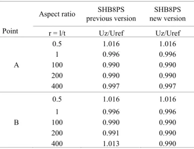
3.1. Admissible aspect ratios for the element
This linear benchmark problem was used to evaluate the aspect ratio limit of the previous version of the SHB8PS element (Legay et al., 2003). It is also suitable for testing the behavior of the element when non structured, irregular meshes are employed as well as for analyzing locking phenomena in the limit of high aspect ratios. In Figure 6, the cantilever beam geometry is shown and regular as well as irregular mesh data are specified.
Figure 6.Cantilever beam: regular and irregular mesh specification
The length and the width of the beam are fixed: L=100, l=10; while the thickness t is a varying parameter. The elastic properties are E=6.825×10⁷ and ν=0.3. A
bending load, P=4, is applied at the free end of the beam and the results are compared with the analytical solutions given by beam theory.
Table 2. Normalized displacements at points A and B for regular mesh
Aspect ratio previous version SHB8PS new version SHB8PS
Point r = l/t Uz/Uref Uz/Uref
0.5 1.016 1.016 1 0.996 0.996 A 100 0.990 0.990 200 0.990 0.990 400 0.997 0.997 0.5 1.016 1.016 1 0.996 0.996 B 100 0.990 0.990 200 0.991 0.990 400 1.013 0.990
Table 3.Normalized displacements at points A and B for irregular mesh
Aspect ratio previous version SHB8PS new version SHB8PS Point r = l/t Uz/Uref Uz/Uref
0.5 0.984 0.984 1 0.965 0.965 A 100 0.958 0.958 200 0.957 0.958 400 0.980 0.980 0.5 0.973 0.973 1 0.953 0.953 B 100 0.947 0.947 200 0.946 0.946 400 0.966 0.967
A fixed mesh with 10 elements and a single element through the thickness is used in both regular and irregular mesh. For regular mesh, each element is a 10×10 square: l is the side of the square and r l t= is the varying aspect ratio. The same aspect ratio definition is adopted for the irregular mesh (see Figure 6). The normalized vertical displacements at points A and B for different aspect ratios are
reported in Table 2, for regular mesh, and in Table 3 for irregular mesh. In this cantilever beam test, we can observe that the quality of the results declines once the aspect ratio exceeds 400 for regular mesh as well as for irregular mesh. Moreover, the in-plane distortion of the elements does not affect significantly the accuracy of the results. However, we can notice that this mesh distortion leads to a slightly stiffer stiffness than when regular mesh is used.
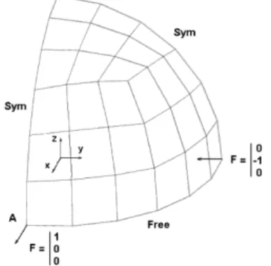
3.2. Pinched hemispherical shell
This test problem has become very popular and it has been used by many authors since (MacNeal et al., 1985). It is very severe since the transverse shear and membrane locking phenomena are very important and emphasized by the problem geometry (distorted, skewed elements). This problem was studied in detail by (Belytschko et al., 1989) who showed that, since all the elements are incurved, the intensity of the membrane and shear locking is increased. They also showed that in this doubly-curved shell problem the membrane locking is much more severe than the shear locking. Figure 7 shows the geometry, loading and boundary conditions for this problem. The radius is R=10, the thickness is t=0.04, the Young’s modulus is E=6.825×10⁷ and the Poisson’s ratio is ν =0.3. Using the symmetry of the problem
(i.e. planes (XZ) and (YZ)), only a quarter of the hemisphere is meshed using a single
element through the thickness and with two unit loads along directions Ox and Oy. Except for the symmetry, the boundary conditions are free; nevertheless, the displacement of one point in the z-direction is fixed in order to prevent rigid body motions. According to the reference solution (MacNeal et al., 1985), the displacement of point A along the x-direction equals 0.0924 (see Figure 7).
Figure 7.Geometry and loading of the pinched hemispherical shell problem
The convergence results are reported in Table 4 in terms of the normalized displacement at point A in the x-direction. The new version of the SHB8PS element is compared to the former one and to the three elements HEX8, HEXDS and H8-ct-cp.
The HEX8 element is the standard, eight-node, full integration solid element (eight Gauss points). The HEXDS element is an eight-node, four-point quadrature solid element (Liu et al., 1998). The H8-ct-cp element is presented in the PhD thesis of Lemosse (Lemosse, 2000). Table 4 shows that the new version of the SHB8PS element provides an excellent convergence and shows no locking.
Table 4.Normalized displacement at point A of the pinched hemispherical shell
SHB8PS previous
version HEX8 HEXDS H8-ct-cp SHB8PS new version Number of
elements Ux/Uref Ux/Uref Ux/Uref Ux/Uref Ux/Uref
12 0.0629 0.0005 0.05 0.8645 27 0.0474 0.0011 1.0155 48 0.1660 0.0023 0.408 0.35 1.0098 75 0.2252 0.0030 0.512 0.58 1.0096 192 0.6332 0.0076 0.701 0.95 1.0008 363 0.8592 0.0140 0.800 1.0006 768 0.9651 0.0287 1.0006 1462 0.9910 0.0520 1.0009
3.3. Twisted cantilever beam
This test has been introduced by (MacNeal et al., 1985) and has been extensively used to test the elements performance due to the use of warped configuration. It is considered now as a reference shell test (see Batoz et al., 1992). The geometry is twisted by an angle of 90° between the two ends of the beam. This distorts the elements and thus increases the severity of the test.
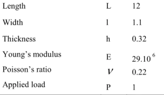
Figure 8 shows the geometry of the twisted beam, the boundary conditions and the two types of applied loads. The left-side end of the beam is fixed and a unit shear load P=1 is applied at its right-side end. Two load directions are studied: P1 (unit in-plane load) and P2 (unit out-of-in-plane load). The geometric and material parameters for this problem are listed in Table 5.
Figure 8.Geometry and loading cases of the twisted cantilever beam
Table 5.Geometric and material parameters of the twisted cantilever beam
Length L 12 Width l 1.1 Thickness h 0.32 Young’s modulus E 29.106 Poisson’s ratio
ν
0.22 Applied load P 1 3.3.1. In-plane loading (P1)In this first case, the unit load is applied in the plane of the beam along the vertical z-direction (see Figure 8). The analytical tip displacements in the loading directions are given in (MacNeal et al., 1985). For the loading case P1, the displacement at point A in the loading direction Oz (see Figure 8) should be equal to 5.424×10⁻³.
Table 6 shows the results for this test in terms of convergence with the refinement of the mesh. The normalized displacement at point A in the loading direction Oz is reported for three elements, with different mesh densities and only one element through the thickness. The new SHB8PS element is compared to its previous version and to the HEX8 element. The later represents the standard, eight-node linear solid element with full integration (eight Gauss points). Both versions of the SHB8PS element provide excellent accuracy and converge very rapidly (four elements are enough), while the HEX8 element exhibits numerical locking and thus a much slower convergence.
Table 6. Normalized displacement in the z-direction at point A of the twisted cantilever beam HEX8 SHB8PS previous version SHB8PS new version Number of elements
Uz/Uref Uz/Uref Uz/Uref 2x1x1=2 0.008 1.035 1.041 4x1x1=4 0.031 0.995 1.014 12x2x1=24 0.206 0.997 0.999 24x4x1=96 0.490 0.998 0.999
3.3.2. Out-of-plane loading (P2)
This second, out-of-plane loading case consists of a horizontal unit load P=1 in the y-direction (see Figure 8). The reference solution is also given by (MacNeal et al., 1985). For this P2 loading, the displacement at point A in the loading direction (see Figure 8) should be equal to 1.754×10⁻³.
Table 7.Normalized displacement in the y-direction at point A of the twisted beam
HEX8 SHB8PS previous version SHB8PS new version Number of elements
Uy/Uref Uy/Uref Uy/Uref 2x1x1=2 0.023 0.705 0.867 4x1x1=4 0.081 0.906 0.952 12x2x1=24 0.333 0.986 0.994 24x4x1=96 0.592 0.996 0.998
Table 7 shows the convergence results for this case in terms of the normalized displacement at point A in the loading direction Oy. The same three elements are compared. Again, the two versions of the SHB8PS element exhibit a fast convergence (starting from about ten elements), while the HEX8 element shows locking and slow convergence. Note that the new version of the SHB8PS element shows better performance for coarse meshes. For this out-of-plane loading case, the coarse meshes involving only two and four elements give less accurate results as compared to the previous in-plane loading case (vertical load). This can be understood by analyzing the orientation of the Gauss points (Figure 9). Indeed, at the fixed end where the maximum bending moment is localized, there is a single Gauss point in the load direction P2 while there are five in the direction of load P1.
Figure 9.Position of the Gauss points in the mesh of the twisted cantilever beam
Two other versions of this twisted beam problem can be found in the literature (Simo et al., 1989), (Batoz et al., 1992). These versions differ only by their lower thickness: 0.05 and 0.0032, which allows us to evaluate the effects of locking phenomena in the limit of high aspect ratios. The reference results for different thicknesses are summarised in Table 8 below.
Table 8.Reference solution for the twisted beam test and different thickness values
Thickness In-plane loading Out-of-plane loading h=0.32 5.424×10⁻³ 1.754×10⁻³
h=0.05 1.39 0.3431
h=0.0032 5.316×10+3 1.216×10+3
The normalized displacements for a 24×2×1 mesh in both in-plane and out-of-plane loading conditions are reported in Table 9 for the three different thicknesses.
Table 9.Normalized results for the twisted beam test and different thickness values
Thickness In-plane loading Out-of-plane loading
h=0.32 0.999 0.998
h=0.05 0.998 0.995
Similar results as in the first benchmark problem of a cantilever beam with extreme aspect ratios are found. Indeed, we can observe that the accuracy of the results is not affected by the high aspect ratio. In the case of the lowest thickness (h=0.0032) the aspect ratio value is about 150, which confirms the good behavior of the SHB8PS element even when very thin shell problems are considered.
3.4. Pinched cylinder with end diaphragms
A cylindrical shell loaded by a pair of concentrated vertical forces at its middle section is considered here. Both ends of the cylinder are covered with rigid diaphragms that allow displacement only in the axial direction (see Figure 10). This test has been treated by many authors, among them (Belytschko et al., 1989) and (Chen et al., 2004). It is considered as a selective test problem since they have shown that shear locking is more severe than membrane locking. The geometric and material parameters for this problem are reported in Table 10.
Figure 10.Geometry, boundary conditions and loading for the pinched cylinder
Owing to symmetry, only one eighth of the cylinder is modeled using 2×2, 4×4, 8×8, 16×16 and 32×32 meshes as illustrated in Figure 10.
Table 10.Geometric and material parameters of the pinched cylinder problem
Length L 600 Radius R 300 Thickness t 3 Young’s modulus E 3.106 Poisson’s ratio
ν
0.3 Applied load P 1The displacement at the loaded point in the loading direction is normalized with respect to the reference solution of 0.18248×10⁻⁴ and reported in Table 11.
Table 11.Normalized displacements at the loaded point of the pinched cylinder
SHB8PS previous version SHB8PS new version Mesh layout Uz/Uref Uz/Uref 2x2 0.043 0.101 4x4 0.223 0.387 8x8 0.708 0.754 16x16 0.937 0.940 32x32 0.996 0.997
As we can see in Table 11, the new version of the SHB8PS element performs better than the former one, especially for coarse meshes.
3.5. Simply supported circular plate under uniform load
The aim of this test problem is to investigate the effect of low thickness values (i.e. high aspect ratios) on the convergence of the SHB8PS element. This test was extensively used in the finite element technology of shell and plate elements, since an affected convergence may reveal some locking problems. Four different meshes composed of 12, 27, 48 and 75 elements are used as illustrated in Figure 11.
The coordinates of points O, A, B, C, D, E and F as shown in Figure 11 are given in Table 12 below:
Table 12.Coordinates of points O, A, B, C, D, E and F of the quarter of the plate
O A B C D E F
x 0. 1. 2 2 0. 0.5 0. 0.4
y 0. 0. 2 2 1. 0. 0.5 0.4 z 0. 0. 0. 0. 0. 0. 0.
Table 13.Normalized deflections of the uniformly loaded circular plate
Thickness value Point Mesh t=0.1 t=0.01 t=0.001 12 0.943 0.944 0.944 27 0.975 0.976 0.975 O 48 0.985 0.986 0.986 75 0.990 0.991 0.991 12 0.920 0.920 0.920 27 0.965 0.964 0.964 D 48 0.979 0.979 0.979 75 0.987 0.987 0.987 12 0.920 0.920 0.920 27 0.965 0.964 0.964 E 48 0.979 0.979 0.979 75 0.987 0.987 0.987 12 0.910 0.910 0.910 27 0.961 0.960 0.960 F 48 0.977 0.977 0.977 75 0.985 0.985 0.985
Different radius to thickness ratios have been considered, namely thick plate (R/t=10), thin plate (R/t=100) and very thin plate (R/t=1000), respectively. The reference solutions are based on classical Kirchhoff theory for thin plates, or
Reissner-Mindlin theory for thick plates as quoted in (Timoshenko et al., 1959) and (Jirousek et al., 1995). The normalized deflections at points O, D, E and F are reported in Table 13 for different meshes and radius to thickness ratios, R/t.
As we can see in Table 13, the SHB8PS shows good convergence in all cases and no shear locking appears for the thinnest plate with R/t=1000. Note that for the thinnest plate, the aspect ratio varies from about 250 for the 12-element mesh to about 100 for the 75-element mesh.
3.6. Uniformly loaded square plate with simple support
Similar convergence studies are carried out on square plates under uniform load. The plate is simply supported and owing to symmetry, only one quarter of the plate is modeled and divided into a mesh of N×N elements as shown in Figure 12. Young’s modulus and Poisson’s ratio are taken equal to 1 and 0.3, respectively. The convergence tests for the plate are evaluated using three different L/t ratios of 10, 100 and 1000 corresponding to thick, thin and very thin plates, respectively.
The reference solutions for thin plates are based on Kirchhoff theory as quoted in (Timoshenko et al., 1959); for thick plates, they are taken from (Jirousek et al., 1995). Table 14 summarizes the normalized results for the central deflection with different meshes and span to thickness ratios, L/t. Similarly to the preceding test of uniformly loaded circular plates, we can observe that the SHB8PS element performs well in this test problem and shows quite a good convergence for both thick and thin plate situations. Even for a very thin plate, L/t=1000, where the aspect ratio is equal to 250 for the mesh with 2×2 elements, the convergence has proven to be insensitive to high aspect ratios, which confirms that the element does not suffer from shear locking.
Table 14.Normalized central deflection of the uniformly loaded square plate
Span to thickness ratio Mesh L/t=10 L/t=100 L/t=1000 2×2 0.986 1.075 1.073 4×4 1.000 1.018 1.019 8×8 1.004 1.008 1.004 16×16 1.004 1.008 1.002
4. Discussion and conclusions
A new formulation of the solid-shell element SHB8PS has been performed and implemented into the implicit, nonlinear finite element code Stanlax-INCA. This new version has been evaluated, based on a variety of a large number of popular benchmark problems frequently used in the literature. Let us recall that this solid-shell element is based on a purely three-dimensional formulation (eight-node hexahedron and only three translational degrees of freedom per node). A reduced integration is used to improve the computational efficiency and an effective stabilization is built for hourglass mode control. Five integration points are used along a particular chosen direction designated as the “thickness”, allowing for accurate modeling of bending-dominated structural problems using only a single element through the thickness. Moreover, the projection adopted in this new version of the element much better eliminates the various numerical locking phenomena. Indeed, the excellent efficiency and convergence properties of the element have been clearly demonstrated through numerous tests. All these tests show that there is no residual locking (membrane, shear). In particular, the improvement is significant in the pinched hemispherical shell problem, where the amount of locking observed in the former version has been eliminated. The validation of this element through nonlinear applications, including elastic-plastic buckling problems and large displacement and rotation simulations, is currently performed. Also, a new explicit version of this element will be implemented into an explicit dynamic code for impact and crash analyses.
5. References
Abed-Meraim F., Combescure A., Stabilité des éléments finis sous-intégrés, Rapport interne n° 247, LMT de Cachan, janvier 2001.
Abed-Meraim F., Combescure A., “SHB8PS a new intelligent assumed strain continuum mechanics shell element for impact analysis on a rotating body”, First M.I.T. Conference
Abed-Meraim F., Combescure A., “SHB8PS – a new adaptative, assumed-strain continuum mechanics shell element for impact analysis”, Computers & Structures, vol. 80, 2002, p. 791-803.
Ahmad S., “Analysis of thick and thin shell structures by curved finite elements”,
International Journal for Numerical Methods and Engineering, vol. 2, 1970, p. 419-451. Alves de Sousa R.J., Cardoso R.P.R., Fontes Valente R.A., Yoon J.W., Gracio J.J.,
Natal Jorge R.M., “A new one-point quadrature enhanced assumed strain (EAS) solid-shell element with multiple integration points along thickness: Part I – Geometrically linear applications”, International Journal for Numerical Methods and Engineering, vol. 62, 2005, p. 952-977.
Alves de Sousa R.J., Cardoso R.P.R., Fontes Valente R.A., Yoon J.W., Gracio J.J., Natal Jorge R.M., “A new one-point quadrature enhanced assumed strain (EAS) solid-shell element with multiple integration points along thickness: Part II – Nonlinear applications”, International Journal for Numerical Methods and Engineering, vol. 67, 2006, p. 160-188.
Alves de Sousa R.J., Yoon J.W., Cardoso R.P.R., Fontes Valente R.A., Gracio J.J., “On the use of a reduced enhanced solid-shell (RESS) element for sheet forming simulations”,
International Journal of Plasticity, vol. 23, 2007, p. 490-515.
Ayad R., Batoz J.L., Dhatt G., « Un élément quadrangulaire de plaque basé sur une formulation mixte-hybride avec projection en cisaillement », Revue européenne des
éléments finis, vol. 4, 1995, p. 415-440.
Ayad R., Dhatt G., Batoz J.L., “A new hybrid-mixed variational approach for Reissner-Mindlin plates: The MiSP model”, International Journal for Numerical Methods and
Engineering, vol. 42, 1998, p. 1149-1179.
Bathe K.-J., Dvorkin E.N., “Four-node plate bending element based on Mindlin/Reissner plate theory and a mixed interpolation”, International Journal for Numerical Methods
and Engineering, vol. 21, 1985, p. 367-383.
Bathe K.-J., Dvorkin E.N., “Formulation of general shell elements – The use of mixed interpolation of tensorial components”, International Journal for Numerical Methods and
Engineering, vol. 22, 1986, p. 697-722.
Batoz J.L., Dhatt G., Modelling of structures by finite elements, Hermès, Paris, 1992. Belytschko T., Ong J.S.-J., Liu W.K., Kennedy J.M., “Hourglass control in linear and
nonlinear problems”, Computer Methods in Applied Mechanics and Engineering, vol. 43, 1984, p. 251-276.
Belytschko T., Wong B.L., Stolarski H., “Assumed strain stabilization procedure for the 9-node Lagrange shell element”, International Journal for Numerical Methods and
Engineering, vol. 28, 1989, p. 385-414.
Belytschko T., Bindeman L.P., “Assumed strain stabilization of the eight node hexahedral element”, Computer Methods in Applied Mechanics and Engineering, vol. 105, 1993, p. 225-260.

![Figure 2. Reference space ( ξ η ζ , , ) and physical space ( x x x 1 , , 2 3 ) of the element Combining Equations [1], [2] and [4] leads to the expansion of the displacement field as a constant term, linear terms in x i and some terms depending on](https://thumb-eu.123doks.com/thumbv2/123doknet/7300660.209100/8.892.258.640.224.391/reference-physical-combining-equations-expansion-displacement-constant-depending.webp)