HAL Id: hal-01796066
https://hal.archives-ouvertes.fr/hal-01796066
Submitted on 19 May 2018
HAL is a multi-disciplinary open access
archive for the deposit and dissemination of
sci-entific research documents, whether they are
pub-lished or not. The documents may come from
teaching and research institutions in France or
L’archive ouverte pluridisciplinaire HAL, est
destinée au dépôt et à la diffusion de documents
scientifiques de niveau recherche, publiés ou non,
émanant des établissements d’enseignement et de
recherche français ou étrangers, des laboratoires
Workspace, Joint space and Singularities of a family of
Delta-Like Robot
Ranjan Jha, Damien Chablat, Luc Baron, Fabrice Rouillier, Guillaume Moroz
To cite this version:
Ranjan Jha, Damien Chablat, Luc Baron, Fabrice Rouillier, Guillaume Moroz. Workspace, Joint
space and Singularities of a family of Delta-Like Robot. Mechanism and Machine Theory, Elsevier,
2018, 127, pp.73-95. �10.1016/j.mechmachtheory.2018.05.004�. �hal-01796066�
Workspace, Joint space and Singularities of a family of
Delta-Like Robot
Ranjan Jhaa, Damien Chablatb,∗, Luc Baronc, Fabrice Rouillierd, Guillaume
Moroze
a
BioMedical Instrumentation Division, CSIR- Central Scientific Instruments Organisation, Chandigarh, India
bLaboratoire des Sciences du Num´erique de Nantes, UMR CNRS 6004, Nantes, France. c
Department of Mechanical Engineering, ´Ecole Polytechnique de Montr´eal, Qu´ebec, Canada
d
INRIA Paris-Rocquencourt, Institut de Math´ematiques de Jussieu, UMR CNRS 7586, Paris, France.
e
INRIA Nancy-Grand Est, Nancy, France.
Abstract
This paper presents the workspace, the joint space and the singularities of a family of delta-like parallel robots by using algebraic tools. The different func-tions of SIROPA library are introduced, which is used to induce an estimation about the complexity in representing the singularities in the workspace and the joint space. A Gr¨obner based elimination is used to compute the singularities of the manipulator and a Cylindrical Algebraic Decomposition algorithm is used to study the workspace and the joint space. From these algebraic objects, we propose some certified three-dimensional plotting describing the shape of works-pace and of the joint sworks-pace which will help the engineers or researchers to decide the most suited configuration of the manipulator they should use for a given task. Also, the different parameters associated with the complexity of the serial and parallel singularities are tabulated, which further enhance the selection of the different configuration of the manipulator by comparing the complexity of the singularity equations.
Keywords: Delta-like robot, Cylindrical algebraic decomposition, Workspace,
Gr¨obner basis, Parallel robot, Singularities
∗. Corresponding author
Email addresses: Ranjan.Jha@csio.res.in(Ranjan Jha), Damien.Chablat@cnrs.fr (Damien Chablat), Luc.Baron@polymtl.ca (Luc Baron), Fabrice.Rouillier@inria.fr (Fabrice Rouillier), Guillaume.Moroz@inria.fr (Guillaume Moroz)
Nomenclature
SIROPA Library for manipulator singularities analysis
CAD Cylindrical Algebraic Decomposition
IKP Inverse Kinematics problem
DKP Direct Kinematics problem
det Determinant of Jacobian matrix
R Revolute Joint
P Prismatic Joint
S Spherical Joint
ρ Actuated Joint Variables
X Pose Variables
A Direct parallel Jacobian matrices
B Inverse serial Jacobian matrices
1. Introduction
The workspace can be defined as the volume of space or the complete set of poses which the end-effector of the manipulator can reach. Many researchers 5
published several works on the problem of computing these complete sets for robot kinematics. Based on the early studies [1, 2], several methods for works-pace determination have been proposed, but many of them are applicable only to a particular class of robots. The workspace of parallel robots mainly depends on the actuated joint variables, the range of motion of the joints and the me-10
chanical interferences between the bodies of the mechanism. There are different techniques based on geometric [3, 4], discretization [5, 6, 7], and algebraic me-thods [8, 9, 10, 11, 12] which can be used to compute the workspace of parallel robot. The main advantage of the geometric approach is that it establishes the nature of the boundary of the workspace [13]. Also, it allows to compute the 15
surface and volume of the workspace while being very efficient in terms of sto-rage space, but when the rotational motion is included, it becomes less efficient. Interval analysis based methods can be used to compute the workspace but the computation time depends on the complexity of the robot and the requested accuracy [7]. Discretization methods are usually less complicated and can easily 20
take into account all kinematic constraints, but they require more space and computation time for higher resolutions. The majority of numerical methods used to determine the workspace of parallel manipulators includes the discreti-zation of the pose parameters for computing workspace boundaries [6]. There are other approaches, such that optimization algorithms [14] for fully serial or 25
parallel manipulators ; analytic methods for symmetrical spherical mechanisms [15]. In [16], a method for computing the workspace boundary for manipulators with a general structure is proposed, which uses a branch-and-prune technique to isolate a set of output singularities, and then classifies the points on such set according to whether they correspond to motion impediments in the works-30
pace. A Cylindrical Algebraic Decomposition (CAD) based method is used in [10, 17, 18] to model the workspace and joint space for the 3-RPS parallel ro-bot and delta-like roro-bots. The variations in the workspace, singularities, and joint space with respect to design parameter of a 3-RPS parallel manipulator is studied in [19].
Here, this paper presents the results obtained by applying algebraic methods for the workspace and joint space analysis of a family of a delta-like robot inclu-ding complexity information for representing the singularities in the workspace and the joint space. The CAD algorithm is used to study both the workspace and joint space, and a Gr¨obner based elimination process is used to compute the 40
parallel and serial singularities of the manipulator. The structure of the paper is as follows. Section 2 presents the mathematical tools and the introduction of SIROPA. Section 3 describes the architecture of the manipulator, including kinematic equation and joint constraints associated with the manipulators. Sec-tion 4 discusses the computaSec-tion of parallel as well as serial singularities and 45
their projections in workspace and joint-space. Section 5 and 6 present a compa-rative study on the shape of the workspace and joint space of different delta-like robots, respectively. Section 7 finally concludes the paper.
2. Algebraic Tools : SIROPA
SIROPA is a library for the MAPLE developed to analyze the singularities, 50
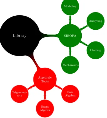
workspace and joint space of serial and parallel manipulators as well as tensegrity structures [20]. There are two main parts of the library shown in Fig.(1), the first one provides the algebraic tools to solve the constraint equations and convert the trigonometric equations in the algebraic form. The other one, SIROPA, provides modeling, analyzing and plotting functions for different manipulators, shown in 55
Fig.(2). Only a small part of these tools are used in the current paper.
Library SIROPA Modeling Analysing Plotting Mechanisms Algebraic Tools Base Algebra Extra Algebra Trigonome-tric
SIROPA
Modeling Analysing Plotting Mechanisms
CreateManipulator SubsPlus SubsParameters UnassignParameters ConstraintEquations SerialSingularities ParallelSingularities InfiniteEquations ParallelCuspidal SerialCuspidal Projection CellDecompositionPlus DVNumberOfSolutionsPlus auxDVNumberOfSolutionsPlus IsIntervalEmpty CellGraph PseudoSingularitiesDecomposition DirectInverseKinematics CellArea2D Plot2D PlotCurve3D Plot3D Plot3Dglsurf Plot3Dsurfex PlotWorkspace Configurations PlotRobot2D PlotRobot3D PlotCell3D PlotCell2D SetCellColors Trajectory ImageTrajectory Parallel 3RPR Parallel 3RPR full Parallel 3PRR ParallelPRP2PRR Parallel RPRRP Parallel RR RRR Parallel PRRP ParallelRPR2PRR Parallel3PPPS Serial3R Orthoglide Parallel3PRSd Parallel3PRSc F ig u r e 2 : L is t o f a ll th e d efi n ed fu n ct io n s in S IR O P A lib ra ry 4
2.1. Modeling Functions
SIROPA provides modeling functions such as CreateManipulator(), to vir-tually create the planar and spatial manipulators for further analysis. Below are the functions :
Functions
CreateManipulator Constructs a data structure of type Manipulator
SubsPlus Substitute coherently angles in a system
UnassignParameters Specify parameter values in a Manipulator
UnassignParameters Release parameters in a Manipulator
60
CreateManipulator
The function CreateManipulator() of SIROPA library in MAPLE soft-ware is used to virtually create the manipulator for analysis. Listing 1 shows the code architecture of the function.
65
As shown in Listing 1, compulsory inputs are identified as [c], while the optional ones as [o].Points,loops,chainsandactuators, are the input parame-ters to create the plot of the manipulator. The pose variables are the essential
input parameters to define the mechanism. The input parametersysis the set
of constraint equations associated with the motion of manipulator. 70 1 C r e a te M a n i p u l a t o r := p r o c ( 2 s y s[ c ] : : l i s t ({ a l g e b r a i c , a l g e b r a i c=a l g e b r a i c , a l g e b r a i c < a l g e b r a i c } ) 3 c a r t[ c ] : : l i s t ( name ) , 4 a r t i[ c ] : : l i s t ( name ) , 75 5 p a s s i v e[ o ] : : l i s t ( name ) , 6 geompars[ c ] : : l i s t ( name ) , 7 s p e c[ o ] : : { l i s t , s e t } ( name=a l g e b r a i c ) , 8 p l o t r a n g e[ o ] : : l i s t ( name=r a n g e ) , 9 p o i n t s[ p ] : : l i s t ( name= l i s t ( a l g e b r a i c ) ) , 80 10 l o o p s[ p ] : : l i s t ( l i s t ( name ) ) , 11 c h a i n s[ p ] : : l i s t ( l i s t ( name ) ) , 12 a c t u a t o r s[ p ] : : l i s t ({ l i s t ( name ) , name } ) ,
13 model[ o ] : : s t r i n g := ”No name ” ,
14 p r e c i s i o n[ o ] : : i n t e g e r := 4 , 85 15 { 16 n o r a d i c a l : : t r u e f a l s e := f a l s e 17 } 18 )
Listing 1: Architecture of Create Manipulator
Constructs a data structure of type Manipulator. 90
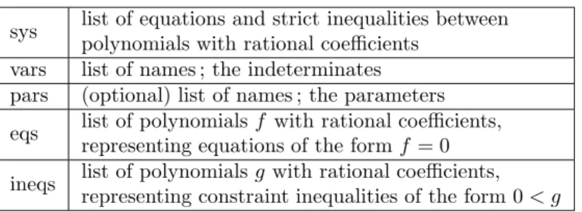
This function returns a data structure of type Manipulator containing the fields, briefly described below. Further, the values of these fields can be retrieved or changed according to the analysis to be performed.
Parameters
sys list of polynomials, polynomial equalities and polynomial
inequalities with rational coefficients : the implicit equa-tions and constraints of the considered manipulator
cart list of names : the pose variables
arti list of names : the control parameters ; default value : the
names ofsysnot invars
passive list of names : the passive variables ; default value : []
geompars list of names : the geometric parameters ; default value : the names ofsysnot incart, nor inarti
spec a list of equations of the form name=formula where name
is a parameter name and formula a polynomial with tri-gonometric function ; the new variables in a formula are handled in the same way as the replaced variable. default value : []
points list of name=list : the points of the robot with their co-ordinates ; default value : []
loops list of list of names : the frame loops of the robot default value : []
chains list of list of names : the frame chains of the robot default value : []
actuators list of names or list of names : the robot actuators ; a list of name is for a leg actuator, a name is for an angle actuator ; default value : []
model string : the name of the model ; default value : No name
precision an integer : the number of significative digits ; default va-lue : 4
Remarks
— Polynomials p appearing insys,Equations,GenericEquationsare
consi-95
dered implicitly as p=0.
— When a control parameter value is specified in spec, the parameter name
is removed from the ControlParemeters field. This is not the case for
the geometric parameters that appears in the fieldGeometricParameters
even if they are specified. 100
2.2. Analysing Functions
SIROPA provides the analysing function to compute the parallel and serial singularities. These functions are used to study both the workspace and joint space. The architecture of ConstraintEquations and CellDecompositionPlus are shown in Listing 2 and 3.
105 ConstraintEquations 1 C o n s t r a i n t E q u a t i o n s := p r o c ( r o b o t : : Manipulator , 2 { 3 c o n s t r a i n t s : : t r u e f a l s e := f a l s e 4 } 110
Returns
Equations a list of polynomials [p1, ..., pk] : the modeling
equations
Constraints a list of strict inequalities : the constraint inequa-lities
ArticularVariables a list of names : the control parameters
PassiveVariables a list of names : the remaining variables
GeometricParameters a list of names : the geometric parameters
GenericEquations a list of polynomials : the modeling equations with symbolic geometric parameters
GenericConstraints a list of strict inequalities : the constraint inequa-lities appearing in sys
Precision an integer : the number of correct digits
PoseValues the pose values substituted in the GenericEqua-tionsto get the Equations
ArticularValues the articular values substituted in the GenericE-quations to get the Equations
PassiveValues the passive values substituted in the GenericE-quations to get the Equations
GeometricValues the geometric values substituted in the Generi-cEquationsto get the Equations
DefaultPlotRanges ranges used by default for plotting if provided
Points the points coordinate of the robot
Loops the frame loops of the robot
Chains the frame chain of the robot
Actuators the actuators of the robot
Model a string : the name of the modeling
5 )
Listing 2: Architecture of ConstraintEquations function Computes the implicit equations induced by the constraints. Parameters
robot a data structure returned by a function mechanisms. Returns
115
A list of list of polynomials : each list represents a component of the equations satisfied by the constraints.
CellDecompositionPlus 1 C e l l D e c o m p o s i t i o n P l u s := p r o c ( equ : : l i s t ( a l g e b r a i c ) , 2 i n e q : : l i s t ( a l g e b r a i c ) , 120 3 v a r s : : l i s t ( name ) , 4 p a r s : : l i s t ( name ) := [ op ( i n d e t s ( [ equ , 5 i n e q ] , name ) minus { op ( v a r s ) } ) ] , 6 { 7 n o f a c t o r : : t r u e f a l s e := f a l s e , 125 8 g b f a c t o r : : t r u e f a l s e := f a l s e , 9 n o r e a l r o o t s t e s t : : t r u e f a l s e := f a l s e 10 }
Functions
ConstraintEquations Computes the implicit equations
indu-ced by the constraints.
SerialSingularities Computes the implicit equations
satis-fied by the singularities.
ParallelSingularities Computes the implicit equations
satis-fied by the singularities.
InfiniteEquations Computes the equations where the
ma-nipulator has infinitely many solutions.
ParallelCuspidal Computes the implicit equations
satis-fied by the cuspidal points.
SerialCuspidal Computes the implicit equations
satis-fied by the cuspidal points.
Projection Project on variables or expressions in a
polynomial system.
CellDecompositionPlus Describes the parameter space
accor-ding to the number of real roots.
NumberOfSolutionsPlus Returns the number of real solutions
of cells obtained by
CellDecomposition-Plus.
DVNumberOfSolutionsPlus Returns the number of real solutions on
the intersection points of the Discrimi-nant Variety.
auxDVNumberOfSolutionsPlus Auxiliary function Returns the
num-ber of real solutions on the intersection points of the Discriminant Variety.
IsIntervalEmpty Checks that a polynomial has no real
roots in an open interval.
CellGraph Computes the connexity graph of the
cells of a CAD.
DirectInverseKinematics Returns the cells having the same
an-tecedent.
CellArea2D Compute the area of the cells
retur-ned CellDecomposition or CellDecom-positionPlus.
CellLocationPlus Computes the cells of a decomposition
containing the given points.
11 )
Listing 3: Architecture of CellDecompositionPlus function Describes the parameter space according to the number of real roots. 130
Returns
A maple object : the same as the one returned by the maple function Root-Finding[Parametric][CellDecomposition]. The main difference is that it handles trigonometric expressions.
Parameters
equ a list of polynomials and trigonometric expressions : the
equations.
ineq a list of polynomials and trigonometric expressions : the
inequalities where each expression p stands for p>0.
vars a list of names : the variables of the system
pars a list of names : the parameters of the system ; default
value : the remaining variables ofequandineq
2.3. Plotting Functions
135
These functions are used to plot the workspace, joint space and singularity surfaces. Listing 4, 5, 6 and 7 shows the architecture of Plot2D, Plot3D, Configurations and PlotRobot3D, respectively.
Functions
Plot2D Plots a system of 2 variables
PlotCurve3D Plots a curve given by implicit equations in 3 variables
Plot3D Plots a system of 3 variables using maple internal
plot-ting functions
Plot3Dglsurf Plots a system of 3 variables using glsurf
Plot3Dsurfex Plots a system of 3 variables using surfex (software
based on surf)
PlotWorkspace Plot the border of a manipulator workspace
Configurations Computes the different possible positions
PlotRobot2D Plot a planar manipulator
PlotRobot3D Plot a 3D manipulator
PlotCell3D Plot the cells returned CellDecomposition or
CellDe-compositionPlus
PlotCell2D Plot the cells returned CellDecomposition or
CellDe-compositionPlus
SetCellColors Set colors to the numbers of solutions obtained by
NumberOfSolutionsPlus
Trajectory Display a given trajectory
ImageTrajectory Display a given trajectory
Plot2D 1 Plot2D := p r o c ( 140 2 s y s : : { a l g e b r a i c , e q u a t i o n ( a l g e b r a i c ) , l i s t ({ a l g e b r a i c , 3 e q u a t i o n ( a l g e b r a i c ) , a l g e b r a i c <a l g e b r a i c } ) , l i s t ( l i s t ({ 4 a l g e b r a i c , e q u a t i o n ( a l g e b r a i c ) , a l g e b r a i c <a l g e b r a i c } ) ) } , 5 e1 : : name = range , 6 e2 : : name = range , 145 7 { 8 p o i n t s : : t r u e f a l s e := f a l s e , 9 [ n o t e s t , d r a f t ] : : t r u e f a l s e := f a l s e 10 } 11 ) 150
Plots a system of 2 variables. Parameters
sys a list or a list of list of polynomials : the system
v1 = r1 v1 is a name of sys and r1 a range of values
v2 = r2 v2 is a name of sys and r2 a range of values
points = bool bool is a boolean : if false, isolated points are ignored ; default value : false ;
notest = b b is a boolean ; when b is true the inequality and real constraints are ignored ; default value : true ;
opts arguments passed to the maple function plots
:-implicitplot
Returns
A graphic : the solutions of the system,
— when sysis a list of polynomials [p1,...,pk], the graphic is the zeroes of
the system p1=0 and ... and pk=0 155
— When sys is a list of list of polynomials [L1,...,Lk], the graphic is the
union of the zeroes of each system L1, ..., Lk. Plot3D 1 Plot3D := p r o c ( 2 s y s : : { a l g e b r a i c , e q u a t i o n ( a l g e b r a i c ) , l i s t ({ a l g e b r a i c , 160 3 e q u a t i o n ( a l g e b r a i c ) , a l g e b r a i c <a l g e b r a i c } ) , l i s t ( l i s t ({ 4 a l g e b r a i c , e q u a t i o n ( a l g e b r a i c ) , a l g e b r a i c <a l g e b r a i c } ) ) } , 5 i n e q : : l i s t ({ polynom , polynom<polynom } ) := [ ] , 6 e1 : : name = r a n g e := s o r t ( [ op ( i n d e t s ( [ s y s , x , y , z ] , 7 name ) ) ] ) [ 1 ] = −5..5 , 165 8 e2 : : name = r a n g e := s o r t ( [ op ( i n d e t s ( [ s y s , x , y , z ] , 9 name ) minus { l h s ( e1 ) } ) ] ) [ 1 ] = −5..5 , 10 e3 : : name = r a n g e := s o r t ( [ op ( i n d e t s ( [ s y s , x , y , z ] , 11 name ) minus { l h s ( e1 ) , l h s ( e2 ) } ) ] ) [ 1 ] = −5..5 , 12 { 170 13 p o i n t s : : t r u e f a l s e := f a l s e , 14 c r o s s i n g r e f i n e : : t r u e f a l s e := f a l s e , 15 g r i d : : i n t e g e r := 1 0 , 16 b o r d e r : : c o n s t a n t := 10ˆ( −30) , 17 o u tp u t : : i d e n t i c a l ( l i s t , d i s p l a y ) := ’: − d i s p l a y ’ 175 18 } 19 )
Listing 5: Architecture of Plot3D function
Plots a system of 3 variables using maple internal plotting functions.
Returns
A graphic : the solutions of the system, 180
— whensysis a polynomial, the graphic is the zeroes of this polynomial
— when sysis a list of polynomials [p1,...,pk], the graphic is the zeroes of
the system p1=0 and ... and pk=0
— whensysis a list of list of polynomials [L1,...,Lk], the graphic is the union of the zeroes of each system L1, ..., Lk.
Parameters
sys a list or a list of list of polynomials : the system
v1 = r1 v1 is a name of sys and r1 a range of values
v2 = r2 v2 is a name of sys and r2 a range of values
v3 = r3 v3 is a name of sys and r3 a range of values
points = bool bool is a boolean : if false, isolated points are ignored ; default value : false ;
grid = i i is an integer leading to a grid size i x i ; default value : 20.
border = e e is a numeric value : defines the precision on the border ; default value : 0.0001.
crossingrefine = bool bool is a boolean : if true, the mesh follows the cross of the different surfaces ; default value : false.
output = keyword keyword is either list or display : display (resp. list) returns a graph (resp. a list).
Configurations
This function computes the different possible working modes for given values of pose variables and assembly modes for given values of articular variables.
1 C o n f i g u r a t i o n s := p r o c ( r o b o t : : Manipulator , 2 s p e c : : s e q ( name=c o n s t a n t ) , 190 3 { 4 n o c o n s t r a i n t s : : t r u e f a l s e := f a l s e , 5 o r d e r i n g : : name := NULL 6 } )
Listing 6: Architecture of Configuration function
Computes the different possible positions. 195
Parameters
robot an object of type Manipulator
spec sequence of name=constant : the specification of the
known variables (the articular values or the pose values, or other)
noconstraints=*b* b is a boolean : when true, the constraint inequali-ties are ignored ; default value : false.
ordering ordering is a name used to order the solutions ; de-fault value : NULL
Returns
A list of elements : each elements is a list of name=list(constant) and repre-sents a configuration of the input manipulator.
PlotRobot3D
The PlotRobot3D function is used to plot any possible configuration of a 200
manipulator, which helps in visualizing the manipulator in three-dimensional space. 1 PlotRobot3D := p r o c ( 2 r o b o t : : Manipulator , 3 s p e c : : s e q ( name=c o n s t a n t ) , 205 4 k : : { i n t e g e r , range , l i s t ( i n t e g e r ) } := . . , 5 { 6 c o l o r := [ ] , 7 l e g e n d v a r s := s u b s (map ( s−>l h s ( s )=NULL, [ s p e c ] ) , 8 [ op ( r o b o t :− A r t i c u l a r V a r i a b l e s ) , op ( r o b o t :− 210 P o s e V a r i a b l e s ) , 9 op ( r o b o t :− P a s s i v e V a r i a b l e s ) , ’ d e t ( J ) ’ ] ) , 10 n o l e g e n d : : t r u e f a l s e := f a l s e , 11 n o c o n s t r a i n t s : : t r u e f a l s e := f a l s e 12 } 215 13 )
Listing 7: Architecture of PlotRobot3D function
Computes the different possible positions. Parameters
robot a Manipulator : the 3D robot to plot
spec a sequence of name=constant : specification of variables
of the robot to plot
k an integer : specifies one of the possible configuration
when several are available
color=col equation of the shape color=*col*, where col is a color or a list of colors ; when the number of specified color is not enough, deterministic colors are chosen ; default value : empty list.
legendvars list of names : the variables to display in the legend ; de-fault value : the articular, passive and pose variables, mi-nus the variables in spec
nolegend=b b is a boolean : when false, a legend is displayed (the gra-phic appears in a separate windows with a classic work-sheet) ; default value : false.
Returns
A graphic : the different configurations of the manipulator satisfying the input specifications.
220
2.4. Mechanisms Functions
There are some manipulators like RPR (see Listing 8)., PRR, RPRRP, 3-PPPS, Orthoglide, 3-PPPS and 3-PRS which are predefined in SIROPA library, and can be accessible using these functions [21, 22, 23, 24].
Functions
Parallel 3RPR Constructs the Manipulator object of planar 3-RPR
Parallel 3RPR full Constructs the Manipulator object of planar 3-RPR
Parallel 3PRR Constructs the Manipulator object of a 3-PRR
ParallelPRP2PRR Constructs the Manipulator object of a PRP2PRR
Parallel RPRRP Constructs the Manipulator object of a RPRRP
Parallel RR RRR Constructs the Manipulator object of a 2-RR
Parallel PRRP Constructs the Manipulator object of a PRRP
Orthoglide Constructs the Manipulator object of Orthoglide
ParallelRPR2PRR Constructs the Manipulator object of the
RPR2PRR
Parallel3PPPS Constructs the Manipulator object of the 3-PPPS
Serial3R Constructs the Manipulator object of the serial 3R
manipulator.
Parallel3PRSd Constructs the Manipulator object of the 3-PRS
Parallel3PRSc Constructs the Manipulator object of the 3-PRS
Parallel 3RPR 225 1 P a r a l l e l 3 R P R := p r o c( { 2 d1 : : a l g e b r a i c := 1 7 . 0 4 , 3 d2 : : a l g e b r a i c := 1 6 . 5 4 , 4 d3 : : a l g e b r a i c := 2 0 . 8 4 , 5 b e ta : : a l g e b r a i c := a r c c o s ( ( d2ˆ2−d3ˆ2− 230 6 d1 ˆ 2 ) /(−2∗ d3 ∗d1 ) ) , 7 A2x : : a l g e b r a i c := 1 5 . 9 1 , 8 A3x : : a l g e b r a i c := 0 , 9 A3y : : a l g e b r a i c := 1 0 , 10 p r e c i s i o n : : i n t e g e r := 4 235 11 } 12 , 13 morespec : : s e q ( name=a l g e b r a i c ) , 14 m o r e r a n g e s : : s e q ( name=r a n g e ) )
Listing 8: Architecture of Parallel 3RPR function Constructs the Manipulator object of a planar 3-RPR manipulator. 240
Parameters
name = constant the geometric parameters of the robot (see Fig.(3)), — where name is one of d1, d2, d3, beta, A2x,
A3x, A3y,
— All the variables d1, d3, A2x, A3x, A3y must be assigned.
— One of d2, beta must be assigned (if both are assigned, d3 is ignored).
— By default, the values are d1 = 17.04, d2 = 16.54, d3 = 20.84, A2x = 15.91, A3x = 0, A3y = 10.
precision = integer the precision, where integer is the number of signi-ficative digits ; default value : 4.
334° A1 A2 A3 B1 B2 B3 d1 d2 d3 θ1 θ2 θ3 r1 r2 r3 x y h β
Figure3: 3-RPR parallel robot
Returns
A Manipulator data structure representing the planar 3-RPR manipulator whose dimensions are given in input.
2.5. Standard Bases (Gr¨obner Bases)
The method of Gr¨obner bases provides a uniform approach to solve a wide 245
range of problems expressed in terms of sets of multivariate polynomials. The Gr¨obner basis gives us a method for writing a system of algebraic equations f (x1, ..., xn) = 0 in terms of unknowns x1, ..., xn with finitely many solutions
into a system that has the same roots and in a triangular form gn(xn) =
0, gn−1(xn−1, xn) = 0, ..., g1(x1, ..., xn) = 0, called a Gr¨obner basis. There are
250
few drawbacks of Gr¨obner basis such that the calculation time of the Gr¨obner basis is mainly dependent upon the number of equations and their degree ; while its calculation with real numbers is numerically unstable [25].
Gr¨obner basis theory can be used to compute the projections πQ and πW
into the joint space and the workspace, respectively. Let P be a set of polyno-255
mials in the variables X = (x1, .., xn) and q = (q1, .., qn). Moreover, let V be the
set of common roots of the polynomial in P , let W be the projection of V on the workspace and Q the projection on the joint space. It might not be possible to represent W (resp. Q) by polynomial equations. Let ¯W (resp. ¯Q) be the smallest set defined by polynomial equations that contain W (resp. Q)[11]. A Gr¨obner 260
basis P is a polynomial system equivalent to P, satisfying some additional spe-cific properties. The Gr¨obner basis of a system depends on the chosen ordering of monomials.
For the projection πQ, when we choose an ordering eliminating q, the Gr¨obner
basis of P contains exactly the polynomials defining ¯W . 265
sys list of equations and strict inequalities between polynomials with rational coefficients
vars list of names ; the indeterminates
pars (optional) list of names ; the parameters
eqs list of polynomials f with rational coefficients,
representing equations of the form f = 0
ineqs list of polynomials g with rational coefficients,
representing constraint inequalities of the form 0 < g Table1: Description of the fields of DiscriminantVariety function
For the projection πW, when we choose an ordering eliminating X, the Gr¨obner
basis of P contains exactly the polynomials defining ¯Q.
2.6. Discriminant Variety and Cylindrical Algebraic Decomposition
The notion of discriminant variety is a generalization of the discriminant of 270
a univariate polynomial, describing all the critical points of a system, including singularities, solutions of multiplicity greater than one, and solutions at infinity. It is a subset of the parameter space of lower dimension [26, 27].
As shown in Table 1, a discriminant variety has the following property : it divides the parameter space into open, full-dimensional cells such that the num-275
ber of solutions of the systemsysis constant for parameter values chosen from
the same open cell. As shown in Listing 9, the function DiscriminantVariety(sys,
vars, pars) computes a discriminant variety of the systemsysof equations and
inequalities with respect to the indeterminatesvars and the parameterspars.
1 D i s c r i m i n a n t V a r i e t y ( s y s , v a r s , p a r s )
280
2 D i s c r i m i n a n t V a r i e t y ( eqs , i n e q s , v a r s , p a r s )
Listing 9: Architecture of Discriminant Variety
The function DiscriminantVariety(eqs, ineqs, vars, pars) computes a
discri-minant variety of the system
[f = 0, 0 < g]f ∈eqs, g∈ineqs (1)
of equations and inequalities with respect to the indeterminates vars and the
parameterspars.
The input system must satisfy the following properties : — There are at least as many equations as indeterminates. 285
— At least one and at most finitely many complex solutions exist for al-most all complex parameter values (the system is generically solvable and generically zero-dimensional).
— For almost all complex parameter values, there are no solutions of multi-plicity greater than one (the system is generically radical). In particular, 290
the input equations are square-free.
— The result is returned as a list of lists of polynomials inparssuch that the discriminant variety is the union of the set of solutions of the polynomials in each inner list.
295
— If pars is not specified, it defaults to all the names insys that are not
indeterminates.
— This function attempt to find a minimal discriminant variety, but it may return a proper superset in the case that it does not succeed.
— The discriminant variety is computed using Gr¨obner basis techniques. 300 Example 1 1 with (RootFinding[ P a r a m e tr i c ] ) 2 D i s c r i m i n a n t V a r i e t y[a∗ x ˆ2=1 , b∗ z+y =0 , c∗ z+y =0 , 0 < c] , [ x , y , z ] 3 4 Output [ [a] , [c] , [b−c] ] 305
Listing 10: Example of Discriminant Variety
The discriminant variety in Listing 10 is (a, b, c) : a = 0 or b = c or c = 0. The case a = 0 gives a solution of the first equation at infinity. In the case b = c, the second and third equations coincide and therefore the system becomes underdetermined and has infinitely many solutions. Finally, the case c = 0 corresponds to a boundary case for the inequality 0 < c.
310
A cylindrical algebraic decomposition of the n-dimensional real space is a partition of the whole space into connected semi-algebraic subsets such that the cells in the partition are cylindrically arranged, that is, the projection of any two cells onto any lower dimensional real space is either equal or disjoint. This decomposition is called F-invariant if, for any given cell, the sign of each poly-315
nomial in Fdoes not change over the cell. CylindricalAlgebraicDecompose(F,
R) returns an F-invariant CAD of the n-dimensional real space, where n is the
number of variables in R. This assumes thatR has characteristic zero and no
parameters, such that the base field ofRis the field of rational numbers [28].
The output of CylindricalAlgebraicDecompose(F, R) has several possible
320
formats controlled by the options output =piecewise,tree,list,cadcell,rootof. In all formats, each cell provides at least two pieces of information ; the index of the cell ; and a sample point of the cell. In thecadcellandrootofoutput formats, a defining semi-algebraic system (called a Tarski Formula) is also provided. Due to the cylindicity property, cells can be organized in a hierarchical manner. This 325
is the purpose of piecewise and tree output format, whereas the other three
formats are flat representations. Due to the potentially large number of cells, the cadcell format only shows the name cadcell for each cell in the decomposition. However, cadcell is a type and an object of that type can be passed to Display. It can also be passed to SamplePoints in order to access the sample point of the 330
cell. Therootofformat is meant to be compatible with the output format of the
solve command.
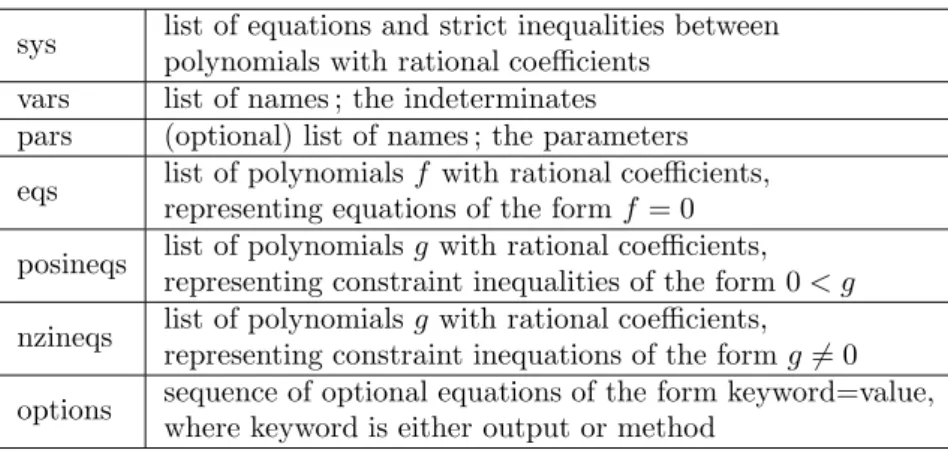
As shown in Listing 11 and Table 2, the CellDecomposition function decom-poses the parameter space of a parametric polynomial system into cells in which the original system has a constant number of solutions [29].
sys list of equations and strict inequalities between polynomials with rational coefficients
vars list of names ; the indeterminates
pars (optional) list of names ; the parameters
eqs list of polynomials f with rational coefficients,
representing equations of the form f = 0
posineqs list of polynomials g with rational coefficients,
representing constraint inequalities of the form 0 < g
nzineqs list of polynomials g with rational coefficients,
representing constraint inequations of the form g 6= 0
options sequence of optional equations of the form keyword=value,
where keyword is either output or method Table2: Description of the fields of CellDecomposition function
1 C e l l D e c o m p o s i t i o n ( s y s , v a r s , p a r s , o p t i o n s )
2 C e l l D e c o m p o s i t i o n ( eqs , p o s i n e q s , v a r s , p a r s , o p t i o n s )
3 C e l l D e c o m p o s i t i o n ( eqs , p o s i n e q s , n z i n e q s , v a r s , p a r s , o p t i o n s )
Listing 11: Architecture of Cell Decomposition
The function returns a data structure that can be used for (examples) : — Plotting the regions of the parameter space for which the system has a 340
given number of solutions.
— Extracting sample points in the parameter space for which the system has a given number of solutions.
— Extracting boxes in the parameter space in which the system has a given number of solutions.
345
The record returned captures information about the solutions of the system depending on the parameter values, including :
— a discriminant variety ;
— for each full-dimensional open cell, a sample point strictly in the interior of the cell ; if possible, the coordinates of the sample point are chosen to 350
be integers.
The input system must satisfy the following properties :
— The number of equations is equal to or greater than the number of inde-terminates ;
— At most finitely many complex solutions exist for almost all complex 355
parameter values (the system is generically zero-dimensional) ;
— For almost all complex parameter values, there are no solutions of multi-plicity greater than one (the system is generically radical) ; in particular, the input equations are square-free.
3. Manipulators Under Study 360
There are four different mechanisms for which the workspace, the joint space and the singularities are presented in this paper. Three degree of freedom parallel mechanisms consisting of three identical legs, while the different arrangements of these legs give rise to family of delta like robot. Several types of delta-like robot were studied, few of them are Orthoglide [7, 30], Hybridglide, Triaglide
[31] and UraneSX [7]. The kinematic equations of the family of delta like robot can be generalized as ||P − Bi|| = Li. These constraint equations can be in the
form of Euler angle representation or quaternions [10]. All the computations
and analysis are done for Li= L = 2 and by imposing the following constraints
on joint variables. Without joint limits, the whole family of these robots admit two assembly modes and eight working modes, i.e. ,
0 < ρ1< 2L 0 < ρ2< 2L 0 < ρ3< 2L (2)
3.1. Orthoglide Architecture and Kinematics
4 0 -4 -4 0 4 0 -4 4 A1 A2 A3 B1 B2 B3 p A1 A2 A3 B1 B2 B3 (a) (b)
Figure4: Configuration of Orthoglide : (a) simplified ; (b) real.
As shown in Fig.(4), the Orthoglide mechanism is driven by three actuated orthogonal prismatic joints. A simpler model can be defined for the Orthoglide, namely, three bar links connected by the revolute joints to the tool center point on one side and to the corresponding prismatic joint at another side. Several 365
assembly modes of these robots depends upon the solutions of direct kinematic problem (DKP). The point P represents the pose of corresponding robot. Ho-wever, more than one position for the point P shows the multiple solutions for the DKP. AiBi is equal to ρi, where ρirepresents the prismatic joint variables,
whereas P represents the position vector of the tool center point. The constraint 370
equations for the Orthoglide are :
(x − ρ1)2+ y2+ z2= L2
x2
+ (y − ρ2)2+ z2= L2
x2+ y2+ (z − ρ3)2= L2 (3)
The Maple lines used to describe this robot are as follows, shown in Listing 12
1 r o b o t:= C r e a te M a n i p u l a t o r( 2 [ ( rho1−x ) ˆ2+yˆ2+ z ˆ2− l ˆ 2 ,
3 ( rho2−y ) ˆ2+xˆ2+ zˆ2− l ˆ 2 ,
375
4 ( rho3−z ) ˆ2+xˆ2+yˆ2− l ˆ 2 ,
5 rho1 >0 , rho2 >0 , rho3 >0 ,
6 rho1 <2∗ l , rho2 <2∗ l , rho3 <2∗ l ] ,
7 [ x , y , z ] ,
8 [ rho1 , rho2 , rho3 ] ,
380
9 [ l = 1 ] ,
10 [ rho1 = −15/10..15/10 , rho2 = −15/10..15/10 ,
12 [ A1 = [ 2 ∗ l , 0 , 0 ] , A2 = [ 0 , 2∗ l , 0 ] , A3 = [ 0 , 0 , 2∗ l ] ,
13 M = [ x , y , z ] ,
385
14 B1 = [ rho1 , 0 , 0 ] , B2 = [ 0 , rho2 , 0 ] , B3 = [ 0 , 0 , rho3 ] ] ,
15 [ ] , 16 [ [ B1 , M] , [ B2 , M] , [ B3 , M] ] , 17 [ [ A1 , B1 ] , [ A2 , B2 ] , [ A3 , B3 ] ] , 18 ” O r t h o g l i d e ” ) ; 390 19 )
Listing 12: Maple lines to create the Orthoglide robot
3.2. Hybridglide Architecture and Kinematics
As shown in Fig.(5), the Hybridglide mechanism consists of three actuated prismatic joints, in which two actuators are placed parallel and third one per-pendicular to others two. Also the three bar links connected by spherical joints 395
to the tool center point on one side and to the corresponding prismatic joint at another side. Several assembly modes of these robots depends upon the solutions of the DKP. 1 -0.6 0 3 1 -1 A1 A2 A3 B1 B2 B3 A1 A2 A3 B1 B2 B3 (a) (b)
Figure5: Configuration of Hybridglide : (a) simplified ; (b) real.
The constraint equations for the Hybridglide are : (x − 1)2
+ (y − ρ1)2+ z2= L2
(x + 1)2
+ (y − ρ2)2+ z2= L2
x2+ y2+ (z − ρ3)2= L2 (4)
3.3. Triaglide Architecture and Kinematics
400 0 2 2 0 4 0 P A1 A3 B1 B2 B3 p A1 A2 A3 B1 B2 B 3 (a) (b)
As shown in Fig.(6), the Triaglide manipulator is driven by three actuated prismatic joints, in which all the three actuators all parallel to each other and placed in the same plane.
The constraint equations for the Triaglide are : (x − 1)2
+ (y − ρ1)2+ z2= L2
(x + 1)2+ (y − ρ2)2+ z2= L2
x2
+ (y − ρ3)2+ z2= L2 (5)
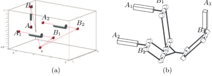
3.4. UraneSX Architecture and Kinematics
405 1 -0.6 -0.8 0.8 1 A1 A2 A3 B1 B2 p A1 A2 A3 B1 B2 B3 (a) (b)
Figure7: Configuration of UraneSX : (a) simplified ; (b) real.
As shown in Fig.(7), the UraneSX is similar to triaglide, but instead of three actuators in the same plane, they are placed in different planes. The constraint equations for the UraneSX are :
(x − 1)2+ y2 + (z − ρ1)2= L2 (x + 1/2)2 + (y −√3/2)2 + (z − ρ2)2= L2 (x + 1/2)2+ (y +√3/2)2 + (z − ρ3)2= L2 (6)
4. Singularities : Delta-Like Family Robot
Singularities of a robotic manipulator are important feature that essentially influence its motion capabilities. Mathematically, a singular configuration may be defined as rank deficiency of the Jacobian describing the differential map-ping from the joint space to the workspace and vice versa. Differentiating the constraints equations with respect to time leads to the following velocity rela-tionship :
At + B ˙q = 0 (7)
where A and B are the parallel and serial Jacobian matrices, respectively, t is 410
the velocity of P and ˙q joint velocities. The parallel singularities occur whenever det(A) = 0, while the serial singularities occur whenever det(B) = 0.
x y z x y z (a) (b) x y z x y z (c) (d)
Figure8: Projection of parallel singularity surface in the workspace for (a) Orthoglide, (b) Hybridglide, (c) Triaglide and (d) UraneSX
4.1. Parallel Singularities : Projection in workspace and joint space
Parallel singularities occur when the determinant of the direct kinematics matrix A vanishes. The corresponding singular configurations are located in-415
side the workspace. They are particularly undesirable because the manipulator can not resist any force and control is lost. Parallel singularity and its projection surfaces in workspace and joint space are calculated using the function Paral-lelSingularities(). Listing 13 shows an example for calculating the singularity surfaces and its projection in joint space.
420
1 s 2 := P a r a l l e l S i n g u l a r i t i e s ( r o b o t : : M a n i p u l a to r ) 2 s 2 c a r t := P r o j e c t i o n ( s2 , r o b o t:− P o s e V a r i a b l e s ) 3 s 2 a r t := P r o j e c t i o n ( s2 , r o b o t:− A r t i c u l a r V a r i a b l e s )
Listing 13: Projection of parallel singularity surface of delta-like robot in workspace and joint space
Parallel singularities and their projections in workspace and joint space are computed using a Gr¨obner based elimination method. This usual way for elimi-425
nating variables (see [32]) computes (the algebraic closure of) the projection of the parallel singularities in the workspace.
Eliminating variables can be done in favorable case by using cascading resultants. The main related result says that given two polynomials P, Q ∈ C[x1, . . . , xn] and their resultant R ∈ C[X1, . . . , xn−1] and α = (α1, . . . , αn−1) ∈ 430
r1 r2 r3 r1 r2 r3 (a) (b) ρ2 ρ3 ρ1 ρ2 ρ1 ρ3 (c) (d)
Figure9: Projection of parallel singularity surfaces in the joint space for (a) Orthoglide, (b) Hybridglide, (c) Triaglide and (d) UraneSX
(which means that some parts of the varieties P = 0 or Q = 0 are≪going to
in-finity≫ or ∃αn∈ C such that P (α1, . . . , αn, αn+1) = Q(α1, . . . , αn, αn+1) = 0.
Some linear change of variables allows to ignore the parts ≪ going to
infi-nity ≫ and {x ∈ Cn−1, R(x) = 0} is then the projection of V (P, Q) = {x ∈
435
Cn, P (x) = Q(x) = 0}. One can generalize this elimination step to sets of more
than two polynomials.
Taking pairs of resultants and computing their resultant with respect to xn−1
one then project again, eliminating one more variable, defining so a cascading process that will finish with univariate polynomials. This process has almost 440
the same complexity as the projection step in a CAD adapted to the input polynomials : at each step, the degree of the polynomials is doubling inducing an exponential growth (double exponential in the number of variables).
On the contrary, in favorable situations (which is our case) the discriminant variety is known to induce a lower growth of coefficients and degrees (single 445
exponential in the number of variables [33]).
Let have a look to the intersection of 3 algebraic surfaces p1(x1, x2, x3) =
p2(x1, x2, x3) = p3(x1, x2, x3) = 0 of C3 defining a finite set of points. Such a
system can also be viewed as the intersection of 3 space curves p1 = p2 = 0
, p1 = p3 = 0 and p2 = p3 = 0. By computing the resultant of each pairs
450
of polynomials wrt x3 one gets the projections of the space curves onto the
coordinates x1, x2.
A point is that the intersection of these projections might contain more points than the projection of the intersections of the space curves. It is easy to see that two space curve that do not intersect might have projections with non 455
empty intersections. The cascading process might follow with the plane curves, but (numerous) spurious points might have been introduced.
det(A)o= −ρ1ρ2ρ3+ ρ1ρ2z + ρ1ρ3y + ρ2ρ3x det(A)h= −ρ1ρ3x + ρ2ρ3x − ρ1ρ3+ ρ1z − ρ2ρ3+ ρ2z + 2ρ3y det(A)u= √ 3(3z − ρ1− ρ2− ρ3+ ρ3x + ρ2x − 2ρ1x) + 3ρ3y − 12ρ2y det(A)t= ρ1z + ρ2z − 2ρ3z (8)
In the same way, one can compute (the algebraic closure of) the projection of the parallel singularities in the joint space. Both are then defined as the zero set of some system of algebraic equations and we assume that the considered robots 460
are generic enough so that both are hypersurfaces. det(A)o, det(A)h, det(A)t
and det(A)u are the parallel singularities of Orthoglide, Hybridglide, Triaglide
and UraneSX, respectively, as shown in Eq.(8). Starting from the constraint equations and the determinant of the Jacobian matrix, we are able to eliminate the joint values. This elimination strategy is more efficient than a cascading 465
elimination by means of resultants which might introduce many more spurious solutions : singular points that are not projections of singular points.
Figure (9) shows the projections of singularity surface s2 in jointspace and s2 art is the projection surface. And s2 art is the projection curve in workspace shown in Fig.(8).
470
4.2. Serial Singularities : Projection in workspace and joint space
Serial singularities occur when the determinant of the inverse kinematics matrix B vanishes. When the manipulator is in such a singularity, there is a direction along which no Cartesian velocity can be produced. Serial singularity analysis of delta-like robot is done using the function SerialSingularities() 475
shown in Listing 14.
1 s 1 := S e r i a l S i n g u l a r i t i e s ( r o b o t : : M a n i p u l a to r ) 2 s 1 c a r t := P r o j e c t i o n ( s1 , r o b o t:− P o s e V a r i a b l e s ) 3 s 1 a r t := P r o j e c t i o n ( s1 , r o b o t:− A r t i c u l a r V a r i a b l e s )
Listing 14: Projection of serial singularities in workspace and joint space
In Eq.(9), det(B)o, det(B)h, det(B)t and det(B)u are the serial
singulari-480
ties of Orthoglide, Hybridglide, Triaglide and UraneSX, respectively. One can compute (the algebraic closure of) the projection of the serial singularities in the joint space and workspace. Both are then defined as the zero set of some system of algebraic equations and we assume that the considered robots are generic enough so that both are hypersurfaces. Also these surfaces are shown in 485
Fig.(10) and Fig.(11).
det(B)o= (ρ1− x)(ρ2− y)(ρ3− z)
det(B)h= (ρ1− y)(ρ2− y)(ρ3− z)
det(B)u= (ρ1− z)(ρ2− z)(ρ3− z)
ρ1 ρ2 ρ3 r1 r2 r3 (a) (b) ρ2 ρ3 ρ1 ρ2 ρ3 ρ1 (c) (d)
Figure10: Projection of serial singularity surfaces in the joint space for (a) Orthoglide, (b) Hybridglide, (c) Triaglide and (d) UraneSX
x y z (a) (b) x y z x y z (c) (d)
Figure11: Projection of serial singularity surfaces in the workspace for (a) Orthoglide, (b) Hybridglide, (c) Triaglide and (d) UraneSX
Figure (10) shows the projections of singularity surface s1 in joint space and s1 art is the projection surface. And s1 cart is the projection surface in works-pace and is shown in Fig.(11).
4.3. Complexity in Singularities
490
In Table 3 and 4, a comparative study of five parameters among the family of delta like robot is presented. We have tabulated the main characteristics of the polynomials (In three variables) used for the plots (Implicit surface) : their total degree, their number of terms and the maximum bitsize of their coefficients. We have also reported the time (In seconds) for plotting the implicit surface which 495
they define and the number of cells computed by the CAD, as well as the number of plotted cells where the equations admits real solutions in the plotted range.
This function is more precise than Maple’s “implicitplot3d” function because it calculates all the singular places of the surface and then triangulates it. The surface is not calculated only a discretization of the space. Several functions are 500
used which involves the discriminant variety, Gr¨obner bases and CAD compu-tations, computed in Maple 2018 with a Intel(R) Core(TM) i7-5600U CPU 2.60 GHz (16 Gb RAM). As can be seen from Table 3, there exists higher values of all the parameters for the Hybridglide, among all manipulators listed, which infers that it has more complex parallel singularities, whereas for the Triaglide all the 505
values are least which intuits the less complicated singularities. For example, the computation times for the Hybridglyde for parallel singularities is high compa-red to the one for the Othoglide, even if the surface has similar characteristics. This is due to the geometry of the surface which is more difficult to decompose in the case of the Hybridglide : the CAD is described by 636 cylindrical cells 510
in the case of Hybridglide while it is described by 300 cells for the Orthoglide because a large part of the singularity surface is a sphere.
From Table 4, it can be inferred that there exists higher values of all the pa-rameters for the UraneSX, among all manipulators listed, which infers that it has more complex serial singularities, whereas for the Triaglide all the values 515
are least which intuits the less complicated singularities. The computation times for plotting the serial singularities in joint space is higher compared to others. 5. Workspace Analysis of a Delta-like Family Robot
The workspace analysis allows to characterize of the workspace regions where the number of real solutions for the inverse kinematics is constant. A CAD 520
algorithm is used to compute the workspace of the robot in the projection space (x, y, z) with some joint constraints (shown in Eq. 2) taken in account.
The three main steps involved in the analysis are [17, 26, 34] :
— Computation of a subset of the joint space (resp. workspace) where the number of solutions changes : the Discriminant Variety .
525
— Description of the complementary of the discriminant variety in connec-ted cells : the Generic CAD.
— Connecting the cells belonging to the same connected component in the counterpart of the discriminant variety : interval comparisons.
Table 5 shows the number of cells corresponding to the number of solutions 530
Table 3: Comparison of the different parameters associated with the projection of parallel singularity surface in the workspace and joint space for the delta-like robots
PARALLEL SINGULARITIES Projection in Workspace
Manipulators Plotting Time Degrees No.of terms Binary No. of Cells
Orthoglide 07.650 18[10,10,10] 097 015 [0300,42]
Hybridglide 23.536 20[16,08,12] 119 017 [0636,80]
Triaglide 13.682 03[00,00,03] 002 002 [0150,04]
UraneSX 25.100 06[06,04,00] 015 040 [2795,66]
Projection in Joint Space
Orthoglide 00.850 06[04,04,04] 010 004 [012,01]
Hybridglide 02.917 06[04,04,04] 025 006 [111,20]
Triaglide 09.589 06[04,04,04] 041 006 [126,51]
UraneSX 02.300 06[04,04,04] 041 051 [041,09]
Table 4: Comparison of the different parameters associated with the projection of serial singularity surface in the workspace and joint space for the delta-like robots
SERIAL SINGULARITIES Projection in Workspace
Manipulators Plotting Time Degrees No.of terms Binary No. of Cells
Orthoglide 07.230 06[04,04,04] 017 006 [016,02]
Hybridglide 07.243 06[06,02,04] 015 006 [045,03]
Triaglide 05.437 06[06,06,00] 010 006 [045,03]
UraneSX 10.700 06[12,12,00] 013 036 [045,03]
Projection in Joint Space
Orthoglide 03.957 18[12,12,12] 062 012 [021,03]
Hybridglide 06.173 18[12,12,12] 281 017 [158,27]
Triaglide 06.794 06[06,06,06] 042 007 [077,17]
UraneSX 07.400 12[12,12,12] 252 151 [108,29]
Table5: Definition of the Workspace with CAD Workspace : Number of cells
Number of solutions 0 1 2 4 8 T otal
Orthoglide 28782 1196 0 0 130 30108
Hybridglide 93292 4484 7228 4196 1164 110364
Triaglide 27708 384 464 420 400 29376
UraneSX 9918 236 36 0 0 10190
shapes of workspace for the delta-like robots is shown in Fig.(12), where blue, red, yellow and green regions correspond to the one, two, four and eight number of solutions for the IKP. A comparative study is done on the workspace of the family of delta-like manipulator and the results are shown in Fig.(12). All the 535
1 IKS 2 IKS 4 IKS 8 IKS -2 2 6 -2 -2 6 x y z 2 -2 -2 -2 6 6 x y z (a) (b) -2 2 6 -2 -2 6 x y z -2 2 6 -2 -2 6 x y z (c) (d)
Figure12: Workspace plot for Orthoglide (a), Hybridglide (b), Triaglide (c) and UraneSX (d) robot
workspace are plotted in the rectangular box, where x ∈ [−2, 2], y ∈ [−2, 6] and z ∈ [−2, 6], so that the shapes of these workspace can be compared. From the Fig. 12 it can be intuited that the Triaglide will be good selection, if the task space is more in horizontal plane, whereas the Orthoglide is good for the three dimensional task space.
540
The number of cells in the workspace plays a role in motion generation when one want to know if a path is in the workspace [35]. Indeed, if we discretize the path, a Maple function named ”CellLocation” allows us to know where an pose is located from the list of cells calculated with the CAD.
6. Joint space Analysis of a Delta-like Family Robot 545
The Joint space analysis predicts the feasible and non-feasible combinations of the prismatic joint variables which are essential for the parallel robot control. The boundaries of the joint space are either the surfaces associated with the
parallel singularities or the surfaces associated with the joint limits. The Joint space analysis is done using CAD using the joint limits defined in Eq. 2. These 550
cells are plotted in Fig. (13) where red region corresponds to two solutions for the DKP. One can note that for the Orthoglide and Hybridglide robots, the shape of the joint space is regular and composed of a single connected component. For Triaglide and UraneSX robots, the joint space consists of several components either completely disconnected or connected by single lines. If we want to define 555
a robot with simple joint boundaries (defined by intervals), Orthoglide and Hybridglide robots will be the best selections.
Table 6 shows the number of cells corresponding to the number of solutions in the joint space, which is the outcome of cell decomposition. The number of cells in the joint space plays an important part while simulating robot movements 560
when control or robot geometry errors are introduced into the model. A path that can be achieved in the workspace may be too close to singular configurations after the use of the inverse geometric model including these disturbances [35]. The “CellLocation” Maple function can be used to evaluate the position of the articular trajectory. ρ1 ρ2 ρ3 ρ1 ρ2 ρ3 (a) (b) ρ1 ρ2 ρ3 ρ1 ρ2 ρ3 (c) (d)
Figure13: Joint space plot for Orthoglide (a), Hybridglide (b), Triaglide (c) and UraneSX (d) robot
Table6: Definition of the Joint space with CAD Joint space : Number of cells
Number of solutions 0 1 2 4 8 T otal
Orthoglide 10509 0 4160 0 0 14669
Hybridglide 98917 0 3041 0 0 11958
Triaglide 5375 0 426 0 0 5801
UraneSX 50598 0 4006 0 0 54604
7. Conclusions
A comparative study on the workspace of different delta-like robots gives the idea about the shape of the workspace, which further plays an important role in the selection of the manipulator for the specific task or for the trajectory plan-ning. The main characteristics associated with the singularities are tabulated in 570
Table 4 and 3 , which also gives some information about the complexity of the singularities, which is an essential factor for the singularity-free path plannings. From these data, it can be observed that the singularities associated with the Hybridglide are complicated, whereas the structure of those associated with the Triaglide is rather simple. For the Orthoglide and Hybridglide robots, the shape 575
of the joint space is regular and composed of a single connected component, whereas for Triaglide and UraneSX robots, the joint space consists of several components either completely disconnected or connected by single lines.
[1] Y. Tsai, A. Soni, An algorithm for the workspace of a general nr robot, Journal of Mechanisms, Transmissions, and Automation in Design 105 (1) 580
(1983) 52–57.
[2] J. A. Hansen, K. Gupta, S. Kazerounian, Generation and evaluation of the workspace of a manipulator, The International Journal of Robotics Research 2 (3) (1983) 22–31.
[3] C. Gosselin, Determination of the workspace of 6-dof parallel manipulators, 585
ASME Journal of Mechanical Design 112 (3) (1990) 331–336.
[4] J.-P. Merlet, Geometrical determination of the workspace of a constrained parallel manipulator, Advances in Robot Kinematics, Ferrare, Italy, Sept (1992) 7–9.
[5] G. Castelli, E. Ottaviano, M. Ceccarelli, A fairly general algorithm to eva-590
luate workspace characteristics of serial and parallel manipulators, Mecha-nics based design of structures and machines 36 (1) (2008) 14–33.
[6] I. A. Bonev, J. Ryu, A new approach to orientation workspace analysis of 6-dof parallel manipulators, Mechanism and machine theory 36 (1) (2001) 15–28.
595
[7] D. Chablat, P. Wenger, F. Majou, J.-P. Merlet, An interval analysis based study for the design and the comparison of three-degrees-of-freedom parallel kinematic machines, The International Journal of Robotics Research 23 (6) (2004) 615–624.
[8] M. Zein, P. Wenger, D. Chablat, An exhaustive study of the workspace 600
topologies of all 3r orthogonal manipulators with geometric simplifications, Mechanism and Machine Theory 41 (8) (2006) 971–986.
[9] E. Ottaviano, M. Husty, M. Ceccarelli, Identification of the workspace boundary of a general 3-r manipulator, Journal of Mechanical Design 128 (1) (2006) 236–242.
605
[10] D. Chablat, R. Jha, F. Rouillier, G. Moroz, Non-singular assembly mode changing trajectories in the workspace for the 3-rps parallel robot, in : Advances in Robot Kinematics, Springer, 2014, pp. 149–159.
[11] D. Chablat, G. Moroz, P. Wenger, Uniqueness domains and non singular as-sembly mode changing trajectories, in : Robotics and Automation (ICRA), 610
2011 IEEE International Conference on, IEEE, 2011, pp. 3946–3951. [12] R. Jha, Contributions to the performance analysis of parallel robots, Ph.D.
thesis, Ph. D. Thesis, ´Ecole Centrale de Nantes (2016).
[13] B. Siciliano, O. Khatib, Springer handbook of robotics, Springer, 2016. [14] J. Snyman, L. Du Plessis, J. Duffy, An optimization approach to the de-615
termination of the boundaries of manipulator workspaces, Journal of Me-chanical Design 122 (4) (2000) 447–456.
[15] I. A. Bonev, C. M. Gosselin, Analytical determination of the workspace of symmetrical spherical parallel mechanisms, IEEE Transactions on Robotics 22 (5) (2006) 1011–1017.
620
[16] O. Bohigas, M. Manubens, L. Ros, A complete method for workspace boun-dary determination on general structure manipulators, IEEE Transactions on Robotics 28 (5) (2012) 993–1006.
[17] D. Chablat, R. Jha, F. Rouillier, G. Moroz, Workspace and joint space analysis of the 3-rps parallel robot, in : ASME 2014 International Design 625
Engineering Technical Conferences and Computers and Information in En-gineering Conference, American Society of Mechanical Engineers, 2014, pp. V05AT08A056–V05AT08A056.
[18] R. Jha, D. Chablat, F. Rouillier, G. Moroz, Workspace and singularity ana-lysis of a delta like family robot, in : Robotics and Mechatronics, Springer, 630
2016, pp. 121–130.
[19] R. Jha, D. Chablat, L. Baron, Influence of design parameters on the singula-rities and workspace of a 3-rps parallel robot, Transactions of the Canadian Society for Mechanical Engineering 42 (1) (2018) 30–37.
[20] P. Wenger, D. Chablat, Kinetostatic analysis and solution classification of 635
a planar tensegrity mechanism, in : Computational Kinematics, Springer, 2018, pp. 422–431.
[21] G. Moroz, F. Rouiller, D. Chablat, P. Wenger, On the determination of cusp points of 3-rpr parallel manipulators, Mechanism and Machine Theory 45 (11) (2010) 1555–1567.
[22] M. Manubens, G. Moroz, D. Chablat, P. Wenger, F. Rouillier, Cusp points in the parameter space of degenerate 3-rpr planar parallel manipulators, Journal of mechanisms and robotics 4 (4) (2012) 041003.
[23] G. Moroz, D. Chablat, P. Wenger, F. Rouiller, Cusp points in the parameter space of rpr-2prr parallel manipulators, in : New Trends in Mechanism 645
Science, Springer, 2010, pp. 29–37.
[24] S. Caro, P. Wenger, D. Chablat, Non-singular assembly mode changing trajectories of a 6-dof parallel robot, in : ASME 2012 International Design Engineering Technical Conferences and Computers and Information in En-gineering Conference, American Society of Mechanical Engineers, 2012, pp. 650
1245–1254.
[25] J.-P. Merlet, Parallel robots, Vol. 128, Springer Science & Business Media, 2006.
[26] D. Lazard, F. Rouillier, Solving parametric polynomial systems, Journal of Symbolic Computation 42 (6) (2007) 636–667.
655
[27] J. Gerhard, D. Jeffrey, G. Moroz, A package for solving parametric polyno-mial systems, ACM Communications in Computer Algebra 43 (3/4) (2010) 61–72.
[28] Maple, Cylindrical Algebraic Decomposition, Vol. Maple User Manual, To-ronto : Maplesoft, a division of Waterloo Maple Inc., 2005-2015.
660
[29] Maple, Cell Decomposition, Vol. Maple User Manual, Toronto : Maplesoft, a division of Waterloo Maple Inc., 2005-2015.
[30] A. Pashkevich, D. Chablat, P. Wenger, Kinematics and workspace analysis of a three-axis parallel manipulator : the orthoglide, Robotica 24 (1) (2006) 39–49.
665
[31] M. Hebsacker, T. Treib, O. Zirn, M. Honegger, Hexaglide 6 dof and triaglide 3 dof parallel manipulators, in : Parallel kinematic machines, Springer, 1999, pp. 345–355.
[32] D. A. Cox, J. Little, D. O’shea, Using algebraic geometry, Vol. 185, Springer Science & Business Media, 2006.
670
[33] G. Moroz, Properness defects of projection and minimal discriminant va-riety, Journal of Symbolic Computation 46 (10) (2011) 1139–1157. [34] G. Moroz, Sur la d´ecomposition r´eelle et alg´ebrique des systemes d´ependant
de parametres, Ph.D. thesis, Universit´e Pierre et Marie Curie-Paris VI (2008).
675
[35] R. Jha, D. Chablat, F. Rouillier, G. Moroz, An algebraic method to check the singularity-free paths for parallel robots, in : ASME 2015 International Design Engineering Technical Conferences and Computers and Informa-tion in Engineering Conference, American Society of Mechanical Engineers, 2015, pp. V05CT08A002–V05CT08A002.