1
REGIONAL FREQUENCY ANALYSIS AT UNGAUGED SITES
1
WITH THE GENERALIZED ADDITIVE MODEL
2
F. Chebana*1, C. Charron2, T.B.M.J. Ouarda2,1 and B. Martel1 3
4 5
1
INRS-ETE, University of Quebec, 490 de la Couronne, Québec (Qc), Canada, G1K 9A9 6
2
Institute Center for Water and Environment (iWATER), 7
Masdar Institute of Science and Technology, 8
P.O.Box 54224, Abu Dhabi, UAE 9 10 11 *Corresponding author 12 Email: [email protected] 13 Tel: +1 418 654 2542 14 15 16 17 Revised version 18 19 July 2014 20
2
Abstract
21
The log-linear regression model is one of the most commonly used models to estimate flood 22
quantiles at ungauged sites within the regional frequency analysis (RFA) framework. However, 23
hydrological processes are naturally complex in several aspects including nonlinearity. The aim 24
of the present paper is to take into account this nonlinearity by introducing the generalized 25
additive model (GAM) in the estimation step of RFA. A neighbourhood approach using 26
canonical correlation analysis (CCA) is used to delineate homogenous regions. GAMs possess a 27
number of advantages such as flexibility in shapes of the relationships as well as the distribution 28
of the output variable. The regional model is applied on a dataset of 151 hydrometrical stations 29
located in the province of Québec, Canada. A stepwise procedure is employed to select the 30
appropriate physio-meteorological variables. A comparison is performed based on different 31
elements (regional model, variable selection and delineation). Results indicate that models using 32
GAM outperform models using the log-linear regression as well as other methods applied to this 33
dataset. In addition, GAM is flexible and allows including and showing non linear effects of 34
explanatory variables, in particular basin area effect (scale). Another finding is the reduced effect 35
of CCA delineation when combined with GAM. 36
37
Keywords
38
Regional frequency analysis; ungauged basin; Flood; Generalized additive model; GAM; Non-39
linear model, Canonical correlation analysis. 40
3
1. Introduction
42
Knowledge of flood characteristics is very important for resource management and design of 43
hydraulic structures. Estimation of design flows is often needed at locations where little or no 44
information is available. In this case, regional frequency analysis (RFA) is often used for the 45
estimation of flow characteristics. Ouarda et al. (2008) presented a detailed review of the various 46
available RFA methods (Blöschl et al. 2013). Generally, RFA is composed of two main steps: the 47
identification of groups of hydrologically homogeneous basins and the application of a regional 48
estimation method within each delineated region (GREHYS 1996a; Ouarda 2013). Since flow 49
characteristics are highly dependent upon physiographical and meteorological basin 50
characteristics, these can be used to estimate flood quantiles at un-gauged sites. The hydrological 51
literature abounds with studies dealing with the development and evaluation of methods for the 52
delineation of hydrological regions and for the study of their homogeneity. However, much less 53
attention has been dedicated to the development of new regional estimation methods. 54
In the present study, canonical correlation analysis (CCA) is used to delineate homogenous 55
regions. In GREHYS (1996b), it was shown that this method produced the best performances in 56
comparison to other ones. Among RFA estimation methods, regression models and index-flood 57
models are commonly used. GREHYS (1996b) showed that their performances are equivalent 58
and are superior to other models. Generally, regression models such as linear regression models 59
(LRM) or log-linear regression models (LLRM) are preferred for their simplicity and rapidity, as 60
well as their performances. LLRM has been used in conjunction with CCA in many studies 61
(Chokmani and Ouarda 2004; Ouarda et al. 2001). Linear models imply that the relations 62
between the dependent variable (hydrologic) and the predictors (physio-meteorological) are 63
linear. This is generally not realistic and can be problematic in some situations such as the effect 64
4
of the basin size on flood quantiles, where it is documented that small basins behave differently 65
than large ones. The basin hydrologic response is also not linearly related to the slope of the 66
basin, as larger basin slopes (which are often associated to smaller size basins) lead to much more 67
intense flood responses and very extreme specific peak values. 68
The generalized additive models, GAMs (Hastie and Tibshirani 1986) allow to take into account 69
possible nonlinearities which is not possible through linear models or by using simple variable 70
transformations such as log, power or square root. The use of a nonlinear model is justified by the 71
fact that hydrological processes are naturally nonlinear (Kundzewicz and Napiórkowski 1986; 72
Wittenberg 1999). Pandey and Nguyen (1999) compared a number of regional flood quantile 73
estimation methods for the power regression model (equivalently log-linear) and found that 74
nonlinear estimation methods (within the same power model) outperformed the log-linear one. 75
Shu and Ouarda (2007) used an artificial neural network approach, which represents a nonlinear 76
model, and obtained better results than with linear regression methods. 77
GAMs are an extension of the generalized linear models, GLMs (Nelder and Wedderburn 1972). 78
The latter brought flexibility to regression methods by allowing non-normal residuals as well as a 79
general link between predictors and the response variable. In addition, GAMs use non-parametric 80
smooth functions to link the dependant variable to the predictors. Therefore, they are more 81
flexible and can capture more realistically the relation between variables. GAMs have been 82
attracting high attention in statistical developments as well as in practical applications (Hastie and 83
Tibshirani 1986; Kauermann and Opsomer 2003; Marx and Eilers 1998; Morlini 2006; 84
Schindeler et al. 2009; Wood 2003). Recently, additional methodological developments and the 85
availability of implemented computer programs made GAMs increasingly popular in practical 86
research, mainly in the public health and epidemiology fields (Bayentin et al. 2010; Cans and 87
5
Lavergne 1995; Leitte et al. 2009; Rocklöv and Forsberg 2008; Vieira et al. 2009) and in 88
environmental studies (Borchers et al. 1997; Wen et al. 2011; Wood and Augustin 2002). In the 89
field of meteorology, GAMs were used to model the effect of traffic and meteorology on air 90
quality (Bertaccini et al. 2012), to predict air temperature from satellite surface temperature 91
(Kloog et al. 2012), as well as to model mean temperature in mountainous regions (Guan et al. 92
2009). In hydrological modeling, very few studies employed GAMs. For instance, Tisseuil et al. 93
(2010) used GLM and GAM for the statistical downscaling of general circulation model outputs 94
to local-scale river flows. GAMs were used to estimate nonlinear trends in water quality by 95
Morton and Henderson (2008) and in hydrological extreme series modeling by Ramesh and 96
Davison (2002). Recently, Asquith et al. (2013) employed GAMs to develop readily 97
implemented procedures for the estimation of discharge and velocity from selected predictors at 98
ungauged stream locations. However, to the author’s best knowledge, GAMs have never been 99
used in the context of RFA of hydrological variables. 100
The objective of the present study is to introduce GAMs in a complete regional model to estimate 101
flood quantiles. A set of 151 basins in the province of Québec, Canada, is considered as case 102
study. It is used in combination with the neighborhood approach using CCA. A cross validation 103
is used to evaluate performances. In previous studies dealing with the estimation of flood 104
quantiles with the same dataset (Chokmani and Ouarda 2004; Kamali Nezhad et al. 2010; Shu 105
and Ouarda 2007), explanatory variables have been selected based on correlation with specific 106
quantiles. In the present study an attempt is made to select optimal variables with a stepwise 107
method. The regional model adopting GAM is compared with a model using LLRM, which is 108
commonly used in RFA. Comparisons are also carried out for models with and without the 109
delineation of homogenous regions with CCA, and also with and without the use of the stepwise 110
6
method for the selection of variables. The latter is important to separate the impacts of using the 111
GAM model and the stepwise variable selection procedure. 112
This paper is organized as follows. Section 2 presents the theoretical background on linear 113
regression models, GAMs and the CCA approach for the delineation of neighborhoods in RFA. 114
The considered dataset as well as the study design are presented in section 3. Section 4 includes 115
the obtained results, while the last section contains the conclusions of the study. 116
2. Theoretical Background
117
In this section, the required statistical tools are briefly presented and their use in RFA is 118
discussed. 119
2.1. Linear regression models
120Regression analysis is used to find a relationship between a random variable Y, called the 121
response variable or dependant variable, and one or several random variables X, called the 122
explanatory or predictor variables (or independent variables). Let us define X, a matrix whose 123
columns are X1, X2,…, Xm,, a set of m explanatory variables. The linear regression model is
124 defined by: 125 0 1 m j j j Y β β X ε = = +
∑
+ (1) 126where
β
0 andβ
j are unknown parameters andε
is the error term which is assumed to be 127normally distributed
(
2)
0,N σ . The model parameters are often estimated by the least squares
128 estimator ˆ
(
)
1 Y β ′ − ′ = X X X . 1297
A power product model is generally used to express the relationship between flood quantiles and 130
explanatory variables (Ouarda et al. 2008; Pandey and Nguyen 1999). A log transformation 131
allows expressing this model as follows (log-linear model): 132
( )
0 1 log( ) log m j j j Y β β X ε = = +∑
+ (2) 133Note that the log transformation introduces a bias in the prediction since the aim is the estimation 134
of the variable expectation rather than its logarithm (Girard et al. 2004). 135
2.2. Generalized additive models
136The generalized linear models (GLMs) are a generalization of the well-known ordinary linear 137
model presented previously. They allows for a response distribution other than normal and for a 138
degree of nonlinearity in the model structure (Wood 2006). The GLM can be expressed as 139 follows: 140 0 1 ( ) m j j j g Y β β X ε = = +
∑
+ (3) 141where g is a monotonic link function, and Y could have whatever distribution from the 142
exponential family which includes, for instance, Poisson, Binomial and Normal distributions. 143
For more flexibility, GLMs are themselves extended to GAMs by allowing non-parametric fits of 144
the Xj where the linear forms are replaced by smooth functions fj (Hastie and Tibshirani 1986;
145 Wood 2006): 146 1 g( ) ( ) m j j j Y α f X ε = = +
∑
+ (4) 1478
GAM has several advantages over linear models. It is more flexible due to the smooth functions fj
148
where there is no need for a transformation to achieve linearity. Hence, it is possible to identify 149
more realistically the effect of each explanatory variable Xj on Y.
150
In order to estimate the smooth function fj, a spline is used. A spline is a curve composed of
151
piecewise polynomial functions, joined together at points called knots. A number of spline types 152
have been proposed in the literature, such as cubic splines, P-splines and B-splines. The thin plate 153
regression splines have some advantages such as fast computation, lack of requirement for a 154
choice of knot locations, and optimality in approximation of the smoothing, for more details see 155
(Wood 2003, 2006). In the present study, the latter splines are considered. 156
In general, a smooth function fj can be defined by a set of q spline basis functions b xji( ) such 157 that: 158 1 ( ) ( ) q j ji ji i f x
β
b x = =∑
(5) 159where
β
ji represents the smoothing coefficients related to the jth function. To avoid overfitting, 160the estimator
β
ˆ ofβ
is obtained by maximizing the penalized log-likelihood: 161 11
( )
( )
2
m T p j j jl
β
l
β
λ β
β
==
−
∑
S
(6) 162where lp(.) is the log-likelihood function,
λ
j is the smoothing parameter of the jth
smooth 163
function fj and Sj is a matrix with known coefficients (Wood 2008). The parameter
λ
jcontrols164
the smoothness degree of the curve fj. Its value ranges from 0 to 1, with 0 corresponding to the
165
un-penalised case and 1 to the completely smoothed curve. The optimum value of
λ
j is a right 1669
balance between best fitting and smoothing. The function lp(.) is maximized by the penalized
167
iteratively reweighted least squares, P-IRLS (Wood 2004). The smoothing parameter
λ
can be 168selected according to a criterion such as the generalized cross validation, GCV (Wahba 1985), 169
unbiased risk estimator, UBRE (Craven and Wahba 1978) or maximum likelihood (ML). 170
2.4. CCA Approach in RFA
171This section briefly presents the CCA approach and its connection to the delineation step of RFA. 172
This method is explained in more details in Ouarda et al. (2001) in the RFA context. Let us 173
define two sets of random variables X={X X1, 2,...,Xr} and Y={ ,Y Y1 2,..., },Ys s≥r. In the 174
present study, the set X contains basin physiographical and meteorological variables, e.g. 175
drainage area and mean annual precipitation, and Y contains basin hydrological variables such as 176
flood quantiles. In general, all variables should be standardized and transformed for normality. 177
Mainly, CCA aims to identify the dominant linear modes of covariability between the vectors X 178
and Y, and then make inference about Y given the vector X. 179
Consider the linear combinations V and W of the variables of X and Y: 180 1 1 2 2 r r a X a X a X ′ = + + + = V ⋯ a X and 1 1 2 2 s s bY b Y b Y ′ = + + + = W ⋯ b Y (7) 181
CCA allows to identify vectors a and b for which
δ
i CCA, =corr V W( ,i i) i=1,...,p are maximized 182as well as corr W V( i, j)=0, i≠ with unit variance. j 183
For each basin Bk, k =1,…,K within a given set of basins B, the corresponding values for i
V
184
and Wi are denoted as vi k, and wi k, . Let v0 denote the physio-meteorological canonical score 185
for a target site, associated to the obtained canonical variables. The vector v0 is known whereas 186
the interest is the estimation of the unknown hydrological canonical score w0. The 187
10
approximation can be obtained through Λv0such that Λ =diag(
δ
1,CCA,...,δ
p CCA, ). This leads to the 188definition of the 100(1-α)% confidence level neighbourhood for Λv0 containing sites with 189
realizations w of W such that: 190
2 1 2
0 0 ,
(w−−−−Λv ) (T Ip−−−−Λ ) (−−−− w−−−−Λv )≤≤≤≤χα p (8) 191
where Ip is the p p× identity matrix and χα2, p is such that
2 2 ,
( p) 1
P χ ≤χα = − . All the aspects α
192
related to the CCA in the RFA context are developed in Ouarda et al. (2001). 193
3. Dataset and study design
194
The considered dataset has already been studied in the context of RFA in a number of previous 195
studies (Chebana and Ouarda 2008; Chokmani and Ouarda 2004; Kamali Nezhad et al. 2010; Shu 196
and Ouarda 2007), which provides an opportunity for comparative evaluation of the results. The 197
dataset consists of 151 hydrometric stations located in the southern half of the province of 198
Québec (between 45°N and 55°N), Canada. The hydrological variables are represented by 199
specific flood quantiles (quantiles divided by the basin area), denoted by QS10, QS50 and QS100.
200
The physiographical and meteorological variables, available for each basin, are summarized in 201
Table 1. To avoid redundancy with the previously mentioned studies, details concerning the 202
dataset are not reported here. The reader is referred to the references listed above for information 203
concerning the geographic location of the stations and the scatter plots of the basins in the 204
canonical spaces. 205
The CCA in conjunction with LLRM has been proven to perform well (GREHYS 1996b). 206
However, it is suspected that the more general GAM approach can improve the estimations. In 207
this study, LLRM and GAM are compared as regional estimation models. The fitting of data for 208
11
GAM is performed with the R package mgcv (Wood 2004). Smooth parameters,
λ
jin (6), are 209estimated with the P-IRLS procedure where the ML score is employed as criterion 210
Homogenous regions are delineated with the CCA method on the basis of the variables BV, 211
PMBV, PLAC, PTMA and DJBZ. These variables are selected on the basis of maximizing
212
correlations with the hydrological variables. Since CCA requires normality, these variables are 213
transformed for the regional analysis as in the previous studies for this region, i.e. a logarithmic 214
transformation for the hydrological variables, PMBV, PTMA and DJBZ, and a square root 215
transformation for PLAC. Figure 3 (not reported here to avoid repetition) in Shu and Ouarda 216
(2007) shows clear nonlinearities in different levels for some variables. This represents a 217
motivation for the use of the GAM model with the present dataset. 218
The design of the present study aims to check the performance of three elements: i) adoption of 219
the CCA delineation step or considering all stations, ii) consideration of the nonlinearity in the 220
regression model through either LLRM or GAM during the regional estimation step and iii) the 221
variable selection method (stepwise or correlation). This leads to 8 combinations denoted as 222
follows: 223
- LLRM|ALL|CORR: LLRM with all stations (no delineation) and with the 5 selected variables 224
(from correlation); 225
- LLRM|ALL|STPW: LLRM with all stations (no delineation) and variables selected using the 226
stepwise method; 227
- LLRM|CCA|CORR: LLRM with homogeneous regions defined by CCA and with the 5 228
selected variables (from correlation); 229
- LLRM|CCA|STPW: LLRM with homogeneous regions defined by CCA and variables 230
selected using the stepwise method; 231
12
- GAM|ALL|CORR: GAM with all stations (no delineation) and with the 5 selected variables 232
(from correlation); 233
- GAM|ALL|STPW: GAM with all stations (no delineation) and variables selected using the 234
stepwise method; 235
- GAM|CCA|CORR: GAM with homogeneous regions defined by CCA and with the 5 selected 236
variables (from correlation); 237
- GAM|CCA|STPW: GAM with homogeneous regions defined by CCA and variables selected 238
using the stepwise method. 239
The selection method used in this study is the backward stepwise selection method. It starts with 240
an initial model including all available variables. The regression method is then applied with the 241
current model and the variable with the highest p-value is excluded, corresponding to the 242
hypothesis that
β
j =0 in (5) where j is the jth variable. At each step, one variable is excluded. 243The procedure ends when the p-values of all the remaining and significant variables are under a 244
given threshold (5%). 245
Once a model is established, its performance can be evaluated. A jackknife procedure is applied 246
to assess the performance of the models. In this procedure, gauged sites are in turn considered 247
ungauged in order to carry out regional estimation. This procedure allows assessing the following 248
performance criteria: 249
the coefficient of determination
2 2 1 2 1 ˆ ( ) R 1 ( ) n i i i n i i z z z z = = − = − −
∑
∑
(9) 250the root mean square error 2
1 1 ˆ RMSE ( ) n i i i z z n = =
∑
− (10) 25113
the relative root mean square error 2
1 1 ˆ rRMSE 100 ( ) / n i i i i z z z n = =
∑
− (11) 252the mean bias
1 1 ˆ BIAS ( ) n i i i z z n = =
∑
− (12) 253the relative mean bias
1 1 ˆ rBIAS 100 ( ) n i i i i z z z n = =
∑
− (13) 254 255where zi and zˆi are respectively the local (at site) and regional quantile estimates at station i, z 256
is the local mean of the hydrological variable and n is the number of stations. 257
4. Results and discussion
258
The CCA is applied on the dataset with the normalized variables BV, PMBV, PLAC, PTMA and 259
DJBZ. An optimal value of
α
=
0.05
is obtained with the optimisation procedure of Ouarda et al. 260(2001). This optimal value is used to delineate the neighborhood at each station. Each regional 261
model, when considering CCA delineation, uses the same neighbourhood for a given station. 262
When CCA is applied to the whole dataset, the two physiographical-meteorological canonical 263
variables are defined as: 264
(
)
(
)
(
)
(
)
1 0.24 log 0.07 log 0.58 0.33log 0.03log
V = BV − PMBV + PLAC− PTMA − DJBZ (14)
265
(
)
(
)
(
)
(
)
2 0.48 log 0.25log 0.45 1.05 log 1.10 log
V = BV − PMBV − PLAC + PTMA + DJBZ (15)
266
and the two hydrological canonical variables are defined as: 267
(
)
(
)
(
)
1=2.14 log 10 −13.14 log 50 +10.03 log 100
W QS QS QS (16)
268
(
)
(
)
(
)
2 =6.27 log 10 +2.45 log 50 −8.84 log 100
W QS QS QS (17)
269
The non-negligible values of the BV coefficient in V1 and V2 confirm the need to include BV in 270
the CCA despite the fact that specific hydrological quantiles are used. 271
14
The stepwise selection of variables is applied for each specific quantile separately and for each 272
regression model LLRM and GAM. Table 2 indicates that the selected variables are the same for 273
a given model and a given selection method, independently of whether CCA is used for 274
homogeneous region delineation. Therefore, the delineation step seems not to have an effect on 275
the selected variables. 276
The results of the application of the jackknife procedure for the performance evaluation of each 277
regional model are presented in Table 3. The best overall performances are obtained with 278
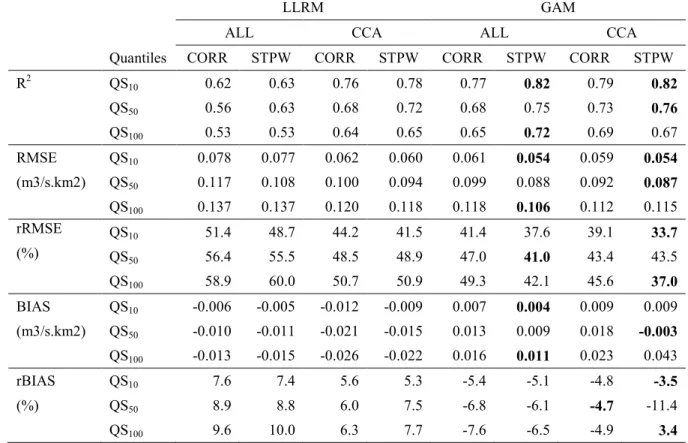
GAM|ALL|STPW and GAM|CCA|STPW with CCA leading to slightly better performances. 279
More precisely and in particular based on the rRMSE, GAM always performs better than LLRM 280
for combinations using the same variable selection approach and the same delineation approach 281
(CCA or ALL). 282
The use of CCA to delineate hydrologically homogeneous regions generally leads to 283
improvements in regional estimation in comparison to the ALL approach for the same selection 284
of variables and the same regression model (GAM or LLRM). However, when GAM is used, the 285
difference between CCA and ALL is not significant especially when using the stepwise 286
procedure for the selection of variables. These results show that the use of GAM makes the 287
procedure more robust and compensates for the advantages of using CCA. This is not the case for 288
LLRM where the use of CCA was shown to lead to significant improvements, see e.g. Chokmani 289
and Ouarda (2004). In other words, this indicates that the use of GAM reduces the importance of 290
delineating the appropriate hydrological neighborhood. A possible interpretation for this result is 291
that the consideration of non-linear formulations in the relation between the explanatory 292
physiographical and meteorological variables on one side and the hydrological variables on the 293
15
other side leads to a reduction of the weight of basins that are not hydrologically similar to the 294
target site. 295
The stepwise method for variable selection improves quantile estimations in comparison to those 296
obtained with the fixed 5 variables. This can be explained by the fact that the correlation-based 297
selection of physiographical and meteorological variables to be used in the model is mainly based 298
on a linear relationship between variables. It must also be noted that the variables are originally 299
selected for CCA purposes (delineation) rather than for regression modeling (estimation). 300
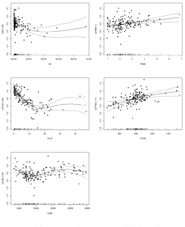
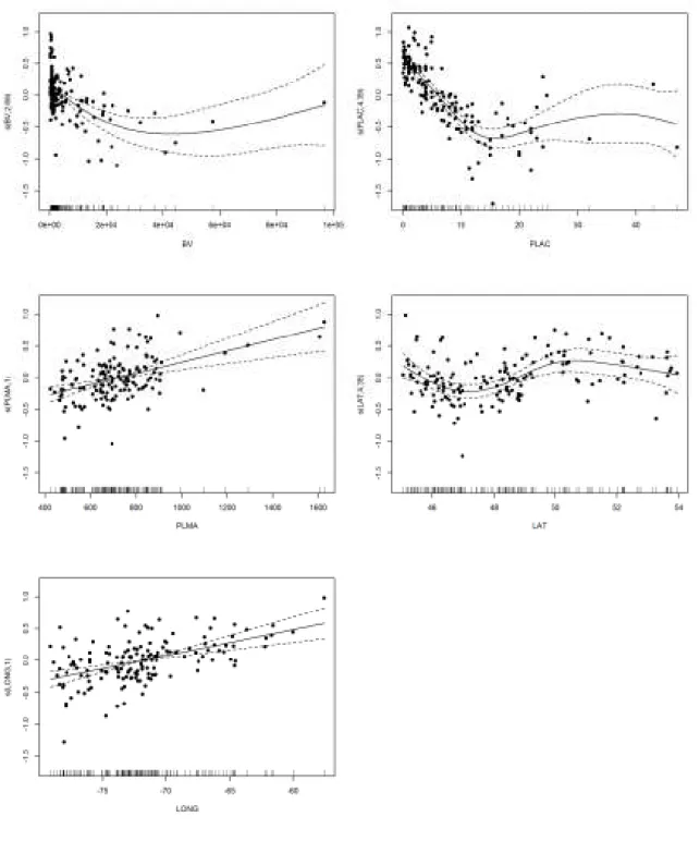
Figures 1 and 2 present the smooth functions fj of the response variable log(QS100) with the
301
explanatory variables of the fitted models GAM|ALL|CORR and GAM|ALL|STPW respectively. 302
It can be seen that the variables BV, PLAC, LAT and DJBZ show nonlinear relations. 303
Furthermore, the nonlinear relation is more complex for some variables. For instance, the 304
relationship between log(QS100) and DJBZ decreases for small values of DJBZ, increases for 305
midrange values and decreases again for high values of DJBZ. This result reflects the seasonality 306
effect of temperature, through DJBZ, on the flood regime. Another particular example of interest 307
concerns the BV variable. Indeed, it can be seen that small basins have a different effect than 308
moderate basins. This result is important since nonlinearity allows appropriately including the 309
variable BV in the model which eliminates the need to develop specific models for small, 310
moderate or large basins. Variables PMBV, LONG, PLMA and PTMA have approximately 311
linear relations. 312
In the present study, the proposed approach based on GAM is mainly compared with the basic 313
formulation of one of the most popular RFA approaches, which is the log-linear estimation model 314
combined with the CCA delineation approach. The comparison can be extended to other regional 315
flood frequency models, such as the ensemble artificial neural networks-CCA approach (EANN-316
16
CCA) (Shu and Ouarda 2007; Shu and Ouarda 2008), the kriging-CCA approach (Chokmani and 317
Ouarda 2004), and the depth-based approach (Chebana and Ouarda 2008; Wazneh et al. 2013a, 318
2013b). In order to widen the comparison, results corresponding to the above approaches are 319
considered since they are already available for the data set considered in the present study. Table 320
4 summarizes the obtained results for all these methods. The results indicate that the GAM-based 321
approach outperforms significantly all the above listed approaches in terms of rRMSE. In terms 322
of rBIAS, the optimal depth-based approach seems to lead to slightly better results, although the 323
difference is not significant. 324
5. Conclusions
325
GAM is commonly used in health, epidemiological and environmental studies. However, it 326
remains unutilized in the field of hydrology, especially in RFA. The multiple linear regression 327
model is the most employed estimation model in RFA mainly because of its simplicity. However, 328
it assumes a log linear relationship between the response variable and the explanatory variables. 329
This assumption is not always true and does not reflect the complexity of the hydrological 330
processes involved. The purpose of the present study is first to introduce GAM in RFA and then 331
to compare its results with those obtained by LLRM. GAM is a flexible model that relaxes the 332
assumptions of the LLRM model (normality and linearity). 333
Results of this study indicate that significantly better estimations are obtained from regional 334
models with GAM. For some explanatory variables, the logarithmic relationship of the response 335
variable with the explanatory variables is not linear. Smooth curves allow for a more realistic 336
understanding of the true relationship between response and explanatory variables. The 337
performance gain is not significant using CCA in conjunction with GAM compared to LLMR. 338
This indicates that GAM is robust and is efficient in RFA even without use of a neighborhood 339
17
approach. Further efforts are required to generalize this conclusion and to test the benefits of 340
GAM modeling in other hydrological applications. 341
In summary, the use of GAM in RFA is valuable not only in terms of performance but also in 342
terms of other practical aspects (e.g. explicit formulation of the smooth functions, flexibility, 343
reduced number of assumptions, and less subjective choices). 344
Acknowledgments
345Financial support for this study was graciously provided by the Natural Sciences and Engineering 346
Research Council (NSERC) of Canada, under funding to the Canada Research Chair on the 347
Estimation of Hydro-Meteorological variables. The authors thank the ministry of the environment 348
of Quebec (MENVIQ) services for the employed data sets. For confidentiality reasons, the data 349
cannot be released. The authors are grateful to the Editor and the anonymous reviewers for their 350
valuable comments and suggestions. 351
18
References
352
Asquith, W. H., G. R. Herrmann, and T. G. Cleveland, 2013: Generalized Additive Regression 353
Models of Discharge and Mean Velocity Associated with Direct-Runoff Conditions in Texas: 354
Utility of the U.S. Geological Survey Discharge Measurement Database. Journal of Hydrologic 355
Engineering, 18, 1331-1348.
356
Bayentin, L., S. El Adlouni, T. B. M. J. Ouarda, P. Gosselin, B. Doyon, and F. Chebana, 2010: 357
Spatial variability of climate effects on ischemic heart disease hospitalization rates for the period 358
1989-2006 in Quebec, Canada. International Journal of Health Geographics, 9. 359
Bertaccini, P., V. Dukic, and R. Ignaccolo, 2012: Modeling the short-term effect of traffic and 360
meteorology on air pollution in turin with generalized additive models. Advances in Meteorology, 361
2012.
362
Blöschl, G., M. Sivapalan, T. Wagener, A. Viglione, and H. Savenije, 2013: Runoff prediction in 363
ungauged basins. Synthesis across processes, places and scales. Cambridge University Press.
364
Borchers, D. L., S. T. Buckland, I. G. Priede, and S. Ahmadi, 1997: Improving the precision of 365
the daily egg production method using generalized additive models. Canadian Journal of 366
Fisheries and Aquatic Sciences, 54, 2727-2742.
367
Cans, C., and C. Lavergne, 1995: De la régression logistique vers un modèle additif généralisé : 368
un exemple d'application. Revue de Statistique Appliquée, 43, 77-90. . 369
Chebana, F., and T. B. M. J. Ouarda, 2008: Depth and homogeneity in regional flood frequency 370
analysis. Water Resour. Res., 44, W11422. 371
Chokmani, K., and T. B. J. M. Ouarda, 2004: Physiographical space-based kriging for regional 372
flood frequency estimation at ungauged sites. Water Resour. Res., 40, W12514. 373
Craven, P., and G. Wahba, 1978: Smoothing noisy data with spline functions. Numer. Math., 31, 374
377-403. 375
Girard, C., T. B. M. J. Ouarda, and B. Bobée, 2004: Study of the bais in the log-linear regional 376
estimation model. Can. J. Civ. Eng., 31, 361-368. 377
GREHYS, 1996a: Presentation and review of some methods for regional flood frequency 378
analysis. Journal of Hydrology, 186, 63-84. 379
——, 1996b: Inter-comparison of regional flood frequency procedures for Canadian rivers. 380
Journal of Hydrology, 186, 85-103.
381
Guan, B. T., H. W. Hsu, T. H. Wey, and L. S. Tsao, 2009: Modeling monthly mean temperatures 382
for the mountain regions of Taiwan by generalized additive models. Agricultural and Forest 383
Meteorology, 149, 281-290.
384
Hastie, T., and R. Tibshirani, 1986: Generalized Additive Models. Statistical Science, 1, 297-310. 385
Kamali Nezhad, M., K. Chokmani, T. Ouarda, M. Barbet, and P. Bruneau, 2010: Regional flood 386
frequency analysis using residual kriging in physiographical space. Hydrological Processes, 24, 387
2045-2055. 388
Kauermann, G., and J. D. Opsomer, 2003: Local Likelihood Estimation in Generalized Additive 389
Models, 30, 317-337. 390
Kloog, I., A. Chudnovsky, P. Koutrakis, and J. Schwartz, 2012: Temporal and spatial 391
assessments of minimum air temperature using satellite surface temperature measurements in 392
Massachusetts, USA. Science of the Total Environment, 432, 85-92. 393
Kundzewicz, Z. W., and J. J. Napiórkowski, 1986: Non linear models of dynamic hydrology. 394
Hydrological Sciences Journal-Journal Des Sciences Hydrologiques, 31, 163-185.
19
Leitte, A. M., and Coauthors, 2009: Respiratory health, effects of ambient air pollution and its 396
modification by air humidity in Drobeta-Turnu Severin, Romania. Science of The Total 397
Environment, 407, 4004-4011.
398
Marx, B. D., and P. H. C. Eilers, 1998: Direct generalized additive modeling with penalized 399
likelihood. Computational Statistics & Data Analysis, 28, 193-209. 400
Morlini, I., 2006: On Multicollinearity and Concurvity in Some Nonlinear Multivariate Models. 401
Statistical Methods & Applications, 15, 3-26.
402
Morton, R., and B. L. Henderson, 2008: Estimation of nonlinear trends in water quality: An 403
improved approach using generalized additive models. Water Resour. Res., 44. 404
Nelder, J. A., and R. W. M. Wedderburn, 1972: Generalized Linear Models. Journal of the Royal 405
Statistical Society. Series A (General), 135, 370-384.
406
Ouarda, T. B. M. J., 2013: Regional Hydrological Frequency Analysis. Encyclopedia of 407
Environmetrics, John Wiley & Sons, Ltd.
408
Ouarda, T. B. M. J., A. St-Hilaire, and B. Bobée, 2008: Synthèse des développements récents en 409
analyse régionale des extrêmes hydrologiques / A review of recent developments in regional 410
frequency analysis of hydrological extremes. Revue des sciences de l'eau / Journal of Water 411
science, 21, 219-232.
412
Ouarda, T. B. M. J., C. Girard, G. S. Cavadias, and B. Bobee, 2001: Regional flood frequency 413
estimation with canonical correlation analysis. Journal of Hydrology, 254, 157-173. 414
Pandey, G. R., and V. T. V. Nguyen, 1999: A comparative study of regression based methods in 415
regional flood frequency analysis. Journal of Hydrology, 225, 92-101. 416
Ramesh, N. I., and A. C. Davison, 2002: Local models for exploratory analysis of hydrological 417
extremes. Journal of Hydrology, 256, 106-119. 418
Rocklöv, J., and B. Forsberg, 2008: The effect of temperature on mortality in Stockholm 1998-419
2003: A study of lag structures and heatwave effects. Scandinavian Journal of Public Health, 36, 420
516-523. 421
Schindeler, S., D. Muscatello, M. Ferson, K. Rogers, P. Grant, and T. Churches, 2009: 422
Evaluation of alternative respiratory syndromes for specific syndromic surveillance of influenza 423
and respiratory syncytial virus: a time series analysis. BMC Infectious Diseases, 9, 190. 424
Shu, C., and T. B. J. M. Ouarda, 2007: Flood frequency analysis at ungauged sites using artificial 425
neural networks in canonical correlation analysis physiographic space. Water Resour. Res., 43, 426
W07438. 427
Shu, C., and T. B. M. J. Ouarda, 2008: Regional flood frequency analysis at ungauged sites using 428
the adaptive neuro-fuzzy inference system. Journal of Hydrology, 349, 31-43. 429
Tisseuil, C., M. Vrac, S. Lek, and A. J. Wade, 2010: Statistical downscaling of river flows. 430
Journal of Hydrology, 385, 279-291.
431
Vieira, V., T. Webster, J. Weinberg, and A. Aschengrau, 2009: Spatial analysis of bladder, 432
kidney, and pancreatic cancer on upper Cape Cod: an application of generalized additive models 433
to case-control data. Environmental Health, 8, 3. 434
Wahba, G., 1985: A comparison of GCV and GML for choosing the smoothing parameter in the 435
generalized spline smoothing problem. Ann. Stat., 13, 1378-1402. 436
Wazneh, H., F. Chebana, and T. B. M. J. Ouarda, 2013a: Optimal depth-based regional frequency 437
analysis. Hydrology and Earth System Sciences, 17, 2281-2296. 438
——, 2013b: Depth-based regional index-flood model. Water Resour. Res., In presss. 439
Wen, L., K. Rogers, N. Saintilan, and J. Ling, 2011: The influences of climate and hydrology on 440
population dynamics of waterbirds in the lower Murrumbidgee River floodplains in Southeast 441
20
Australia: Implications for environmental water management. Ecological Modelling, 222, 154-442
163. 443
Wittenberg, H., 1999: Baseflow recession and recharge as nonlinear storage processes. 444
Hydrological Processes, 13, 715-726.
445
Wood, S. N., 2003: Thin plate regression splines. J. R. Stat. Soc. Ser. B-Stat. Methodol., 65, 95-446
114. 447
——, 2004: Stable and efficient multiple smoothing parameter estimation for generalized 448
additive models. Journal of the American Statistical Association, 99, 673-686. 449
——, 2006: Generalized Additive Models: An Introduction with R. Chapman and Hall/CRC 450
Press, 392 pp. 451
——, 2008: Fast stable direct fitting and smoothness selection for generalized additive models. J. 452
R. Stat. Soc. Ser. B-Stat. Methodol., 70, 495-518.
453
Wood, S. N., and N. H. Augustin, 2002: GAMs with integrated model selection using penalized 454
regression splines and applications to environmental modelling. Ecological Modelling, 157, 157-455
177. 456
21
Table 1. Descriptive statistics of hydrological variables and physio-meteorological variables. 457
Variable Unit Notation Min Moy Max SD
Specific flood of 10 year return period m³/s.km² QS10 0.03 0.22 0.53 0.13
Specific flood of 50 year return period m³/s.km² QS50 0.03 0.28 0.77 0.18
Specific flood of 100 year return period m³/s.km² QS100 0.03 0.31 0.94 0.20
Area of Watershed km2 BV 208 6 265 96 600 11 713
Length of main channel km LCP 17 157 855 142
Slope of main channel m/km PCP 0.20 3.23 23.60 3.22
Mean slope of watershed ° PMBV 0.96 2.43 6.81 0.99
Percentage of the basin occupied by forest % PFOR 18.00 83.05 99.80 16.61 Percentage of the basin occupied by lakes % PLAC 0.03 7.72 47.00 7.99
Mean annual total precipitations mm PTMA 646 988 1 534 154
Mean annual liquid precipitations mm PLMA 423 717 1625 176
Mean annual solid precipitations cm PSMA 166 302 720 86
Mean annual liquid precipitations during summer and fall
PLME 306 455 664 72 Mean annual degree-days over 0°C dgr-day DJBZ 8 589 16 346 29 631 5 385
Latitude of the station ° LAT 45 48 54 2
Longitude of the station ° LONG 58 72 79 4
Altitude of the station m ALT 5 157 555 125
458
Table 2. Variables selected for each regional model. 459
Regional Models Quantile Selected explanatory variables
[LLRM|ALL|STPW], [LLRM|CCA| STPW] QS10 BV, PMBV, PFOR, PLAC, PLMA, DJBZ, LONG
QS50 BV, PMBV, PFOR, PLAC, PLMA, LONG
QS100 BV, PLAC, PLMA, LONG
[GAM|ALL|STPW], [GAM|CCA|STPW] QS10 BV, PFOR, PLAC, PTMA, LAT, LONG
QS50 BV, PLAC, PLMA, LAT, LONG
QS100 BV, PLAC, PLMA, LAT, LONG
[LLRM|ALL|CORR], [LLRM|CCA|CORR], [GAM|ALL|CORR], [GAM|ALL|CORR] QS10 BV, PMBV, PLAC, PTMA, DJBZ QS50 BV, PMBV, PLAC, PTMA, DJBZ QS100 BV, PMBV, PLAC, PTMA, DJBZ 460 461
22
Table 3. Performances obtained with the eight combinations (model, delineation and variable 462
selection). 463
LLRM GAM
ALL CCA ALL CCA
Quantiles CORR STPW CORR STPW CORR STPW CORR STPW
R2 QS10 0.62 0.63 0.76 0.78 0.77 0.82 0.79 0.82 QS50 0.56 0.63 0.68 0.72 0.68 0.75 0.73 0.76 QS100 0.53 0.53 0.64 0.65 0.65 0.72 0.69 0.67 RMSE QS10 0.078 0.077 0.062 0.060 0.061 0.054 0.059 0.054 (m3/s.km2) QS50 0.117 0.108 0.100 0.094 0.099 0.088 0.092 0.087 QS100 0.137 0.137 0.120 0.118 0.118 0.106 0.112 0.115 rRMSE QS10 51.4 48.7 44.2 41.5 41.4 37.6 39.1 33.7 (%) QS50 56.4 55.5 48.5 48.9 47.0 41.0 43.4 43.5 QS100 58.9 60.0 50.7 50.9 49.3 42.1 45.6 37.0 BIAS QS10 -0.006 -0.005 -0.012 -0.009 0.007 0.004 0.009 0.009 (m3/s.km2) QS50 -0.010 -0.011 -0.021 -0.015 0.013 0.009 0.018 -0.003 QS100 -0.013 -0.015 -0.026 -0.022 0.016 0.011 0.023 0.043 rBIAS QS10 7.6 7.4 5.6 5.3 -5.4 -5.1 -4.8 -3.5 (%) QS50 8.9 8.8 6.0 7.5 -6.8 -6.1 -4.7 -11.4 QS100 9.6 10.0 6.3 7.7 -7.6 -6.5 -4.9 3.4
Best performances are in bold character for each criterion and quantile
464 465
Table 4. Results of several RFA approaches applied to the same data set considered in this study 466
QS10 QS100
Method References rBIAS
(%) rRMSE (%) rBIAS (%) rRMSE (%)
Linear regression Table 3 above -9 55 -11 64
Nonlinear regression Shu and Ouarda 2008 -9 61 -12 70
Nonlinear regression with regionalization approach Shu and Ouarda 2008 -19 67 -24 79
Linear regression-CCA Table 3 above -7 44 -8 52
Kriging in the CCA Physiographical Space Chokmani and Ouarda 2004 -20 66 -27 86 Kriging in the PCA Physiographical Space Chokmani and Ouarda 2004 -16 51 -23 70
Adaptive Neuro-Fuzzy Inference Systems Shu and Ouarda 2008 -8 57 -14 64
Artificial Neural Networks Shu and Ouarda 2008 -8 53 -10 60
Single Artificial Neural Networks-CCA space Shu and Ouarda 2007 -5 38 -4 46
Ensemble Artificial Neural Networks Shu and Ouarda 2007 -7 44 -10 60
Ensemble Artificial Neural Networks -CCA space Shu and Ouarda 2007 -5 37 -6 45
Optimal depth-based approach Wazneh et al. 2013a -3 38 -2 44
GAM|CCA|STPW Table 3 above -3.5 33.7 3.4 37
23 467
Figure 1. Smooth functions of QS100 for the explanatory variables included in the regional model
468
GAM|ALL|CORR. The dotted lines represent the 95% confidence intervals. The y-axes are 469
named s(var,edf) where var is the name of the explanatory variable and edf is the estimated 470
degree of freedom of the smooth. 471
24 472
Figure 2. Smooth functions of QS100 for the explanatory variables included in the regional model
473
GAM|ALL|STPW. The dotted lines represent the 95% confidence intervals. The y-axes are 474
named s(var,edf) where var is the name of the explanatory variable and edf is the estimated 475
degree of freedom of the smooth. 476