1
Regional low-flow frequency analysis with a recession parameter from a
non-1linear reservoir model
23
Christian Charron1, * and Taha B.M.J. Ouarda1, 2 4
5 1
Institute Center for Water and Environment (iWATER), Masdar Institute of Science and 6
Technology, P.O. Box 54224, Abu Dhabi, UAE 7
2
INRS-ETE, National Institute of Scientific Research, Quebec City (QC), G1K9A9, Canada 8 9 10 11 12 13 14 15
*Corresponding author: Email: [email protected] 16 Tel: +971 2 810 9524 17 18 19 20 21 22 23
Submitted to Journal of Hydrology 24
February 2015 25
2
Abstract: Several studies have shown that improvements in the regional prediction of low-27
flow characteristics can be obtained through the inclusion of a parameter characterising 28
catchment baseflow recession. Usually, a linear reservoir model is assumed to define 29
recession characteristics used as predictors in regional models. We propose in this study to 30
adopt instead a non-linear model. Predictors derived from the linear model and the non-linear 31
model are used separately in low-flow regional models along with other predictors 32
representing physiographical and meteorological characteristics. These models are applied to 33
selected gaged catchments. Results show that better performances are obtained with the 34
parameter from the non-linear model. One drawback of using recession parameters for 35
regional estimation is that a streamflow record is required at the site of interest. However, 36
recession parameters can be estimated with short streamflow records. In this study, to 37
simulate the performances obtained at partially gaged catchments, the recession parameters 38
are estimated with very short streamflow records at target sites. Results indicate that, with a 39
streamflow record as short as one year, a model with a recession parameter from the non-40
linear model leads to better performances than a model with only physiographical and 41
meteorological characteristics. 42
43
Keywords: Regional estimation; Low-flows; Recession analysis; Canonical correlation 44
analysis; Non-linear model; Reservoir model. 45
46 47
3
1. Introduction
48
It is of major importance to engineers and water managers to properly estimate the 49
frequency of low-flow events, and their spatial and temporal evolution in the region of study 50
(Vogel and Kroll, 1992; Durrans et al., 1999; Smakhtin, 2001; Kroll et al., 2004; Khaliq et al., 51
2008, 2009; Ouarda et al., 2008b; Fiala et al., 2010). Applications where this information is 52
needed include water supply, hydropower production, dilution of pollution discharge and 53
aquatic wildlife protection. The most commonly used low-flow statistic is the quantile Qd, T 54
defined as the annual minimum average streamflow during d days with a return period of T 55
years. When a sufficient historical streamflow record is available at a given site, low-flow 56
statistics are obtained with a frequency analysis using the observed streamflow data. 57
However, when insufficient or no streamflow record is available, a regional approach needs to 58
be employed (Hamza et al., 2001; Ouarda et al., 2001; Kroll et al., 2004). 59
For the purpose of regional estimation, regression models are often used to estimate low-flow 60
quantiles with explanatory variables characterising physiographical catchment properties and 61
meteorological conditions. It has been demonstrated that explanatory variables representing 62
geological and hydrogeological characteristics have a strong influence on low-flow regimes 63
(Bingham, 1986; Tallaksen, 1989; Vogel and Kroll, 1992; Smakhtin, 2001; Kroll et al., 2004). 64
However, such variables are hard to establish and difficult to quantify (Demuth and 65
Hagemann, 1994). To address this issue, many authors have used baseflow recession 66
parameters as surrogate to these variables (Bingham, 1986; Tallaksen, 1989; Arihood and 67
Glatfelter, 1991; Vogel and Kroll, 1992, 1996; Demuth and Hagemann, 1994; Kroll et al., 68
2004; Eng and Milly, 2007). This is justified by the fact that low flows result principally of 69
groundwater discharge into the stream during dry periods. 70
4
In studies where recession parameters were used to estimate low-flow statistics, a linear 71
reservoir model is always assumed. This approximation is used for convenience, but a non-72
linear relation is more accurate in general (Brutsaert and Nieber, 1977; Whittenberg, 1994; 73
Chapman, 2003). In this study, we propose to use a recession parameter assuming the non-74
linear reservoir model in a regional model along with other physiographical and 75
meteorological characteristics for the estimation of low-flow quantiles. Performances are 76
compared with those with a regional model including instead a parameter that assumes the 77
common linear reservoir model. The regional models are applied to a group of catchments in 78
the province of Quebec (Canada). 79
A major inconvenience of using recession parameters as predictors is that hydrological data is 80
needed at the site of interest. However, they can be estimated with a short streamflow time 81
series when it is available at the site of interest. A second objective of this paper is to evaluate 82
the potential of this method at such sites (referred to as partially gaged sites). For that, a 83
partially gaged case is simulated at the target site by estimating the recession parameters with 84
only few years of streamflow record data selected randomly from the complete streamflow 85
record. 86
Regional frequency analysis involves usually two steps: the identification of groups of 87
hydrologically homogeneous catchments and the regional estimation within each individual 88
region. In this study, canonical correlation analysis (CCA) is used to delineate the 89
homogenous regions. This method has been used with success for the regionalization of flood 90
quantiles (Ouarda et al., 2001), low-flow quantiles (Tsakiris et al., 2011) and water quality 91
characteristics (Khalil et al., 2011). 92
5
2. Recession curve modeling
94
Boussinesq (1877) conceptualised the problem of outflow into a penetrating stream 95
channel from an unconfined rectangular aquifer on a horizontal impermeable layer. Brutsaert 96
and Nieber (1977) demonstrated that several solutions to the Boussinesq problem assume the 97 following relation: 98 b dQ aQ dt (1) 99
where Q is the streamflow, t is the time, and a [m3(1-b)sb-2] and b [-] are constants. 100
The linear reservoir model in which b1 is often considered. The solution of Eq. (1) for the 101
outflow is then the simple exponential equation: 102 0 at t Q Q e (2) 103
where Q is the outflow at time t and t Q the initial outflow. Eq. (2) in its exponential form is 0 104
often used to describe recession curves because of its simplicity. In that case, a characterises 105
the rate of recession. Many authors have used parameters derived from the linear model as 106
predictors in regression models. Vogel and Kroll (1992) and Kroll et al. (2004) used the 107
recession constant Kb exp(a). Eng and Milly (2007) rather used the parameter a1 to 108
which they referred as the long-term aquifer constant. 109
Although the linear reservoir model has been largely employed, the power-law model is more 110
appropriate. In several studies where non-linear equations have been fitted to recession 111
discharge data, it was found that the power-law model is more realistic (Moore, 1997; 112
Chapman, 1999, 2003; Wittenberg, 1999). Brutsaert and Nieber (1977) found that b takes 113
approximately the value of 1.5 over most of the ranges of low-flow rates. The value of the 114
6
exponent b ranged from 1.38 to 1.69 for 10 out of 11 catchments in Chapman (2003). In 115
Wittenberg (1994) a mean value of 1.6 was obtained. 116
We propose in this study to use a parameter derived from the non-linear reservoir model 117
instead of the usually used linear model. Because b is different from 1 in general, it is 118
expected that the performances will be increased by the use of this optimised parameter in 119
regional models. Wittenberg (1999) stated that a value of 1.5 is a typical value for average 120
cases and suggested to calibrate the factor a with b fixed to this value. In this study, a is 121
estimated with a fixed value of b for the whole study area estimated by the average of 122
individual catchment values. To estimate b for a given catchment, a similar approach to Vogel 123
and Kroll (1992) and Brutsaert and Lopez (1998) is used. The relation in Eq. (1) is 124 approximated by: 125 1 1 2 b t t t t Q Q Q Q a t (3) 126
where Q and t Qt1 are the streamflow measurements at successive times t apart. By taking 127
the logarithm, the following linearised equation is obtained: 128 1 1 ln( ) ln( ) ln 2 t t t t Q Q Q Q a b . (4) 129
The parameter b along with the parameter a in Eq. (4) are estimated using a least square linear 130
regression. Subsequently, given a fixed value of b, the least square estimator of a in Eq. (4) is 131 given by: 132 1 1 1 1 exp ln( ) ln 2 d t t t t t Q Q a Q Q b d
(5) 133where d is the number of pairs of consecutive streamflow values. 134
7 135
3. Study area
136
The regional proposed estimation models are applied to a network of 190 gaging 137
stations in the province of Quebec (Canada). Due to the seasonal variations specific to the 138
study area, we consider two distinct low-flow seasons corresponding to the summer and the 139
winter. In this study, we analyse the low-flow quantiles Q7, 2 and Q7, 10corresponding to return 140
periods of T = 2 and 10 years for a duration d = 7 days, and the low-flow quantile Q30, 5 141
corresponding to a return period of T = 5 years for a duration d = 30 days for the summer and 142
winter seasons separately. The hydrological, physiographical and meteorological variables 143
used in the present case study came from a low-flow frequency analysis study by Ouarda et al. 144
(2005). The same database has also been used in Ouarda and Shu (2009) for low-flow 145
frequency analysis using artificial neural networks. Only stations with at least 10 years of 146
record data and corresponding to pristine basins were selected. The selected stations passed 147
the Kendall test for stationarity, the Wald-Wolfowitz test of independence, the Wilcoxon test 148
of homogeneity for the mean and the Levene test for homogeneity of the variance. As a result, 149
127 and 133 stations were selected for the summer season and the winter season respectively. 150
The locations of the gaging stations are presented in Fig. 1. The stations cover a large area in 151
the southern part of the province of Quebec (Canada) and are located between 45°N and 152
55°N. The area of the catchments ranges from 0.7 km2 to 96,600 km2 with a median value of 153
3077 km2. The largest catchments are located in the northern part of the study region. The 154
average flow record size is 32 years of data. Winter mean temperatures for the study area 155
range from -10°C in the south to -21°C in the north and summer mean temperatures range 156
from 20°C in the south to 12°C in the north. 157
8
A set of physiographical and meteorological variables are available for each basin. These 158
variables are the basin area (AREA), the latitude of the gaging station (LAT), the mean slope 159
of the drainage area (MSLP), the percentage of the basin area occupied by lakes (PLAKE), 160
the percentage of the basin area covered by forest (PFOR), the mean annual degree days 161
below 0ºC (DDBZ), the mean annual degree days below 0ºC (DDH13), the average annual 162
precipitation (PTMA), the average summer-autumn liquid precipitation (PLMS), the average 163
number of days for which the mean temperature exceeds 27 ºC (NDH27) and the mean curve 164
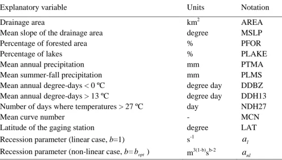
number (MCN) which is a soil characteristic. These variables are summarised in Table 1. 165
Low-flow quantiles corresponding to various return periods T and durations d were estimated. 166
Low-flow data at each station was fitted with an appropriate statistical distribution. The 167
distributions considered include the Generalized Extreme Value, Gumbel, Weibull, two-168
parameter Lognormal, three-parameter Lognormal, Gamma, Pearson type III, Log-Pearson III 169
and Generalized Pareto distributions. To select the distribution that best fits the hydrological 170
data for each station, the Bayesian information criterion was used. Fig. 2 presents an example 171
of a frequency curve with the observed data on a normal probability plot. The distribution that 172
fits best the observations, the two-parameter Lognormal (LN2), is represented along with the 173
bounds of the 95% confidence interval. 174
175
4. Study methodology
176
4.1. Recession analysis method
177
The computation of recession characteristics at gaged sites is usually done through a 178
recession analysis. This involves the delineation of baseflow recession segments from 179
hydrographs and subsequently the computation of recession characteristics. In practice, the 180
9
interpretation of hydrographs is complicated by the fact that, during a recession period, 181
recharge events can often interrupt a recession and produce many recession segments of 182
different lengths. Another interpretative complication comes from the fact that the different 183
streamflow components, that are surface flow, interflow and baseflow, are difficult to quantify 184
at a given time. Given these considerations, various researchers have developed methods to 185
delineate baseflow recession segments from hydrographs. 186
Traditionally, graphical techniques are used for recession analysis. They are however 187
subjective and applicable only for a few analyses because they are time consuming. For a 188
large database, automated methods are preferred. Several methods have been proposed in the 189
literature. They usually take only decreasing portions of hydrographs in which starting and 190
duration criteria are defined. The minimal length of individual recession segments can usually 191
vary between 4 days and 10 days (Tallaksen, 1995). A portion at the beginning of recession 192
segments can also be removed to avoid the presence of surface flow. 193
The recession analysis method applied here is based on the procedure proposed by Vogel and 194
Kroll (1992) in which segments of only decreasing 3-day moving average are selected. Only 195
segments with a minimum of 10 days are considered. Furthermore, to minimise surface runoff 196
components, 30 % of the beginning of each segment is subtracted. 197
The recession parameter a is defined for the non-linear reservoir model. It is computed at nl 198
each catchment with b fixed to bopt , the optimal value for the whole study area. bopt is
199
estimated by averaging the estimated values of b at each basin. The recession variable a for l 200
the linear reservoir model is also estimated. In that case, b is set to unity (b = 1) for the whole 201
area. 202
4.2. Delineation of homogenous regions with CCA
10
Regionalization methods usually involve two steps: defining groups of homogeneous 204
stations and applying an information transfer method over the delineated regions. As in the 205
case of flood regionalization, grouping stations provides generally better estimates because 206
stations in the same group are expected to have similar hydrological responses. Certain 207
delineation methods allow defining geographically contiguous regions. This kind of approach 208
can involve the delineation on the basis of geographic considerations or on the basis of the 209
similitude in residuals obtained by a regression model (Smakhtin, 2001). In reality, two basins 210
can be hydrologically similar without being geographically close. Other methods allow 211
defining groups of catchments that are not necessarily contiguous. Delineation is then made 212
on the basis of the physiographic and climatic characteristics of the catchments. Multivariate 213
statistical analysis methods such as cluster analysis and principal component analysis are then 214
often used (Nathan and McMahon, 1990; Smakhtin, 2001). 215
Another promising multivariate approach is canonical correlation analysis (CCA). It has been 216
applied in the field of flood regionalization by Ouarda et al. (2000, 2001) and it has been 217
proven to be applicable for low flow regionalization in Tsakiris et al. (2011). This method 218
defines for each target station, a specific set of homogenous stations (neighbourhood). This 219
has the advantage of maximising the similarity between the neighbourhood catchments and 220
the target site. The neighbourhood approach was found in Ouarda et al. (2008a) to be superior 221
to approaches delineating fixed sets of stations for regional flood frequency analysis. 222
Optimal neighbourhoods need to be delineated for models where a CCA is involved. The 223
jackknife resampling procedure presented in Ouarda et al. (2001) is used. However, when a 224
neighbourhood is defined by the optimisation parameter, it may happen that the number of 225
stations in the neighbourhood is not large enough to be able to carry out the multiple 226
regression. The jackknife resampling procedure is modified in this study to include instead the 227
11
s stations with the lowest Mahalanobis distance. This ensures that estimations are obtained at 228
all stations of the study area. 229
4.3. Regional models
230
Overall, six regional models are defined depending on which explanatory variables are 231
used and whether neighbourhoods are delineated or not. For three models (ALL , ALL_a l 232
and ALL_a ), the information transfer method is used with all the stations of the database nl 233
without delineation of neighbourhoods. The model ALL includes solely the physiographical 234
and meteorological variables. The ALL_a and ALL_l a models include in addition the nl 235
variables a and l a respectively. For three other models (nl CCA, CCA_a and CCA_l a ), nl 236
neighbourhoods are delineated with CCA prior to the information transfer. The model CCA 237
includes solely the physiographical and meteorological variables and CCA_a and CCA_l a nl 238
include in addition the variables a and l a respectively. Models nl CCA and ALL , for which 239
no hydrological data at the target site is used, represent the ungaged case. Models CCA_a , l 240
CCA_a , ALL_nl a and ALL_l a , for which the hydrological information available at the nl 241
target site is used, represent the gaged case. 242
The selection of the variables used for the CCA is based on the previous study of Ouarda et 243
al. (2005) where the CCA method was applied on the same study case for low-flow 244
frequency analysis. The hydrological variables included in the set of response variables are 245
the low-flow quantiles Q7, 2, Q7, 10 and Q30, 5. The physiographical and meteorological 246
variables included in the set of explanatory variables are AREA, PLAKE, NDH27 and MCN 247
for the summer low-flow quantiles and AREA, PLAKE, PFOR and DDBZ for the winter 248
12
quantiles. To ensure the normality, the low-flow quantiles, AREA and DDBZ are 249
logarithmically transformed and PLAKE is transformed by a square root transformation. 250
For regional information transfer, the multiple regression model is used. Parameters are 251
estimated with the least square error method. For each multiple regression model, the 252
explanatory variables are selected with a stepwise regression analysis procedure applied to 253
7, 2
Q . The regression models obtained during the summer season for ALL or CCA, 254
ALL _a or CCA _l a , and ALL _l a or CCA _nl a are respectively given by: nl 255
, 0 1 2 3
4 5
log( ) log(AREA) log(DDBZ) log(MCN)
log(PTMA) log(NDH 27) d T Q , (6) 256 , 0 1 2 3 4 5 6
log( ) log(AREA) log( ) log(PLMS)
log(DDH13) log(DDBZ) log(MCN)
d T l Q a , (7) 257 , 0 1 2 3 4 5 6
log( ) log( ) log(AREA) log(PLMS)
log(DDBZ) log(NDH 27) log(MCN)
d T nl Q a , (8) 258
where i are the model parameters and ε are the error terms. Similarly, the regression models 259
obtained during the winter season for ALL or CCA, ALL _a or CCA_l a , and ALL_l a or nl 260
CCA_a are respectively given by: nl
261
, 0 1 2 3 4
log(Qd T) log(AREA) log(DDBZ) log(LAT) log(MCN), (9) 262
, 0 1 2 3 4
log(Qd T) log(AREA) log( )al log(LAT) log(DDH13), (10) 263
, 0 1 2 3 4
log(Qd T) log(AREA) log(anl) log(LAT) log(NDH27). (11) 264
Explanatory variables in Eqs. 6-11 are ordered from the most significant to the least 265
significant one. It can be observed that recession parameters represent very important 266
13
variables. The recession parameter is generally the most important variable after the basin 267
area and a is the most important variable for the summer season. nl 268
4.4. Performance criteria
269
To assess the performances of the regional models, a jacknife resampling procedure is 270
performed. Each gaged site is successively considered ungaged and is removed from the 271
database. A regional model is then applied to obtain an estimate of the quantiles at this target 272
site with the remaining gaged sites. This operation is repeated for all sites of the database. 273
Five indices are used to evaluate the performances (Ouarda and Shu, 2009): the Nash criterion 274
(NASH), the root mean squared error (RMSE), the relative root mean squared error (rRMSE), 275
the mean bias (BIAS), and the relative mean bias (rBIAS). 276
Performance criteria for models with a recession variable were adapted to represent the 277
performances that can be achieved for the partially gaged case when recession variables are 278
estimated with short streamflow series. The method applied here is similar to the one 279
presented in Eng and Milly (2007). For that, the same jackknife method presented before is 280
applied, but the recession parameter at the target site is estimated with data coming from N 281
years selected randomly through the streamflow record at the target site. This operation is 282
repeated 100 times for each target site and N is varied from 1 to 4 years. The performance 283
indices for the partially gaged cases are defined by the following equations: 284 100 2 N 1 1 1 1 ˆ rRMSE ( ) / 100 n ij i i i j q q q n
, (12) 285 100 N 1 1 1 1 ˆ rBIAS ( ) / 100 n ij i i i j q q q n
(13) 286where qˆi j, is the estimate of q obtained at site i using the sample j. i 287
14 288
5. Results
289
The recession analysis method presented in section 4.1 was applied to the gaged 290
catchments of the study area. Fig. 3 presents an example of a hydrograph at the station 291
020802 for the year 1970. Selected recession segments are identified with the grey areas 292
under the streamflow curve. It can be observed that several recessions occurred during the 293
year. The parameter b was estimated for each catchment. To illustrate the method, dQ dt/ is 294
plotted against Q for the station 030103 on a log-log paper in Fig. 4. The slope of the line 295
estimated with the least-squares method gives an estimate of b for that catchment. The 296
optimal parameter b for the whole study area was obtained by averaging the values obtained 297
at all basins. The value of 1.66 for bopt was obtained for this study area. This result is in
298
agreement with several studies where this parameter was estimated (See section 2.1). 299
Recession variables a and l a were computed for every station with b respectively fixed to 1 nl 300
and 1.66. 301
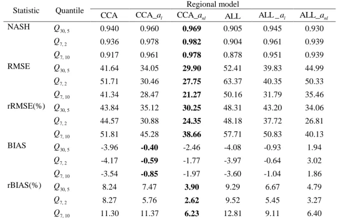
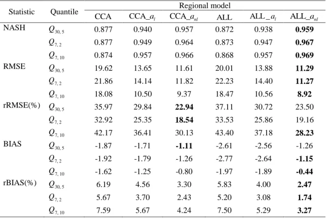
Tables 2 and 3 present the performance indices obtained for the different regional models for 302
summer and winter low-flow quantile estimation respectively. Results show that adding a 303
recession variable to a regression model always improves significantly the performances. In 304
general, better performances are obtained with regression models including a instead of nl a . l 305
For instance, lower rRMSE and rBIAS are always obtained with a instead of nl a . On the l 306
other hand, for the summer season, better RMSE and NASH are obtained for ALL_a l
307
compared to ALL_a . Results show also that, in general, the delineation of neighbourhoods nl
308
with CCA improves the performances for summer quantiles. This is not the case for winter 309
15
quantiles where performances are generally very similar. This seems to indicate that the 310
overall level of homogeneity in the study region is higher for winter low-flows. Overall best 311
performances are obtained with the model CCA_a for the summer season and with nl 312
ALL_a and CCA_nl a for the winter season. nl 313
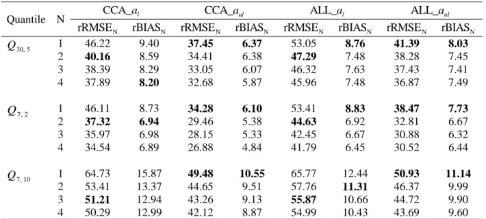
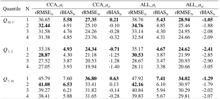
Results in Tables 2 and 3 are obtained under the assumption that the recession variable is 314
available at the target site. In real world cases, the target site is often either ungaged or 315
partially gaged. These results represent a sort of upper bound in terms of regional model 316
performance. Tables 4 and 5 present the performances that are obtained for the simulated 317
partially gaged case. They present the indices rRMSE and N rBIAS for the regional models N 318
when the recession variables at target sites are estimated using a given number N of years. 319
Results indicate that the rRMSE decreases as N increases and converges to the value N 320
obtained with the completely gaged cases for both seasons (see Tables 2 and 3). rBIAS N 321
generally decreases as N increases but occasionally increases instead. This occurs more often 322
for winter quantiles with CCA_a and ALL_nl a , although the biases are small in this cases. nl 323
To assess the improvements obtained by the use of a recession parameter at partially gaged 324
stations, performances of models that include a recession variable (CCA_a , CCA_l a , nl 325
ALL_a and ALL_l a ) are compared to the performances obtained by their corresponding nl 326
ungaged models (CCA or ALL ). For instance, CCA_a is compared with nl CCA. When a nl 327
is included in the model, rRMSE and N rBIAS are always better than the ungaged case even N 328
when only one year of stramflow data (N=1) is used. On the other side, when a is included l 329
in the model, more years are required to lead to better performances than the ungaged case. 330
Thus, in general, two years are required to obtain a better rRMSE for both seasons. To N 331
16
obtain improved rBIAS , generally 1 or 2 years are required for both seasons. However, for N 332
CCA_a and the summer season, 4 years are required for l Q30, 5 and more than 4 years are 333
required for Q7, 10. These results indicate clearly that it is beneficial to use recession 334
parameters at partially gaged sites in a regional low-flow frequency analysis model. Indeed, 335
quantile estimates are improved even when recession parameters are estimated based on a 336
very limited number of years of streamflow data. These results show also the importance of 337
using the non-linear model instead of the linear one as the performances are improved 338
significantly even with only one year of streamflow data compared to the ungaged case. 339
340
6. Conclusions and future work
341
In this paper, regional low-flow frequency analysis models that include recession 342
parameters as predictors are developed. Two different parameters are considered: the 343
recession coefficient a assuming the linear reservoir model and the recession coefficient l a nl 344
assuming a non-linear reservoir model where the exponent b is fixed to the estimated value of 345
1.66 for the study area. 346
The investigation of the appropriate predictors for low-flow statistics is carried out with 347
stepwise regression analysis and leads to the conclusion that the variables from recession 348
parameters are important explanatory variables. The study results clearly indicate that the 349
inclusion of a recession variable in a regional low-flow frequency analysis model improves 350
the performance of the regional estimator. Furthermore, the performances are significantly 351
better with models that include a recession variable from the non-linear reservoir model. 352
17
An inconvenience of using recession characteristics is that they can only be obtained for 353
gaged catchments. However, it is possible to estimate these parameters with a limited number 354
of hydrographs. This paper aims also to evaluate the performances obtained with recession 355
parameters estimated from very short streamflow records. Results of the application of 356
regional low-flow frequency models with hydrograph lengths ranging from 1 to 4 years show 357
that performances converge rapidly to those obtained when the parameters are estimated from 358
the complete data record. When the parameter from the non-linear model is included in a 359
regression model, the performances are better than those obtained without recession variable 360
even when only one year of streamflow data is used to estimate the recession parameter. This 361
shows the possibility of combining local hydrological information with regional information 362
at a partially gaged site in a regional model. 363
These results indicate that it is of interest to dedicate efforts to the development of improved 364
methods for the estimation of recession parameters. Improvements can result principally from 365
the selection of a proper reservoir model and from the recession analysis method. Better 366
reservoir models, in agreement with the real reservoir storage-outflow relationship should be 367
developed. Improved reservoir models, such as the ones that consider various loss and gain 368
sources that affect the streamflow could be used. 369
Other improvements can result from the development of enhanced recession analysis 370
methods. For instance, recession segments should be representative of baseflow recession 371
discharges, i.e. should represent portions of flow that are free of surface flow and interflow. 372
Stoelzle et al. (2013) compared three different methods for the extraction of recessions and 373
three methods for model fitting. They concluded that the roles of recession extraction 374
procedures and fitting methods for the parameterization of storage–outflow models are 375
complex. They also indicated that the interaction of the recession analysis components has 376
18
various effects on the derived recession characteristics. These conclusions imply that the 377
results obtained here are strongly associated to the specific recession analysis method used. 378
Future research efforts should focus on the identification of the recession analysis methods 379
that are the best adapted to low flow regionalization. 380
Other methods for the delineation of homogenous regions should also be considered. For 381
instance, methods based on seasonality characteristics should be very promising (See 382
Cunderlik et al., 2004a, 2004b; Ouarda et al., 2006). Future efforts should also focus on 383
improved modeling of the homogeneity of delineated regions and on the adoption of the 384
multivariate framework (Chebana and Ouarda, 2007, 2008, 2009) for the regional analysis of 385
low-flow characteristics. 386
19
References
388
Arihood, L.D., Glatfelter, D.R., 1991. Method for estimating low-flow characteristics of 389
ungaged streams in Indiana. USGS Water Supply Paper 2372, 22 pp. 390
Bingham, R.H., 1986. Regionalization of low-flow characteristics of Tennessee streams. 391
Water-Resources Investigations Report 85-4191, 63 pp. 392
Boussinesq, J., 1877. Essai sur la théorie des eaux courantes, Du mouvement non permanent 393
des eaux souterraines, Acad. Sci. Inst. Fr. 23, 252-260. 394
Brutsaert, W., Lopez, J.P., 1998. Basin-scale geohydrologic drought flow features of riparian 395
aquifers in the Southern Great Plains. Water Resources Research 34(2), 233-240. 396
Brutsaert, W., Nieber, J.L., 1977. Regionalized drought flow hydrographs from a mature 397
glaciated plateau. Water Resources Research 13(3), 637-643. 398
Chapman, T., 1999. A comparison of algorithms for stream flow recession and baseflow 399
separation. Hydrological Processes 13(5), 701-714. 400
Chapman, T.G., 2003. Modelling stream recession flows. Environmental Modelling & 401
Software 18(8–9), 683-692. 402
Chebana, F., Ouarda, T.B.J.M., 2007. Multivariate L-moment homogeneity test. Water 403
Resources Research 43(8), W08406. 404
Chebana, F., Ouarda, T.B.M.J., 2008. Depth and homogeneity in regional flood frequency 405
analysis. Water Resources Research 44, W11422. 406
20
Chebana, F., Ouarda, T.B.J.M., 2009. Index flood–based multivariate regional frequency 407
analysis. Water Resources Research 45, W10435. 408
Cunderlik, J.M., Ouarda, T., Bobée, B., 2004a. Determination of flood seasonality from 409
hydrological records. Hydrological Sciences Journal-Journal Des Sciences 410
Hydrologiques 49(3), 511-526. 411
Cunderlik, J.M., Ouarda, T.B.M.J., Bobée, B., 2004b. On the objective identification of flood 412
seasons. Water Resources Research 40(1), W01520. 413
Demuth, S., Hagemann, I., 1994. Estimation of flow parameters applying hydrogeological 414
area information. IAHS Publications 221, 151-157. 415
Durrans, S., Ouarda, T., Rasmussen, P., Bobée, B., 1999. Treatment of Zeroes in Tail 416
Modeling of Low Flows. Journal of Hydrologic Engineering 4(1), 19-27. 417
Eng, K., Milly, P.C.D., 2007. Relating low-flow characteristics to the base flow recession 418
time constant at partial record stream gauges. Water Resources Research 43(1), 419
W01201. 420
Fiala, T., Ouarda, T.B.M.J., Hladný, J., 2010. Evolution of low flows in the Czech Republic. 421
Journal of Hydrology 393(3–4), 206-218. 422
Hamza, A., Ouarda, T.B.M.J., Durrans, S.R., Bobée, B., 2001. Développement de modèles de 423
queues et d'invariance d'échelle pour l'estimation régionale des débits d'étiage. 424
Canadian Journal of Civil Engineering 28(2), 291-304. 425
21
Khalil, B., Ouarda, T.B.M.J., St-Hilaire, A., 2011. Estimation of water quality characteristics 426
at ungauged sites using artificial neural networks and canonical correlation analysis. 427
Journal of Hydrology 405(3–4), 277-287. 428
Khaliq, M.N., Ouarda, T.B.M.J., Gachon, P., 2009. Identification of temporal trends in annual 429
and seasonal low flows occurring in Canadian rivers: The effect of short- and long-430
term persistence. Journal of Hydrology 369(1-2), 183-197. 431
Khaliq, M.N., Ouarda, T.B.M.J., Gachon, P., Sushama, L., 2008. Temporal evolution of low-432
flow regimes in Canadian rivers. Water Resources Research 44(8), W08436. 433
Kroll, C.N., Luz, J.G., Allen, T.B., Vogel, R.M., 2004. Developing a watershed 434
characteristics database to improve low streamflow prediction. Journal of Hydrologic 435
Engineering, ASCE 9(2), 116-125. 436
Moore, R.D., 1997. Storage-outflow modelling of streamflow recessions, with application to a 437
shallow-soil forested catchment. Journal of Hydrology 198(1–4), 260-270. 438
Nathan, R.J., McMahon, T.A., 1990. Identification of homogeneous regions for the purposes 439
of regionalisation. Journal of Hydrology 121(1–4), 217-238. 440
Ouarda, T.B.M.J., Jourdain, V., Gignac, N., Gingras, H., Herrera, E., Bobée, B., 2005. 441
Développement d'un modèle hydrologique visant l'estimation des débits d'étiage pour 442
le Québec habité. INRS-ETE, Rapport de recherche No. R-684-f1, 174 pp. 443
Ouarda, T.B.M.J., Ba, K.M., Diaz-Delgado, C., Carsteanu, A., Chokmani, K., Gingras, H., 444
Quentin, E., Trujillo, E., Bobée, B., 2008a. Intercomparison of regional flood 445
22
frequency estimation methods at ungauged sites for a Mexican case study. Journal of 446
Hydrology 348(1-2), 40-58. 447
Ouarda, T.B.M.J., Charron, C., St-Hilaire, A., 2008b. Statistical Models and the Estimation of 448
Low Flows. Canadian Water Resources Journal 33(2), 195-206. 449
Ouarda, T.B.M.J., Cunderlik, J.M., St-Hilaire, A., Barbet, M., Bruneau, P., Bobée, B., 2006. 450
Data-based comparison of seasonality-based regional flood frequency methods. 451
Journal of Hydrology 330(1-2), 329-339. 452
Ouarda, T.B.M.J., Girard, C., Cavadias, G.S., Bobée, B., 2001. Regional flood frequency 453
estimation with canonical correlation analysis. Journal of Hydrology 254(1-4), 157-454
173. 455
Ouarda, T.B.M.J., Haché, M., Bruneau, P., Bobée, B., 2000. Regional flood peak and volume 456
estimation in northern Canadian basin. Journal of cold regions engineering 14(4), 176-457
191. 458
Ouarda, T.B.M.J., Shu, C., 2009. Regional low-flow frequency analysis using single and 459
ensemble artificial neural networks. Water Resources Research 45(11), W11428. 460
Smakhtin, V.U., 2001. Low flow hydrology: a review. Journal of Hydrology 240(3–4), 147-461
186. 462
Stoelzle, M., Stahl, K., Weiler, M., 2013. Are streamflow recession characteristics really 463
characteristic? Hydrology and Earth System Sciences 17(2), 817-828. 464
Tallaksen, L.M., 1989. Analysis of time variability in recession. IAHS Publications 187, 85-465
96. 466
23
Tallaksen, L.M., 1995. A review of baseflow recession analysis. Journal of Hydrology 165(1– 467
4), 349-370. 468
Tsakiris, G., Nalbantis, I., Cavadias, G., 2011. Regionalization of low flows based on 469
Canonical Correlation Analysis. Advances in Water Resources 34(7), 865-872. 470
Vogel, R.M., Kroll, C.N., 1992. Regional geohydrologic-geomorphic relationships for the 471
estimation of low-flow statistics. Water Resources Research 28(9), 2451-2458. 472
Vogel, R.M., Kroll, C.N., 1996. Estimation of baseflow recession constants. Water Resources 473
Management 10(4), 303-320. 474
Wittenberg, H., 1994. Nonlinear analysis of flow recession curves. IAHS Publication 221, 61-475
67. 476
Wittenberg, H., 1999. Baseflow recession and recharge as nonlinear storage processes. 477
Hydrological Processes 13(5), 715-726. 478
24
Table 1. Explanatory variables available for the study area. 480
Explanatory variable Units Notation
Drainage area km2 AREA
Mean slope of the drainage area degree MSLP
Percentage of forested area % PFOR
Percentage of lakes % PLAKE
Mean annual precipitation mm PTMA
Mean summer-fall precipitation mm PLMS
Mean annual degree-days < 0 ºC degree day DDBZ
Mean annual degree-days > 13 ºC degree day DDH13
Number of days where temperatures > 27 ºC day NDH27
Mean curve number - MCN
Latitude of the gaging station degree LAT
Recession parameter (linear case, b=1) s-1 al
Recession parameter (non-linear case, b=bopt) m3(1-b)sb-2 anl
481 482 483 484 485
25
Table 2. Performances of regional models for summer low-flow quantile estimation. 486
Statistic Quantile Regional model
CCA CCA_a l CCA_a nl ALL ALL _a l ALL_a nl
NASH Q30, 5 0.940 0.960 0.969 0.905 0.945 0.930 7, 2 Q 0.936 0.978 0.982 0.904 0.961 0.939 7, 10 Q 0.917 0.961 0.978 0.878 0.951 0.939 RMSE Q30, 5 41.64 34.05 29.90 52.41 39.83 44.99 7, 2 Q 51.71 30.46 27.75 63.37 40.35 50.33 7, 10 Q 41.34 28.47 21.27 50.16 31.79 35.46 rRMSE(%) Q30, 5 43.84 35.12 30.25 48.31 43.20 34.06 7, 2 Q 44.57 30.88 24.35 48.18 37.72 26.81 7, 10 Q 51.81 45.28 38.66 57.71 50.83 40.13 BIAS Q30, 5 -3.96 -0.40 -2.46 -4.08 -0.93 1.94 7, 2 Q -4.17 -0.59 -1.77 -3.97 -0.64 3.02 7, 10 Q -3.54 -0.85 -1.97 -3.60 -1.04 1.86 rBIAS(%) Q30, 5 8.24 7.47 3.90 9.29 6.67 4.79 7, 2 Q 8.27 5.76 2.62 9.52 5.45 3.27 7, 10 Q 11.30 11.37 6.23 12.81 9.11 6.40
Bold values correspond to best performances.
487 488 489
26
Table 3. Performances of regional models for winter low-flow quantile estimation. 490
Statistic Quantile Regional model
CCA CCA_a l CCA_a nl ALL ALL _a l ALL_a nl
NASH Q30, 5 0.877 0.940 0.957 0.872 0.938 0.959 7, 2 Q 0.877 0.949 0.964 0.873 0.947 0.967 7, 10 Q 0.874 0.957 0.966 0.868 0.957 0.969 RMSE Q30, 5 19.62 13.65 11.61 20.01 13.88 11.29 7, 2 Q 21.86 14.14 11.82 22.23 14.40 11.27 7, 10 Q 18.08 10.50 9.37 18.47 10.56 8.92 rRMSE(%) Q30, 5 35.97 29.84 22.94 37.11 30.72 23.50 7, 2 Q 32.92 25.35 18.54 33.53 25.86 19.16 7, 10 Q 42.17 36.41 30.13 43.40 37.18 28.23 BIAS Q30, 5 -1.87 -1.71 -1.11 -2.61 -2.56 -1.26 7, 2 Q -1.92 -1.79 -1.26 -2.77 -2.64 -1.15 7, 10 Q -1.62 -1.25 -0.80 -1.97 -1.89 -0.44 rBIAS(%) Q30, 5 6.19 4.56 3.30 5.83 4.00 2.47 7, 2 Q 5.67 3.70 2.43 5.20 3.08 1.74 7, 10 Q 7.59 5.67 4.24 7.50 5.29 3.27
Bold values correspond to best performances.
491 492 493
27
Table 4. Performances of regional models for partially gaged basins (Summer low-flow 494
quantile estimation). 495
Quantile N CCA_a l CCA_a nl ALL_a l ALL_a nl
N
rRMSE rBIAS N rRMSE N rBIAS N rRMSE N rBIAS N rRMSE N rBIAS N
30, 5 Q 1 46.22 9.40 37.45 6.37 53.05 8.76 41.39 8.03 2 40.16 8.59 34.41 6.38 47.29 7.48 38.28 7.45 3 38.39 8.29 33.05 6.07 46.32 7.63 37.43 7.41 4 37.89 8.20 32.68 5.87 45.96 7.48 36.87 7.49 7, 2 Q 1 46.11 8.73 34.28 6.10 53.41 8.83 38.47 7.73 2 37.32 6.94 29.46 5.38 44.63 6.92 32.81 6.67 3 35.97 6.98 28.15 5.33 42.45 6.67 30.88 6.32 4 34.54 6.89 26.88 4.84 41.79 6.45 30.52 6.44 7, 10 Q 1 64.73 15.87 49.48 10.55 65.77 12.44 50.93 11.14 2 53.41 13.37 44.65 9.51 57.76 11.31 46.37 9.99 3 51.21 12.94 43.26 9.13 55.87 10.66 44.72 9.90 4 50.29 12.99 42.12 8.87 54.99 10.43 43.69 9.60
Bold values correspond to performances surpassing the corresponding ungaged case model. 496
28
Table 5. Performances of regional models for partially gaged basins (Winter low-flow 498
quantile estimation). 499
Quantile N CCA_a l CCA_a nl ALL_a l ALL_a nl
N
rRMSE rBIAS N rRMSE N rBIAS N rRMSE N rBIAS N rRMSE N rBIAS N
30, 5 Q 1 36.65 5.58 27.35 0.21 38.76 5.43 28.94 -1.05 2 32.44 4.91 25.10 -0.10 34.76 4.85 25.46 -1.88 3 31.58 4.76 24.26 -0.28 33.14 4.30 24.95 -2.08 4 31.38 4.85 23.76 -0.32 32.54 4.31 24.66 -2.09 7, 2 Q 1 33.18 4.93 24.34 -0.71 35.17 4.67 24.62 -2.41 2 28.87 4.30 21.18 -1.25 30.53 3.87 21.99 -2.85 3 27.52 3.87 20.53 -1.28 28.67 3.47 20.93 -2.90 4 27.05 3.93 19.94 -1.40 28.11 3.38 20.66 -3.05 7, 10 Q 1 45.79 7.60 36.80 0.63 47.92 7.41 34.02 -1.29 2 41.08 6.53 33.41 0.13 42.16 6.10 30.97 -1.79 3 39.27 6.21 31.82 -0.14 40.84 5.94 30.29 -2.02 4 38.41 5.88 31.65 -0.28 39.83 5.67 29.81 -2.07
Bold values correspond to performances surpassing the corresponding ungaged case model. 500
501
29
Figure captions
503
Figure 1. Hydrometric stations of the study area. 504
Figure 2. Normal probability plot for the station 023402. 505
Figure 3. Streamflow for the year 1970 at station 020802. Recession segments are identified 506
with grey areas. 507
Figure 4. Plot of –dQ/dt versus Q for the station 030103. 508
30 510 511 Figure 1. 512 513
31 514
Figure 2. 515
32 517 518 Figure 3. 519 520
33 521 522 Figure 4. 523 524