a publisher's https://oatao.univ-toulouse.fr/26990
https://doi.org/10.1029/2019JE006278
Garcia, Raphaël F. and Kenda, Balthasar and Kawamura, Taichi and Spiga, Aymeric and Murdoch, Naomi and Lognonné, Philippe and Widmer͈Schnidrig, Ruldolf and Compaire, Nicolas and Orhand͈Mainsant, GuÏnolÏ and Banfield, Donald and Banerdt, William Bruce Pressure Effects on the SEIS͈InSight Instrument, Improvement of Seismic Records, and Characterization of Long Period Atmospheric Waves From Ground Displacements. (2020) Journal of Geophysical Research: Planets, 125 (7). ISSN 2169-9097
SEIS seismometer (Lognonné et al., 2020) demonstrated that the main noise sources are indeed coming from Mars' atmosphere activity. Similar to a seismometer situated on the ocean floor (Crawford et al., 1991), an important source of signal on the seismometer is due to elastic ground deformations induced by variations of the atmospheric pressure. This signal can be removed by using pressure measurements (Beauduin et al., 1996; Crawford, 2000; Zürn et al., 2007; Zürn & Widmer, 1995). In addition, the relations between seismic and pressure records allow the subsurface mechanical properties to be estimated (Tanimoto & Wang, 2019) and constraints to be placed on atmosphere or ocean dynamics.
In the following, we first describe the instrument noise and data characteristics of the pressure and seismic sensors, including the coherence between the pressure and seismic records. Then we present two differ-ent methods to remove the ground displacemdiffer-ent signal generated by atmospheric pressure variations from seismic records. The results of these two methods are compared, and the improvement of seismic records is quantified. As a side product of these two methods, estimates of frequency-dependent compliance val-ues (ratio of ground velocity to pressure) are presented. Finally, we consider the use of seismological data to constrain the atmospheric dynamics. We suggest that this is a valuable complement to measurements by InSight's weather station (Banfield et al., 2019), in particular for large amplitude signals recorded by the pressure sensor and putatively attributed to atmospheric gravity waves. We conclude on the interest of these methods for seismic signal detection and analysis.
2. Pressure and Seismic Data Sets
2.1. Pressure and Broad-Band Seismic Sensors and Instrument Noise
The SEIS (Seismic Experiment for Internal Structure of Mars) instrument is the core instrument of InSight mission (Lognonné et al., 2019). It is composed of six seismic sensors: three Short Period (SP) sensors and three Very Broad Band (VBB) sensors, all of them presenting an instrument noise level below their require-ments. Only the VBB sensors are considered in this study as their noise levels are lower than the SP sensors' noise levels for frequencies <≈5 Hz. Each of the VBB sensors produces two different channels: a velocity channel (VEL) with best performances at frequencies higher than 0.02 Hz and a position channel (POS) with best performances at frequencies lower than 0.1 Hz. SEIS VBB velocity data at 2 samples per seconds (sps) and SEIS VBB position data at 0.5 sps have been used in this study (Insight Mars SEIS Data Service, 2019). Corresponding channel names are indicated by SEED (Standard for the Exchange of Earthquake Data) “location.name” codes “02.MH” and “00.VM,” respectively, for the SEIS velocity and position channels. The following data pre-processing steps have been applied to the VBB data:
• removal of the 1 s period tick noise induced by contamination from SEIS temperature measurements. This noise has a small amplitude (below 40 counts peak to peak amplitude) and can be easily removed due to its very regular shape repeating every second.
• removal of glitch patterns, induced by various instantaneous mechanical relaxations at the sensor or instrument level, that have the shape of the instrument response to a step in acceleration. The principle of the glitch removal method is described in Lognonné et al. (2020).
• removal of the seismic sensors' transfer functions according to the metadata documented in the dataless SEED volume.
• rotation into the vertical (Z), North-South (N or NS), and East-West (E or EW) geographical reference frame of the ground velocity records.
The Auxiliary Payload Sensor Suite (APSS) is a set of three instruments implemented on the InSight mission to monitor the Martian weather and magnetic environments in order to correct for the ground displacements induced by the atmosphere dynamics and any instrument noise generated by the residual magnetic sensi-tivity of VBB sensors (Banfield et al., 2019). It is composed of a three-axis fluxgate magnetometer (MAG), a wind sensor (TWINS) providing horizontal wind speed and incoming direction, and a pressure sensor. The pressure sensor considered in this study has a sampling rate (up to 20 sps) and a noise level of unprecedented quality on the surface of Mars. Calibrated pressure data at 2 sps in Pascal unit are used in this study. These channels have the SEED “location.name” code “13.MDO.” These data are calibrated by the APSS instrument team by using output voltage and sensor temperature channel (Banfield et al., 2019).
The pressure and wind sensors are located on the lander deck at a height of approximately 1.2 m. The SEIS instrument is located on the ground, at approximately 1.6 m from the edge of the lander deck, and at an Software: Raphael F. Garcia,
Balthasar Kenda, Nicolas Compaire Validation: Raphael F. Garcia Writing - Original Draft: Raphael F. Garcia
Investigation: Aymeric Spiga, Naomi Murdoch
Project Administration: Raphael F. Garcia, Donald Banfield Resources: Donald Banfield Supervision: William Bruce Banerdt Writing - review & editing: Balthasar Kenda, Aymeric Spiga, Naomi Murdoch,
Journal of Geophysical Research: Planets
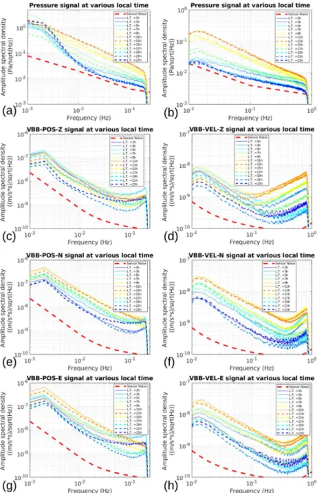
10.1029/2019JE006278Figure 1. Amplitude spectral densities of Pressure records (a, b), and SEIS VBB-POS (on the left) and VBB-VEL (on the
right) records of vertical (c, d), NS (e, f), and EW (g, h) components averaged over 2 hr local time windows. Signals are provided in the 1–250 mHz range on the left and in the 0.01–1 Hz range on the right. The center of the local time window in hours is indicated in the legend. Continuous data from 1 April 2019 to 25 April 2019 (sols 123 to 146) have been used to compute these curves. The reduction of power below 0.002 Hz on the left panels and below 0.015 Hz on the right panels is due to filtering. It is not present in the raw data.
azimuth of about 190◦from the lander center of figure. SEIS is protected against any direct effects of wind
and sun illumination by its wind and thermal shield.
2.2. Daily Variability of Pressure and Seismic Records
The daily variability of pressure and seismic records is illustrated in Figure 1 by computing Amplitude Spec-tral Densities (ASD) averaged over 2 hr periods at various local times. The amplitude of the signals recorded on these two instruments clearly varies with local time with the highest energy at midday and the lowest
after sunset to 2 a.m. Local Mean Solar Time (LMST). This trend is due to atmospheric activity which is pre-dicted to be much more energetic during day than during night, owing to turbulent convection in the day time (Spiga et al., 2018). Note, however, that morning hours before sunrise (2–6 a.m. LMST) present energy levels in between the two extreme values, due to high winds in this time period which generate shear-driven turbulence.
The pressure signals are shown in Figures 1a and 1b for two different frequency ranges. More energy is visible during the day at frequencies above 0.01 Hz. However, an increase of pressure energy is clearly observed below 0.04 Hz, in particular during the night time, which is attributed to gravity wave activity (Banfield et al., 2019; Spiga et al., 2018). Above 0.01 Hz, during the periods of lowest signal (6 p.m. to 2 a.m. LMST), the ASD curves gather on a single line slightly above the theoretical noise level. This observation suggests that during these times of the Martian sol the pressure sensor is measuring signals close to its instrumental noise. The SEIS-VBB channels present a pattern with two slopes crossing in the 0.1–0.5 Hz range. This background signal and its variation during a Martian sol is in good agreement with the noise model of the instrument established before the launch of the mission (Mimoun et al., 2017). The low frequency signals on the hori-zontal components are mainly due to ground tilts projecting the Martian gravity in the horihori-zontal sensing direction of SEIS. These ground rotations are generated by both the lander vibrations induced by the wind drag force (Murdoch et al., 2017) and the surface pressure variations induced by atmospheric dynamics (Kenda et al., 2017; Lorenz et al., 2015; Murdoch et al., 2017). On the SEIS vertical channel, the low frequency background signal is generated by a combination of residual temperature sensitivity (Mimoun et al., 2017), pressure variations (Kenda et al., 2017; Murdoch et al., 2017), and wind shear stress effects acting directly on the ground. The proportion of these various contributions is not currently quantified at the time of this study. However, both the thermal noise and pressure noise are predicted to be below 10−9m∕s∕s∕√Hz for
frequencies above 0.01 Hz for the vertical component. On the other hand, a high noise level is observed on the vertical component in the 0.01–0.1 Hz frequency range during the 2 a.m. to 6 a.m. period. As this time period is dominated by a constant laminar wind with a stable vertical gradient in a cold and dense atmosphere, this observation suggests that wind shear stress applied to the ground surface is a significant contributor to the noise. However, we cannot discriminate between wind variations induced by a thin layer of viscous interactions close to the surface or by turbulence in a thicker layer Petrosyan et al. (2011). At high frequencies, the background signals are interpreted as the effect of ground deformations due to lander vibra-tions induced by the wind drag force. The amplitude of the noise below and above 0.1 Hz is proportional to the wind amplitude and wind amplitude squared, respectively, while the noise floor at 0.1 Hz is close to the sensor Brownian noise. As predicted by Murdoch et al. (2017), the wind-driven lander noise above 0.1 Hz is larger on the vertical than on the horizontal components. In summary, as expected from the SEIS noise model and demonstrated below, the wind noise dominates the background SEIS signals (see first supple-mentary material of Lognonné et al., 2020). The pressure noise dominates only when pressure variations are large in amplitude (>≈0.2 Pa, see section 4). In addition, the assumptions underlying the compliance theory (see section 2.4), and more detailed computations performed for the pressure drops created by dust devils (Murdoch et al., 2017), indicate that ground deformations will be significant only for pressure variations that are coherent over large horizontal scales (>≈20 m).
2.3. Coherence Between Pressure and Seismic Records
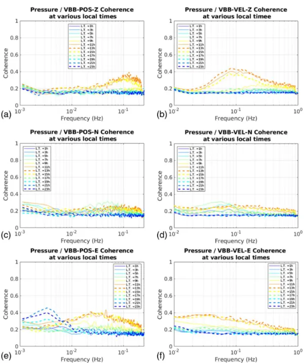
The coherence between SEIS-VBB channels and the pressure sensor is investigated here by using two dif-ferent representations. The first one presented in Figure 2 is showing average values of coherence between pressure and SEIS components, computed, respectively, in 60 and 15 min windows for POS and VEL chan-nels, at various local times. These data suggest that SEIS vertical and horizontal components present coherences with pressure in the 10 a.m. to 4 p.m. local time range and in different frequency bands, which suggest that during that time, the pressure is a significant source of noise. The frequency range has an upper limit of 1 Hz because no correlation between the pressure and SEIS components was detected above 1 Hz. The vertical component is mainly coherent with pressure in the 0.03–0.5 Hz frequency range because this coherence is limited for lower and higher frequencies by the SEIS noise sources described above. The NS component presents lower coherence with pressure than the EW component. A combination of effects can explain this feature. First, the noise is higher on this component due to residual glitch noise and to other noise sources in this direction pointing toward the lander. The tilt signals are also smaller due to the wind direction being mainly West-East during this period and possibly also due to a lower compliance value in
Journal of Geophysical Research: Planets
10.1029/2019JE006278Figure 2. Coherence between Pressure and SEIS VBB-POS (on the left) and VBB-VEL (on the right) for vertical (a, b), NS (c, d), and EW (e, f) components,
computed over 60 and 15 min windows, respectively, for POS and VEL channels, and averaged over 2 hr local time windows. The center of the local time window in hours is indicated in the legend. Continuous data at 2 sps from 1 April 2019 to 25 April 2019 (sols 123 to 146) have been used to compute these curves.
this direction (see section 4.3). The coherence with the horizontal components also decreases strongly above 0.5 Hz due to the wind-induced noise on SEIS sensors. However, during the day time period considered here, the coherence with the EW component extends to frequencies lower than 0.01 Hz due to compliance effects generated by tilts, as described below. During the night time the overall coherence between the pres-sure and SEIS components is weak because of weak prespres-sure variations. However, a noticeable exception is a significant average coherence increase for EW components in the 1–7 mHz range during evening hours (6 p.m. to midnight LMST) due to ground movements generated by atmospheric gravity waves (Spiga et al., 2018, section 5.2.3). The presence of this signal only on the EW component indicates a relation with either the background wind or the gravity wave propagation direction.
Figure 3. On top (a): Pressure variations (in Pa) of sols 82 and 83, band pass filtered between 1 and 600 s periods. On the bottom (b): coherograms (coherence as
function of time and frequency) between pressure and SEIS vertical (top panel), NS (middle panel), and EW (bottom panel) components. Frequency, along the y axis in log scale, ranges from 0.01 to 1 Hz. Time, along the x axis, is expressed in LMST hours. Coherence is provided as a color scale.
The analyses of average coherence made above hide the fact that the coherence between SEIS and the pres-sure sensor is varying on time scales smaller than the 60 and 15 min windows used for averaging. To illustrate this, Figure 3 presents coherograms (coherence as a function of time and frequency) during two sols. The pressure variations present large pressure drops due to convective vortices that are generating large coher-ent signals on the SEIS sensors during day time (Kenda et al., 2017; Spiga et al., 2018, sections 2.3 and 5.2.2). Some coherence between the pressure and EW component is also visible at the end of sol 82 at low frequen-cies, possibly related to gravity wave activity. Outside of these events, the pressure variations are smaller, thus inducing signals on SEIS sensors that fall below the amplitude of the wind-generated noise. The coherogram pattern is significantly different between the NS and EW components because the ground tilt directions depend on the direction of atmospheric wind that changes over the sol. During this time period, the wind is along the North/South direction only during early morning hours.
2.4. Compliance Theory and Noise Limitations
The ground deformations generated by atmospheric pressure variations induce various effects on the components of the SEIS instrument:
Journal of Geophysical Research: Planets
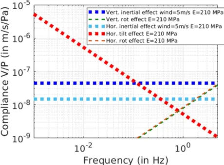
10.1029/2019JE006278Figure 4. Theoretical prediction by Sorrells' theory of the ground Velocity over Pressure ratio (V/P in m/s/Pa) as a
function of frequency (in Hz) for the vertical and horizontal components of ground velocity and for the three types of effects described in this section. Pressure perturbations are assumed to move horizontally with a wind speed of 5 m/s, and VBB sensor positions relative to SEIS center of mass given by Fayon et al. (2018) are taken into account.
• Inertial effects. An harmonic pressure wave propagating horizontally over the ground will lead to vertical and horizontal surface displacements due to the continuity of stress and vertical displacement at the sur-face (Sorrells, 1971). These are sensed by SEIS as inertial effects that can be computed with a quasi-static approximation (Sorrells, 1971). For a given frequency these accelerations are proportional to the hori-zontal speed at which the pressure perturbation is moving. Hence, the ratio V/P (ground Velocity V over Pressure P) does not depend on frequency for an homogeneous subsurface and generally increases with frequency for subsurface models that have increasing rigidity with depth.
• Tilt effects. An harmonic pressure wave propagating over the ground will also lead to a local tilting of the free surface on which SEIS is installed. Because of this tilt the Martian gravity vector is projected onto the horizontal components leading to a static acceleration signal proportional to the tilt. For an homogeneous subsurface, this tilt is independent of the horizontal speed at which the pressure perturbation is moving, and it is proportional to an acceleration. Therefore, the ratio V/P decreases with increasing frequency. • Rotation effects. Like short period seismic waves Fayon et al. (2018), a short wavelength pressure-induced
tilt of the ground leads also to a rotation of SEIS around the geometrical center of its feet. This effect depends on the position of the individual VBB sensors relative to the geometrical center of SEIS feet, and, for an homogeneous subsurface, it is independent of the horizontal speed at which the pressure pertur-bation is moving. However, the effect is proportional to displacement, and thus, the ratio V/P increases with increasing frequency.
• Free air anomaly. At longer periods and below the seismic bandwidth, the vertical inertial acceleration is smaller than the free air gravity correction for angular frequencies smaller than 2 g∕r, where g and r are the Martian gravity and radius (Lognonné & Clévédé, 2002). Given that this effect is significant only below about 0.24 mHz, it is neglected here.
We consider these effects as static and local elastic ground deformations and neglect both the inertia and their propagation. They are theoretically described either by assuming that the pressure perturbations are plane waves moving in the wind direction (Kenda et al., 2017; Sorrells, 1971) or by estimating the negative load of a given convective vortex and assuming that it follows a simple straight line trajectory (close to the background wind direction) (Banerdt et al., 2020; Lorenz et al., 2015). A summary of Sorrells' theory for an homogeneous subsurface model is provided in Figure 4. Assuming an arbitrary homogeneous subsurface model described by a Young modulus of 210 MPa and a Poisson's ratio of 0.25, the ratios between vertical
and horizontal ground velocities (measured by SEIS) and the pressure variations are predicted. Under the homogeneous subsurface assumption, and assuming the pressure perturbations are plane waves, the various compliance effects have the following forms for the vertical (Vz) and horizontal along wave vector (VH) ground velocities under a pressure perturbation (P):
• Inertial effects:VZ P = − ic(𝜆+2𝜇) 2𝜇(𝜆+𝜇)and VH P = − c 2𝜇(𝜆+𝜇) • Tilt effects:VH P = g(𝜆+2𝜇) 2𝜔𝜇(𝜆+𝜇) • Rotation effects:VZ P = i𝜔Dscos(𝛼)(− i 2𝜇(𝜆+𝜇))and VH P = i𝜔Dssin(𝛼)(− i 2𝜇(𝜆+𝜇))
In these formulas, 𝜆 and 𝜇 are the Lamé parameters, g is Martian gravity, c and 𝜔 are, respectively, the hori-zontal speed and the pulsation of the plane wave pressure perturbation, i is the imaginary complex number, Dsis the distance between geometrical center of the SEIS feet and the corresponding seismic sensor, and 𝛼 is
the angle between the geometrical center of the feet, the vertical axis, and the sensor position. Tilt effects on the vertical component are neglected. Due to tilt effects, a large compliance is predicted at low frequencies for the SEIS horizontal component along the wind direction. Only frequency-independent inertial effects are expected for the SEIS vertical component below 1 Hz. Rotation effects are predicted to be dominant only for frequencies above 1 Hz and will be neglected in this study. These predictions explain the features observed in Figure 2: (1) The coherence with the pressure signals extends to lower frequencies for the hor-izontal components than for the vertical component, (2) the EW component (dominant wind direction) presents a larger coherence than the NS component, and (3) the coherence with the vertical component is limited to a frequency range in which the SEIS-VBB noise is the lowest. For the slightly more complex non-homogeneous case see Kenda et al. (2017). The subsurface model can be extracted via the inversion of the subsurface structure from compliance measurements (Kenda et al., 2020; Lognonné et al., 2020).
3. Methods for Pressure Noise Removal on Seismic Records
Two different methods of pressure noise removal are presented. They both rely on the compliance theory under the assumption of plane pressure waves moving with, that is, advected by, the wind. This theoretical description provides a relation between the pressure and the vertical and horizontal along wind seismic signals. The transfer function relating these two variables (the compliance) is estimated from the records. Then, using the compliance, SEIS signals predicted from pressure records are subtracted from the SEIS records in order to generate decorrelated records. The two methods described below differ in physical a prioris, ways of estimating the transfer function, the corrected that are components, and the continuity of correction.
3.1. Method 1: Pressure Noise Removal by Adaptive LMS Filtering
Previous pressure noise decorrelation techniques applied to Earth data have used a linear transfer function between the ground velocity and pressure, usually estimated in the frequency domain (Beauduin et al., 1996). The pressure noise decorrelation method presented here relies on the assumption that the pressure (P) and the ground velocity (Vi) of SEIS component i are related by the following linear relation:
Vi(n) = N∕2
∑
k=−N∕2
Ci(k)P(n − k), (1)
where Ciis the compliance acausal FIR filter and N is the number of filter coefficients. The acausality is
introduced to account for the fact that the indentation of the ground due to a moving pressure front will precede the pressure front in the forward looking direction because the ground elastic deformation will be sensed by the seismometer before the arrival of the pressure forcing on the pressure sensor. Thus, for an observer at a fixed location, the ground deforms before the pressure front moves overhead and the local air pressure changes. The filter coefficients are estimated with the adaptive LMS method, which provides continuous evolution of the FIR filter coefficients in order to improve the fit to the data, in a way similar to the least squares fitting used by Murdoch et al. (2017). The following improvements to the usual adaptive LMS method are implemented:
• The FIR filter evolution step size is defined to be proportional to the average coherence between the pressure and corresponding SEIS channel.
Journal of Geophysical Research: Planets
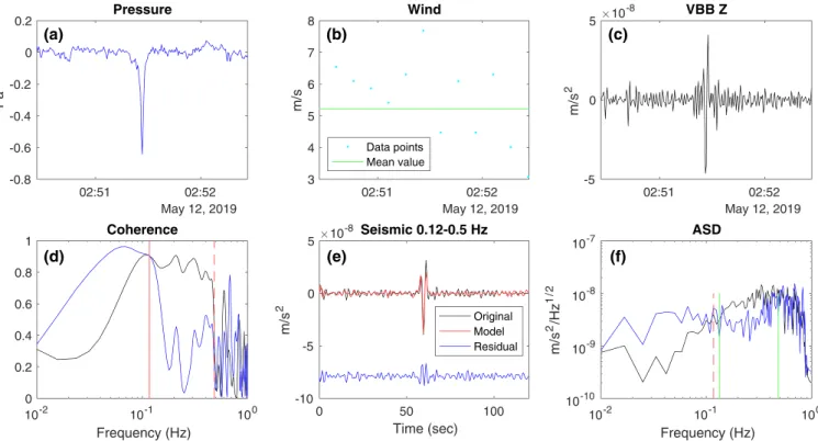
10.1029/2019JE006278Figure 5. Example application of the convective vortices decorrelation method. (a) Detrended pressure time series. (b) Wind speed; the mean value is
calculated after removing the values in correspondence of the vortex encounter. (c) Vertical seismic acceleration as measured by the VBBs (band pass filtered 0.02–1 Hz). (d) Coherence between pressure and seismic signal (black) and residual coherence after removing the best-fitting single-coefficient vortex model (blue, see text). (e) Seismic signal in the frequency band where coherence is lowered by the procedure: the black trace is the original signal, the red trace the modeled signal, and the blue trace the residual signal (shifted). (f) Amplitude spectral density of the original and the residual signal (black and blue curves, respectively); the green lines limit the frequency range where both coherence and amplitude spectral density of the residual are lower; at the central frequency of 0.3 Hz, about 75% of the energy is removed.
• The data are processed in overlapping continuous windows preserving memory of the previous LMS filter estimates.
• The data filtered in various frequency bands are processed, and the signals are recombined after decorrelation.
The filter length is chosen according to the data sampling rate in order to cover a time range of ±100 s. For example, for 2 sps data the filter size is defined as N = 400 − 1. This method does not rely on a priori information coming from the physics of the coupled solid/atmosphere system; however, it has the capability to let the transfer function evolve according to wind direction variations without requiring this information.
3.2. Method 2: Pressure Noise Removal by Modeling of Convective Vortices
A second method is based on the classical Sorrells theory (Sorrells, 1971) stating that the vertical ground velocity Vzis related to the pressure forcing P (measured at the same location) by the relation in the frequency domain:
Vz( 𝑓 ) = ic · Cz( 𝑓 ) · P( 𝑓 ). (2)
In equation (2), i is the imaginary unit, c is the mean wind speed (advecting the pressure fluctuation), and Czis the frequency-dependent compliance. A similar equation holds true for the horizontal component in the direction of the background wind. Prior to the InSight landing on Mars, Murdoch et al. (2017) developed and tested on synthetic data a decorrelation method based on the empirical determination of the compli-ance function Cz. However, the method proves efficient only when the coherence between the seismic and
Figure 6. Efficiency of the LMS decorrelation method tested on data from sols 169 to 174 on VBB-POS (a, c) and VBB-VEL (b, d) channels. (a, b) Amplitude
spectral density of SEIS records before (plain lines) and after (dashed lines) the decorrelation, over the whole time period, for vertical (in red), EW (in blue), and NS (in black) SEIS components. (c, d) ASD improvement (symbols, in %) and number of selected windows (bars) as a function of frequency, for time windows with average coherency larger than 0.5. Color coding is identical to the top panels for the three SEIS components: vertical in red, EW in blue, and NS in black.
during events (i.e., convective vortices), which are of short duration and relatively narrow frequency band. Therefore, equation (2) has been applied to individual events, and, due to their narrow frequency range, with a compliance value not depending on frequency. Thus, a simple proportionality relation is assumed between the pressure and seismic time series for each event, and the apparent compliance Czis computed
by minimizing the misfit between the observed and modeled vertical signals. The latter is then removed from the measured ground velocity, and the algorithm ensures that both the coherence and the Amplitude Spectral Density (ASD) are reduced in the relevant frequency band by the decorrelation process (Figure 5). Note that only the vertical component is considered; indeed, especially in the case of convective vortices, the horizontal tilt effect is more sensitive to the pressure field farther away from the seismometer and is thus not well modeled by this simple approach (Kenda et al., 2017).
4. Results of Pressure Decorrelation Methods
4.1. Efficiency of Pressure Noise Removal Process
The performance of the adaptive LMS decorrelation method is estimated in various ways by comparing decorrelated records to original ones. Before performing the decorrelation process, SEIS VEL channels are downsampled to 2 sps.
The overall improvement in the spectral domain over the whole time period is shown in Figures 6a and 6b. As expected, the improvement is restricted to frequency ranges and components for which the coher-ence with the pressure signal is high. For these average values, the improvement remains below a factor of 2 above 5 mHz, suggesting that the pressure noise is not the dominating noise source. However, POS chan-nels present improvements up to a factor of 4 around 2 mHz, suggesting that in the 1–4 mHz frequency
Journal of Geophysical Research: Planets
10.1029/2019JE006278range the pressure noise dominates. Figures 6c and 6d show the average improvement of background sig-nal amplitude spectral density (in %) only for windows presenting an average coherence larger than 0.5. We retrieve the features already observed in Figure 2, the average coherency being proportional to the num-ber of selected windows in a given frequency range. The average ASD improvements are between 40% and 80% in the frequency ranges where the coherence is significant. The low coherence and pressure decorrela-tion efficiency in the 4–10 mHz range suggest that the wind noise dominates over the pressure noise in this frequency range.
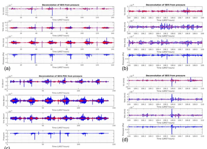
Figure 7 presents the time domain comparison over the sol range 169–174 (Figures 7a and 7c, respectively, for the POS and VEL channels) and zooms on two consecutive hours during the day time active period of sol 173 (Figures 7b and 7d for VEL channels). As shown on these plots, most of the largest pressure signals during the active day time periods generate large SEIS signals. The focus on 1 hr periods demonstrates that the LMS decorrelation method efficiently removes the large convective vortex signals at long period on the horizontal SEIS components. The efficiency is slightly lower for the vertical SEIS component, but still significant. A variability of the apparent compliance resulting from a change of wind direction, different trajectories of the convective vortices, and different wind flows in the vortices is expected. This is observed, for example, in Figures 7b and 7d in which large amplitude convective vortices are generating different ground responses. The efficiency of decorrelation demonstrates that the adaptive LMS method is able to take into account these variations by continuously changing the filter coefficients. In the 1–4 mHz frequency range (Figure 7c) the pressure decorrelation method allows the pressure noise to be efficiently removed during the day but also during the night time gravity wave activity period. This result is encouraging for the detection of long period seismic signals such the normal modes of Mars' vibration.
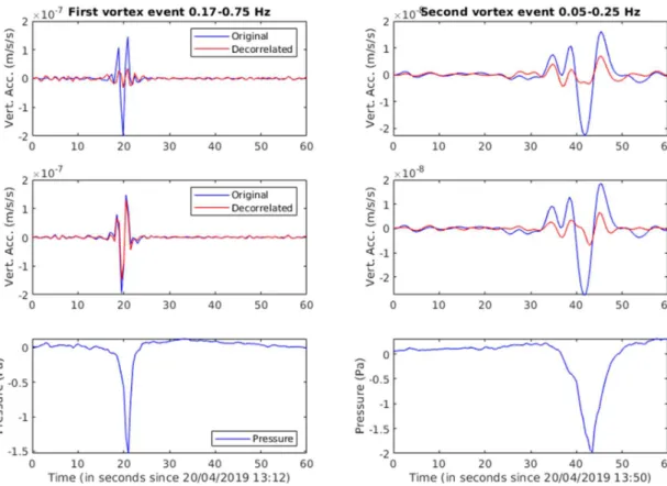
Figure 8 provides a comparison of the two decorrelation methods in the time domain for two pressure drops (convective vortex events) occurring on 20 April 2019 during the Mars day time active period. The method relying on convective vortex modeling provides better performances at high frequencies than the adaptive LMS method, probably because the LMS filter is impacted by the strong wind-generated noise on the vertical component above 0.3 Hz. Similar results are obtained for the two methods at lower frequencies.
4.2. Expected Improvement of Seismic Signal Detection and Analysis
With the current performances of the pressure noise decorrelation methods presented here, we will improve at best the SEIS signal-to-noise ratio by a factor of 2 during the day time period. We do not expect this improved signal-to-noise ratio to significantly increase the detection capabilities of seismic events during the day time. However, one can imagine that the seismic event waveforms could be improved by partly removing the pressure noise, if this noise is contaminating the seismic signal. This application is, however, limited in the framework of seismic events detected up to now, because they occur mainly during periods of low pressure variations, and they have very low amplitudes (Giardini et al., 2020). Their amplitudes are so low that the pressure variations able to induce such signals on the SEIS sensors have an amplitude below the noise level of the APSS pressure sensor. For example, the suspected seismic event recorded on sol 133 has a peak spectral amplitude in velocity smaller than 2×10⁻¹⁰m∕s∕√Hz around 0.5 Hz (Giardini et al., 2020). By
using the ground compliance estimates provided in the next section (≈ 4 × 10⁻⁸m/s/Pa for all components
at 0.5 Hz), this would imply that a pressure signal of peak spectral amplitude 5 × 10⁻³Pa∕√Hz would be
able to generate such a SEIS signal. However, such a pressure signal level is at the noise level of pressure sensor (Figure 1b). Thus, for such small SEIS amplitudes, the pressure noise cannot be decorrelated, and the pressure sensor cannot help to determine if the SEIS signals could be generated by pressure variations.
4.3. Ground Compliance Estimates
As a side product of the pressure noise removal methods, the compliance appears naturally as the response of the adaptive LMS filter and from the coefficients used to remove the convective vortex from the vertical component. Figure 9 presents the compliance estimates obtained by the two methods. The estimates from the adaptive LMS method have been obtained by selecting only the time windows with an average correla-tion with pressure signal larger than 0.5, in order to ensure a proper estimate of the filter relating ground velocities and pressure. The compliance estimates are provided only in frequency ranges for which a signifi-cant coherence is observed between the SEIS components and the pressure. The compliance estimates from the convective vortex events are also presented in Figure 9 in the form of a probability density.
Figure 7. Plots of ground velocity records (in m/s) before and after the decorrelation of the VEL (a, b, d) and POS (c) channels. For each panel, original (blue)
and decorrelated records (red), from top to bottom, vertical, EW, and NS components of SEIS VBB (in m/s) and pressure (in Pa). Ground velocity and pressure records are high pass filtered above 0.01 Hz for VEL channels and above 0.001 Hz for POS channels. Time is expressed in hours LMST, starting at the beginning of sol 169.
The overall values and frequency dependence provided by the two methods are in agreement with simple theoretical predictions for an homogeneous model shown in Figure 9. For the adaptive LMS method, the hor-izontal compliance values obtained along the EW component are larger than along the NS component. This feature may be explained by the local subsurface variations induced by the hollow crater in which INSIGHT landed (about 3 m distance to the Western rim of a 27 m diameter crater, Golombek et al., 2020; Warner et al., 2019). The material inside the crater being softer than outside it, compliance values are expected to be larger in the Eastern direction than along North-South direction. This interpretation is also suggested by analysis of ground response to convective vortices. Due to lower noise and higher sensitivity along the EW component than along the NS component, the EW component provides more reliable compliance estimates. A slope break at 0.1 Hz for the horizontal compliance, and an increase of the compliance with frequency for the vertical compliance, suggests that the subsurface model is heterogeneous. For the method relying on modeling of convective vortices, the slope of the vertical compliance estimates as a function of frequency is larger than for the adaptive LMS method. This suggests a stronger stratification of mechanical properties below SEIS and possible contamination of LMS estimates by other noise sources.
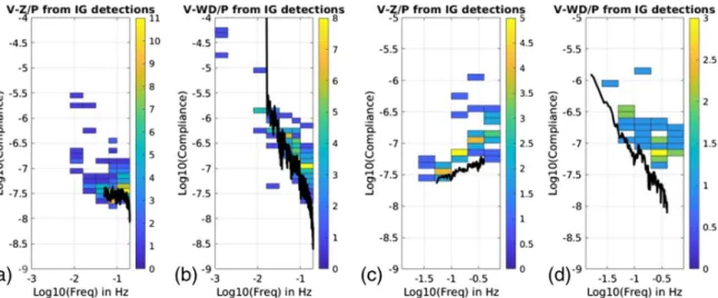
In addition to the compliance estimates flowing down from the decorrelation methods, an automated detection of compliance events has been implemented. To do so, we use band-pass filtered records (in the [
𝑓1, 𝑓2]Hz range) of pressure (P), vertical velocity (Vz), and horizontal velocity along the wind direction (Vh)
to implement a compliance marker defined by IG(t) =
STA(P2)
Journal of Geophysical Research: Planets
10.1029/2019JE006278Figure 8. Comparison of the results of the two decorrelation methods for two convective vortex events occurring on 20 April 2019, respectively, at 13:12 UTC
(on the left) and 13:50 UTC (on the right). From top to bottom decorrelation results for convective vortex modeling (top) and for LMS decorrelation (middle), and the pressure signal (bottom). SEIS vertical component accelerations (in m/s/s) before (blue) and after (red) decorrelation are presented after filtering in the 0.17–0.75 Hz range (resp. 0.05–0.25 Hz) for the first (resp. second) event.
where Hil(Vz) is the Hilbert transform of vertical velocity record, the STA() and LTA() functions stand,
respectively, for Short Term Average performed on the time interval[t − T∕2, t + T∕2]and Long Term Aver-age performed on[t − 20T∕2, t + 20T∕2], and the CCT(X, Y) function stands for Correlation Coefficient between X and Y for the time range[t − T∕2, t + T∕2]. T is defined by T = 3
𝑓1. The last three terms of the
equation should be equal to one if in the time range[t − T∕2, t + T∕2]P, Hil(Vz)and Vhare perfectly
corre-lated, as expected from compliance relation. The first term is an amplitude ratio ensuring that the pressure variations are above the background noise. Then a threshold value is set (typically 0.4) above which the event is considered and the vertical and horizontal compliances are estimated. Finally, in order to ensure that the signal is also above noise on SEIS components, only events withSTA(|VZ|)
LTA(|VZ|) >2are selected. Figure 10 provides
the compliance estimated by this method in the same sol range (169–174) used by the LMS method. A detailed analysis of these compliance estimates is presented in Kenda et al. (2020).
4.4. Limitations
The efficiency of pressure-induced noise removal is currently limited to time periods and SEIS components for which a significant coherence with pressure variations is observed. As shown in Figure 3, despite the fact that large pressure effects are generating the largest signals observed on SEIS, the background noise outside pressure events is dominated by wind noise (Lognonné et al., 2020). This is limiting the efficiency of the pressure decorrelation. Even for signals generated by convective vortices, in order to be able to correct all SEIS components, the characteristics of the vortex and their trajectories must be estimated. In addition, the wind direction information must be taken into account in all methods in order to properly remove the pressure effects on the horizontal components. Finally, as shown by Lognonné et al. (2020), some correla-tions are observed between pressure and wind in different frequency ranges depending on the local time. These correlations may impact compliance estimates because these estimates may contain wind effects in addition to the ground elastic response.
Figure 9. Estimates of V-Z/P vertical compliance (a) and V-H/P horizontal compliance (b) from the spectral shape of LMS FIR filter and of V-Z/P vertical
compliance (c) from convective vortex events using VBB-VEL channels. In panels (a) and (b), the logarithmic average of filter gain is presented for vertical, EW, and NS components, respectively, by red, black, and blue curves. Theoretical predictions with an homogeneous subsurface model are presented assuming only inertial effect on the vertical component (thick dashed blue line) and only tilt effects on the horizontal components (thick dashed red line). On the right panel (c), the color bar indicates the number of convective vortex events providing a given value of vertical compliance.
A general observation is that the wind noise dominates the overall signal recorded by SEIS outside of pres-sure events. If future studies allow this noise source to be removed using TWINS sensors meapres-surements, this will significantly improve the pressure noise removal process.
5. Constraints on Atmospheric Gravity Waves From Seismological Data
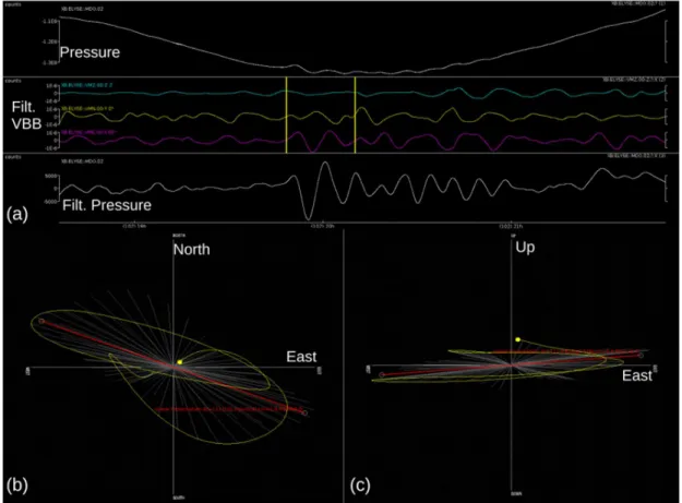
As shown in Figure 2, coherent signals are observed at long periods (400–800 s) between the pressure sensor and the VBB EW component. An example of such an observation is shown in Figure 11 for a pressure per-turbation event on 12 April 2019 at 20:00 UTC. These signals are due to atmospheric gravity waves observed mainly during evening hours and sometimes in the early morning (Banfield et al., 2019). These gravity waves generate pressure waves and ground rotations (compliance tilt effect) that are observed on the hor-izontal components of SEIS. This signal complements the usual atmospheric sensors because it provides new information about these waves: their apparent arrival azimuth.
Figure 10. The logarithm of compliance values estimated using the automated compliance event detection method for POS (a and b) and VEL (c and d)
channels as a function of the logarithm of frequency. Each subplot presents V-Z/P vertical compliance (a and c) and V-WD/P wind direction horizontal compliance (b and d). Color bars indicate the number of events for a given compliance range and frequency range. The black line provides the compliance estimates from the LMS adaptive method for the same sol range (169–174) also presented in Figure 9. Note that the vertical and horizontal scales are different for estimates using VBB-POS (a and b) and VBB-VEL (c and d) channels.
Journal of Geophysical Research: Planets
10.1029/2019JE006278Figure 11. Example of pressure and SEIS signals observed during the passage of a gravity wave. On top (a), from the top to bottom panels: raw pressure record
(in counts), raw records of SEIS-POS components (Z = blue, N = yellow, E = purple), and pressure band pass filtered between 1.1 and 5 mHz. Vertical yellow lines indicate the time period used for polarization analysis in panels (b) and (c). Time (in hours) is starting at 2019-04-12T18:35:57 UTC. On the bottom (b): particle motion of ground velocity in the horizontal North-East (b) and vertical Up-East (c) planes. The best fit to the linear polarization (red curve) provides an azimuth of 111◦and a dip of 5◦.
The wave arrival azimuth is constrained from the polarization of the ground horizontal motions which are expected to be aligned along the wave vector. In the example provided, a fit to a linear polarization of the first two periods of the wave is providing an azimuth of 111◦modulo 180◦(Figure 11b). In order to solve the
180◦ambiguity, we use the fact that arrival of first positive pressure signal tilts the ground downward in that
direction thus generating a negative SEIS signal in that direction. In our case (Figure 11a), a positive signal along the EW component is observed and is associated to the minimum pressure signal arriving slightly after. This means that a positive pressure signal would have generated a negative EW component. Thus, the wave is coming from West, and 111◦is the azimuth of the wave vector. This is confirmed by the fact that the
azimuth of the wind incoming direction observed by TWINS sensors is at 270◦azimuth, thus a wind vector
pointing at 90◦azimuth. The gravity wave apparent velocity being the sum of the wind and the intrinsic
gravity wave velocity, this observation suggests that the wave is propagating southward relative to the wind. Thus, SEIS data indicate that this gravity wave is coming from a source located North-West of the InSight lander. However, due to different sensitivities of the EW and NS components to pressure tilt effects, the apparent azimuth must be corrected from these different sensitivities to obtain the arrival azimuth of the atmospheric wave. These corrections require further data analysis and are beyond the scope of this paper.
6. Conclusion
The coherency between the pressure and seismometer channels demonstrates the impact of pressure pertur-bations on the ground displacements at the InSight location. The largest pressure perturpertur-bations, associated to day time convective vortices and night time gravity waves, generate SEIS signals above other noise sources. The phase and amplitude of the SEIS signals can be explained by compliance theory. Decorrelation meth-ods capable of removing these pressure effects have been implemented with an overall reduction of pressure
noise up to a factor of 2 for VEL channels in the 10–400 mHz frequency range and up to a factor of 4 for POS channels in the 1–4 mHz frequency range. The high efficiency of decorrelation at long periods is encourag-ing for the detection of seismic normal modes of Mars. The amplitude of the compliance relation between the SEIS components and pressure signals is estimated as a by-product of the decorrelation methods. These estimates allow the inversion of subsurface mechanical properties (Kenda et al., 2020). Finally, we demon-strate that the SEIS data allow the apparent arrival azimuths of atmospheric gravity waves to be estimated, thus bringing new information to study these atmospheric phenomena. Further detailed investigations are required to investigate potential correlations between atmospheric parameters that have different influ-ences on SEIS instrument and to quantify the effect of the local subsurface heterogeneities on the horizontal compliance values.
Future implementations of pressure noise decorrelation methods should improve the signal-to-noise ratio of recorded seismic events by focusing on low wind and low pressure variations conditions. A systematic analysis of SEIS records during the periods of atmospheric gravity wave activity will be implemented to understand the night time atmospheric dynamics.
References
Banerdt, W. B., Smrekar, S., Banfield, D., Giardini, D., Golombek, M., Johnson, C., et al. (2020). Initial results from the InSight mission on Mars. Nature Geoscience, 13(3), 183–189. https://doi.org/10.1038/s41561-020-0544-y
Banfield, D., Rodriguez-Manfredi, J. A., Russell, C. T., Rowe, K. M., Leneman, D., Lai, H. R., et al. (2019). InSight Auxiliary Payload Sensor Suite (APSS). Space Science Reviews, 215, 4. https://doi.org/10.1007/s11214-018-0570-x
Beauduin, R, Lognonné, P, Montagner, J., Cacho, S, Karczewski, J., & Morand, M (1996). The effects of the atmospheric pressure changes on seismic signals or how to improve the quality of a station. Bulletin of the Seismological Society of America, 86(6), 1760–1769. Crawford, W. C. (2000). Identifying and removing tilt noise from low-frequency (<0.1 Hz) seafloor vertical seismic data. The Bulletin of the
Seismological Society of America, 90, 952–963. https://doi.org/10.1785/0119990121
Crawford, W. C., Webb, S. C., & Hildebrand, J. A. (1991). Seafloor compliance observed by long-period pressure and displacement measurements. Journal of Geophysical Research, 96, 16. https://doi.org/10.1029/91JB01577
Fayon, L., Knapmeyer-Endrun, B., Lognonné, P., Bierwirth, M., Kramer, A., Delage, P., et al. (2018). A numerical model of the SEIS leveling system transfer matrix and resonances: Application to SEIS rotational seismology and dynamic ground interaction. Space Science
Reviews, 214(8), 119. https://doi.org/10.1007/s11214-018-0555-9
Giardini, D., Lognonné, P., Banerdt, W. B., & Others, M. (2020). The seismicity of Mars. Nature Geoscience. https://doi.org/10.1038/ s41561-020-0539-8
Golombek, M. P., Warner, N. H., Grant, J., Hauber, E., Ansan, V., Weitz, C., et al. (2020). Geology of the InSight landing site, Mars. Nature
Geoscience. https://doi.org/10.1038/s41467-020-14679-1
Haykin, S. (1996). Adaptive filter theory (3rd ed.). Upper Saddle River, NJ, USA: Prentice-Hall, Inc.
InSight Mars SEIS Data Service (2019). SEIS raw data, Insight Mission. IPGP, JPL, CNES, ETHZ, ICL, MPS, ISAE-Supaero, LPG, MFSC. https://doi.org/10.18715/SEIS.INSIGHT.XB_2016
Kenda, B., Drilleau, M., Garcia, R. F., Kawamura, T., Murdoch, N., Compaire, N., et al. (2020). Subsurface structure at the InSight landing site from compliance measurements by seismic and meteorological experiments. Journal of Geophysical Research: Planets, e2020JE006387. https://doi.org/10.1029/2020JE006387
Kenda, B., Lognonné, P., Spiga, A., Kawamura, T., Kedar, S., Banerdt, W. B., et al. (2017). Modeling of ground deformation and shallow surface waves generated by Martian dust devils and perspectives for near-surface structure inversion. Space Science Reviews, 211, 501–524. https://doi.org/10.1007/s11214-017-0378-0
Lognonné, P., Banerdt, W. B., Giardini, D., Pike, W. T., Christensen, U., Laudet, P., et al. (2019). SEIS: Insight's seismic experiment for internal structure of Mars. Space Science Reviews, 215, 12. https://doi.org/10.1007/s11214-018-0574-6
Lognonné, P., Beyneix, J. G., Banerdt, W. B., Cacho, S., Karczewski, J. F., & Morand, M. (1996). Ultra broad band seismology on InterMarsNet. Planetary and Space Science, 44(11), 1237,1241–1239,1249.
Lognonné, W. B., Banerdt, P., & Pike, W. T. (2020). Constraints on the shallow elastic and anelastic structure of Mars from InSight seismic data. Nature Geoscience.
Lognonné, P., & Clévédé, E. (2002). 10 - normal modes of the earth and planets. In W. H. K. Lee, H. Kanamori, P. C. Jennings, & C. Kisslinger (Eds.), International handbook of earthquake and engineering seismology, part A (Vol. 81, pp. 125–cp1). International Geophysics: Academic Press.
Lognonné, P., & Mosser, B. (1993). Planetary seismology. Surveys in Geophysics, 14(3), 239–302.
Lorenz, R. D., Kedar, S., Murdoch, N., Lognonné, P., Kawamura, T., Mimoun, D., & Bruce Banerdt, W. (2015). Seismometer detection of dust devil vortices by ground tilt. The Bulletin of the Seismological Society of America, 105, 3015–3023.
Mimoun, D., Murdoch, N., Lognonné, P., Hurst, K., Pike, W. T., Hurley, J., et al. (2017). The noise model of the SEIS seismometer of the InSight mission to Mars. Space Science Reviews, 211, 383–428.
Murdoch, N., Kenda, B., Kawamura, T., Spiga, A., Lognonné, P., Mimoun, D., & Banerdt, W. B. (2017). Estimations of the seismic pressure noise on Mars determined from large eddy simulations and demonstration of pressure decorrelation techniques for the Insight mission.
Space Science Reviews, 211, 457–483.
Murdoch, N., Mimoun, D., Garcia, R. F., Rapin, W., Kawamura, T., Lognonné, P., et al. (2017). Evaluating the wind-induced mechanical noise on the InSight seismometers. Space Science Reviews, 211, 429–455.
Petrosyan, A., Galperin, B., Larsen, S. E., Lewis, S. R., Määttänen, A., Read, P. L., et al. (2011). The Martian atmospheric boundary layer.
Reviews of Geophysics, 49(3), RG3005.
Sorrells, G. G. (1971). A preliminary investigation into the relationship between long-period seismic noise and local fluctuations in the atmospheric pressure field. Geophysical Journal, 26, 71–82.
Spiga, A., Banfield, D., Teanby, N. A., Forget, F., Lucas, A., Kenda, B., et al. (2018). Atmospheric science with InSight. Space Science Reviews,
214, 109.
Acknowledgments
We acknowledge NASA, CNES, their partner agencies and institutions (UKSA, SSO, DLR, JPL, IPGP-CNRS, ETHZ, IC, MPS-MPG), and the flight operations team at JPL, SISMOC, MSDS, IRIS-DMC, and PDS for providing SEED SEIS data (https://doi. org/10.18715/SEIS.INSIGHT.XB_ 2016). The raw to calibrated data sets of InSight are available via the Planetary Data System (PDS). The figures, figure contents, and input SEIS and APSS data used in this study are available at the following DOI link (https://doi. org/10.5281/zenodo.3741451). The French authors acknowledge the French Space Agency CNES and ANR (ANR-14-CE36-0012-02 and ANR-19-CE31-0008-08) for support in the Science analysis. The co-authors acknowledge Clément Perrin and Eric Beucler for their time-consuming work on InSight event requests that were necessary to increase the sampling rate of data recovered from SEIS and APSS sensors. The co-authors also acknowledge Baptiste Pinot for its work on the removal of “glitches” in SEIS data. R. F. Garcia acknowledges Pedro Rocha Cachim for its contribution to the adaptive LMS decorrelation software during its ISAE-SUPAERO master research training period (2017). French teams acknowledge support from CNES research projects. This study is InSight contribution number 126.
Journal of Geophysical Research: Planets
10.1029/2019JE006278Tanimoto, T., & Wang, J. (2019). Theory for deriving shallow elasticity structure from colocated seismic and pressure data. Journal of
Geophysical Research: Solid Earth, 124, 5811–5835. https://doi.org/10.1029/2018JB017132
Warner, N. H., Golombek, M. P., Grant, J., Wilson, S., Hauber, E., Ansan, V., et al. (2019). Geomorphology and origin of Homestead hollow, the landing location of the InSight lander on Mars. In Lunar and planetary science conference, Lunar and Planetary Science Conference, pp. 1184.
Zürn, W., Exß, J., Steffen, H., Kroner, C., Jahr, T., & Westerhaus, M. (2007). On reduction of long-period horizontal seismic noise using local barometric pressure. Geophysical Journal International, 171, 780–796.
Zürn, W., & Widmer, R. (1995). On noise reduction in vertical seismic records below 2 mHz using local barometric pressure. Geophysical