Any correspondence concerning this service should be sent
to the repository administrator:
[email protected]
This is an author’s version published in:
http://oatao.univ-toulouse.fr/27235
To cite this version: Ochoa Robles, Jesus and Giraud Billoud,
Marialis and Azzaro-Pantel, Catherine and Aguilar-Lasserre,
Alberto Alfonso Optimal Design of a Sustainable Hydrogen
Supply Chain Network: Application in an Airport Ecosystem.
(2019) ACS Sustainable Chemistry & Engineering, 7 (21).
17587-17597. ISSN 2168-0485
Official URL
DOI :
https://doi.org/10.1021/acssuschemeng.9b02620
Open Archive Toulouse Archive Ouverte
OATAO is an open access repository that collects the work of Toulouse
researchers and makes it freely available over the web where possible
Optimal Design of a Sustainable Hydrogen Supply Chain Network:
Application in an Airport Ecosystem
Jesus Ochoa Robles,
†Marialis Giraud Billoud,
†Catherine Azzaro-Pantel,
*
,†and Alberto Alfonso Aguilar-Lasserre
‡†
Laboratoire de Génie Chimique, Université de Toulouse, CNRS, Toulouse, France Toulouse INP, ENSIACET, 4 allée Emile Monso, BP 44362, 31432 Toulouse Cedex 4, France
‡Instituto Tecnológico de Orizaba, Oriente 9, Emiliano Zapata, 94320 Orizaba, Veracruz, Mexico
ABSTRACT: Hydrogen and fuel cell technologies are one solution for addressing the challenges that major airports are facing today, such as upward price trends of liquid hydrocarbon fuels, greenhouse gas emission regulations, and stricter noise and air pollutant emission regulations, especially for on-ground pollution. An airport can also be viewed as the center of a hydrogen ecosystem, around which multiple hydrogen users could be clustered, with cost sharing of hydrogen production and storage occurring among users. The main novelty of the present work is the design of a hydrogen infrastructure irrigated by the airport ecosystem that satisfies the airport ecosystem energy needs. For this purpose, the model development is based on a multiobjective optimization framework designed to consider four echelons: energy sources, hydrogen production, transportation, and storage. The multiperiod problem is then solved using the ε-constraint method.
Two objective functions are involved, that is, the total daily cost (TDC) of the network and an environmental indicator based on the global warming potential. The second innovative contribution is to model the demand uncertainty using fuzzy concepts for a hydrogen supply chain design. Because hydrogen demand is one the most significant parameters, the uncertainty of the demand has been considered using a proposed fuzzy linear programming strategy. The solutions are compared with the original crisp model, giving more robustness to the proposed approach. This work has been performed in the framework of the Hyport meta-project and, in particular, within the “H2modeling” project. This paper focuses on a hydrogen airport ecosystem located in
the department of Hautes-Pyrénées (France). However, the developed methodology could be extended to other hydrogen ecosystems for which deployment involves a multiperiod multi-objective formulation under an uncertain demand.
KEYWORDS: hydrogen supply chain, airport ecosystem, MILP, demand under uncertainty, optimization
■
INTRODUCTIONHydrogen that is produced from renewable sources and is used in fuel cells both for mobile and stationary applications constitutes a very promising energy carrier for the energy transition. The strategic roadmaps1−5 that are currently published regarding the potential of hydrogen at the European, national, and regional levels, as well as the analysis of scientific publications in this field, have identified that even if many of the required technologies are already available today, the deploy-ment of hydrogen infrastructures constitutes a challenging task for the development of a “hydrogen” economy that can achieve competitive costs and mass market acceptance. According to these roadmaps, hydrogen demand for road transportation is assumed to be a major parameter and is likely to grow in three phases according to the energy trends of the 2030 scenario:5
• Infrastructure phase I: the demonstration phase, during which a few large-scale first user centers are situated across Europe.
• Infrastructure phase II: the early commercialization phase with 3−6 user centers per country, possibly including a network of transit roads connecting these centers. • Infrastructure phase III: the full commercialization phase,
which encompasses existing user centers as well as newly developed regions and a dense, long-distance road network. Phase III is assumed to develop in three sub-phases (see ref5for more details).
These large-scale deployment initiatives must be supported by long-term policy frameworks in countries that are early adopters, and they should use current activities as platforms to deploy them at the national scale.6
In that context, a Hydrogen Territory initiative was launched in France in 2016, which aims to demonstrate, on the scale of a particular territory, the techno-economic feasibility and the
environmental benefits of deploying hydrogen in energy networks or local energy applications. The meta-project Hyport proposed by Occitania Region was one of the selected projects: it combines advanced innovation in hydrogen fuel cell applications for aeronautics, green hydrogen production, and H2mobility deployment for the Toulouse international airport,
the Tarbes-Lourdes-Pyrénées regional airport, and the vast urban or rural and touristic perimeters connected to them.
Because of its characteristics, the airport infrastructure is an interesting case study. An airport is a source of emissions that affect the climate, including the emissions generated from activities occurring inside and outside of the airport perimeter fence associated with the operation and use of an airport. The airport infrastructure accounts for 3.9% of the greenhouse gas (GHG) emissions of airplane transportation and its related activities.7Additionally, urban mobility is directly impacted by airport activities: taxis, car rentals, buses, tramways and subways, particular vehicles, lightweight and heavyweight utility vehicles, etc.
In that context, the hydrogen solution seems particularly interesting for the energy supply of the airport infrastructure and utility vehicles in nonpublic areas (ground support). The airport and surrounding areas are important stationary energy demanding zones, and there is an increasing interest in searching for new energy solutions to improve the environmental impact, as well as autonomy, security, and efficiency.
Several studies for the hydrogen supply chain (HSC) design have already been conducted8−13at a larger scale. The most common methodology to solve the HSC problems involves a mixed integer linear programming (MILP) approach.
For example, an HSC for vehicle use was designed in ref13. The design task is formulated as a bicriterion MILP problem. A case study in Great Britain was introduced to illustrate the capabilities of the proposed approach. The model optimizes the economic and environmental objectives. The economic objective is then given by the total discounted cost, and the environmental impact is expressed as the contribution to climate change. Then, the problem is decomposed into two levels. The upper level refers to the so-called master problem, with binary variables related to the selection of different technologies, and the lower level is represented by the original MILP model. The advantage of this methodology is the reduction in the combinatorial complexity of the problem, and thus, its computational effort.
An HSC design for vehicle use is presented in ref 8. The objective is to determine the optimal design of the production− distribution network. The model, based on an MILP formulation with uncertainty modeling introduced into the operating costs of the network, has been applied to a case study in Spain.
A previous work9was devoted to the development of a generic framework that takes the design of an HSC for fuel use into account in the time horizon of 2020−2050 considering the national (France) and regional (Midi-Pyrénées) scales, using many energy sources and embedding the various production and storage technologies, while additionally considering the trans-portation modes to link the hydrogen demand to its supply. A multi-objective formulation is addressed, in which the cost, environmental impact, and safety must be simultaneously considered at an earlier design stage. Even if the methodology was proven to be robust enough to tackle different geographic scales, how the deployment can be operated from typical clusters and industrial ecosystems has not been studied so far.
To fill in this gap, this study is focused on the introduction of the hydrogen solution in an airport ecosystem and its integration into a territory, that is, the “department of Hautes-Pyrénées” in France. This airport is of major importance for the regional economy through its connection with tourism and industrial (aeronautics) activities.
In this work, a regional airport is viewed as the center of a hydrogen ecosystem and the objective is to design a hydrogen infrastructure that is irrigated by the airport ecosystem and satisfies the airport ecosystem energy needs. The approach that will be developed must be generic enough to be applied to other air(port) systems. For this purpose, the methodological framework developed in ref 9 has been used and some constraints have been adapted.
■
HYDROGEN IN AVIATION AND AIRPORT ECOSYSTEM: A REVIEWThe aviation sector is increasingly facing challenges related to the upward price trends of liquid hydrocarbon fuels, GHG emission regulations, and stricter noise and air pollutant emission regulations, especially for on-ground pollution at large airports. Biofuels cannot tackle all these issues, and shifting to hydrogen appears to be a promising alternative, as highlighted in ref14. The replacement of fossil fuels in the aviation industry has been widely studied. The most commonly used fuel for commercial aviation is kerosene, which is a strong pollutant. Therefore, hydrogen and other fuels, such as methane and methanol, have been studied to replace it. In the study reported in ref15, a comparison between kerosene and hydrogen was presented based on their performances and environmental impacts. Hydrogen use in the aviation sector may concern an alternative fuel for future low-emission aircraft. Hydrogen-fueled engines generate no CO2emissions at any point of use, may
reduce NOXemissions, and greatly diminish the emissions of
particulate matter. In ref 16, the GHG emissions of a conventional jet-operated aircraft and one operated by cryogenic liquid H2 over the long term were evaluated. The
author analyzed different introduction rates and emphasized that an efficient, reliable and safe supply chain is a prerequisite for hydrogen deployment. According to these studies, the industry needs to overcome significant technical challenges in designing a hydrogen-powered aircraft for commercial aviation and in sustainably producing enough hydrogen, as well as highlight the needs of a hydrogen infrastructure.17
Hydrogen applications in the aviation industry have been analyzed for specific purposes. In ref 14, an airport liquid hydrogen infrastructure for aircraft auxiliary power units was considered. The incorporation of on-site liquefaction units was considered over a long-term horizon, regarding applications and possible synergies, such as hydrogen-fueled ground support equipment, apron vehicles, and airport-bound vehicles.
Hydrogen is already present in airports worldwide, mostly with the incorporation of refueling stations. Typical examples include international airports in Japan, that is, Kansai18 and Narita,19the Munich airport in Germany,20and the Oslo airport in Norway.21A green hydrogen hub (H2BER) has opened at the new Berlin Brandenburg Airport (BER) under construction in Germany, with hydrogen produced onsite via electrolysis using wind and solar energy.22
Air Liquide and Groupe ADP inaugurated the first public hydrogen station installed in an airport zone in France (Paris-Orly airport area) on 7 December 2017 with the support of the FCH JU (Fuel Cells and Hydrogen Joint Undertaking).23This
initiative is promoting the deployment of “Hype”, the world’s first hydrogen-powered taxi fleet.
In this paper, the uses of hydrogen required in an airport as well as those for the electromobility application of the surrounding Hautes-Pyrénées are considered.
■
MODELING FRAMEWORKFor HSC deployment in Hautes-Pyrénées, the core method-ology developed in ref24was adapted according to the new
characteristics of the system. Let us recall that the model was designed in a generic way to be adapted to different scenarios, for
example, the addition of new energy sources or a new geographic breakdown.
In the initial and generic formulation of the methodology (see
Figure 1), hydrogen can be delivered in a specific physical form i, such as in a liquid or/and gaseous form, produced in a plant type with different production technologies p (i.e., steam methane reforming (SMR), biomass gasification, and electrolysis), distributed by a specific type of transportation modes l and going from location g to g′, referred to as grid squares (g′ is different than g). The HSC is assumed to be demand driven.
The input block corresponds to all the databases, assumptions, and scenarios used for an optimization run. The integration of the mathematical model with a multi-objective optimization approach constitutes the core of the approach. The snapshots and the results involving the decision variables and objective functions are the main outputs.
Figure 1.HSC modelproposed approach following the guidelines proposed in ref9.
Figure 2.Definition of the grids.
Table 1. Percentage of Hydrogen Incorporation for Transportation Purposes for the Considered Scenarios (Relative to the Total Number of Vehicles)
period low demand scenario (%) high demand acenario (%)
2020 1 2
2030 7.5 15
2040 17.5 35
2050 25 50
Table 2. Low-Demand Scenario Values for Each Grid demand of hydrogen per period
(kg/day)
grid 2020 2030 2040 2050 1 North 134 1012 2404 3555
2 East 115 870 2068 3058
3 Centre 149 1126 2675 3955 4 Tarbes (and surroundings) 109 824 1959 2896 5 Lourdes (and surroundings) 103 782 1859 2748 6 Tarbes-Lourdes-Pyrénées airport 288 355 440 538 Table 3. High-Demand Scenario Values for Each Grid
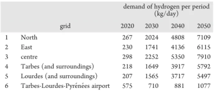
demand of hydrogen per period (kg/day)
grid 2020 2030 2040 2050 1 North 267 2024 4808 7109 2 East 230 1741 4136 6115 3 centre 298 2252 5350 7910 4 Tarbes (and surroundings) 218 1649 3917 5792 5 Lourdes (and surroundings) 207 1565 3717 5497 6 Tarbes-Lourdes-Pyrénées airport 575 710 881 1077
Several data are necessary to design the HSC, including the capital and operational costs (CAPEX and OPEX) for a given facility that will be used for extrapolation purpose, the throughput associated with a given technology, the quantities of the input and output products associated with unit operations of the transformation types, and so forth. Because hydrogen demand is one of the most significant parameters, the uncertainty of the demand has also been taken into account and modeled using the fuzzy linear programming (FLP) strategy proposed by refs 25 and 26, giving more robustness to the proposed approach. The original model involves a multi-objective optimization designed to consider five stages: energy sources, production, transportation, storage, and fueling stations. It was designed to include regional and national levels in order to study the operability and evolution of the system at different scales.
The multiperiod formulation is solved here using the ε-constraint method considering two objective functions to be optimized, that is, the total daily cost (TDC) of the network and the global warming potential (GWP). The instance of the model involved has 3493 continuous variables and 1848 integer variables. The territory has been discretized into 6 grids. Because of these features, a MILP approach is used to model the airport ecosystem HSC. Finally, for the obtained Pareto front, the TOPSIS (technique for order of preference by similarity to ideal solution) methodology is applied to select one of the optimal solutions.
HSC Model Adaptation. As mentioned above, the multiperiod model uses a deterministic MILP approach embedded in a GAMS/CPLEX environment with a multi-objective formulation implemented via the ε-constraint method to generate the Pareto front.
The following notations were used in different constraints: • g and g′: grid squares with g′ ≠ g
• i: product physical form (liquid hydrogen or LH2)
• l: type of transportation modes (tanker truck)
• p: plant type with different production technologies
(SMR, Electrolysis, DisElectrolysis)
• s: storage facility type with different storage technologies
(LH2stock)
In the model, hydrogen can be produced by electrolysis: (1) at or near the site of use in distributed production (DisElectrolysis) or (2) at large facilities and then delivered to the point of use in central production (Electrolysis).
The following hypotheses were made:
• There are no production plants or storage units installed in the department before the first period of simulation. • The learning rate of the system is fixed and equal to 12%
per period.
The risk is not analyzed in this study case, and the optimization objectives retained are the TDC of the network and the total GWP.
Objective Functions.The considered economic objective function is the TDC of hydrogen (TDC, expressed in $ per day) calculated by the addition of capital and operational costs.
TDC FCC TCC CCF FOC TOC γ = + · + + L N MMMM \^]]]] (1)
In this expression, FCC is the facility capital cost ($), TCC is the transportation capital cost ($), and γ is the network operating period (days/year), which is affected by the capital
charge factor (in years). The facility operating cost FOC ($/day) and the transportation operation cost TOC ($/day) are added to the equation to consider the totality of the related costs of the network.
The GWP (GWPtotal, in g eq CO2per day) is given by the
cumulation of GHG emissions related to the total daily production, total daily storage, and total daily transport
GWPtotal=PGWP+SGWP+TGWP (2)
which is the sum of the GWP due to the production facilities type p (PGWP), the storage technology (SGWP), and the daily transport (TGWP).
Uncertainty Modeling. Fuzzy-Constraint Problems.The review proposed by ref27has reported that many works have been devoted to FLP and solution methods. These are typically divided into four areas: (FLP1) linear programming (LP) problems with fuzzy inequalities and crisp objective functions, (FLP2) LP problems with crisp inequalities and fuzzy objective functions, (FLP3) LP problems with fuzzy inequalities and fuzzy objective functions, and (FLP4) LP problems with fuzzy parameters. In the HSC design problem that has been mathematically formulated,9 hydrogen demand has been identified as an uncertain parameter and the HSC design problem refers to the simplest form of FLP, that is, FLP1.
The decision maker can accept a violation of the constraints up to a certain degree, as previously established. This can be formalized for each constraint as ref26
a xi ≤f bi, i=1, . . . , m
This can be modeled using a membership function
x f x x b b x b t x b t : 0, 1 , ( ) 1 ( ) 0 if if if i i i i i i i i i μ → [ ] μ = ≤ ≤ ≤ + ≥ + O P RRRRR Q RRRRR 5
where fiare continuous, nonincreasing functions. The tolerance
that the decision maker is willing to accept up to a value of bi+ ti
is given by the membership function μi. For everyx ∈ 5, μi(x)
represents the degree of fulfillment of the ith constraint. Then, the problem can be solved
z cx
max =
subject to
Ax≤f b x≥0
The approach proposed by ref25through the representation theorem has proven that the problem can be solved via the following parametric LP problem
z cx max = subject to Ax≤g( )α x≥0, α∈ [0, 1] whereg( )α =( ( ), . . . ,g1α gm( ))α ∈ 5m, with gi= fi −1.
To simplify the problem, if all fiare linear
z cx
max =
subject to
x≥0, α∈ [0, 1]
witht=( , . . . ,t1 tm)∈ 5m.
It has been proven28that, when fiis linear, a solution for the
fuzzy constraint problem can be found as if it is a model with nonlinear functions, without any generality loss when assuming linear functions for the fuzzy constraints. Some sample values can be applied to α in the interval [0, 1], and then the model can be solved for every sample value. For example, a step size of 0.25 for sampling α can be transformed into five α-cuts for α = {0; 0.25; 0.5; 0.75; 1}.
Application to Demand Uncertainty Modeling in the HSC Network Design.Hydrogen demand is the only parameter that will be considered as uncertain. In this paper, only the modifications implemented in the HSC model are presented.
The uncertainty has been considered using the following information
• The lower and upper levels of demand have been taken from the analysis conducted in ref15;
• From these values, the average demand is calculated; • The difference between the average and the low/high
demand is calculated, representing an accepted tolerance; • The variable α is then introduced. This variable can take values from 1 to 0 and represents the rate of use of tolerance. A value of α equal to 0.5 corresponds to the average demand.
The constraints that will be modified in the initial crisp version of the model are constraints3−6.
Considering the demand as the right side of the constraints, as in Verdegays’ approach,25the fuzzy right side can be expressed mathematically as
DTig = [DTig +PD (1ig −α)] Ù
(3) Equation 3 must be inserted into constraints 4−6, which replace the corresponding ones in the initial model15
i g DLig +DIig=DTig +PD (1ig −α)∀ , (4) Q Q i g PTig ( ) DT PD (1 ) , l g ilgg ilgg g ig ig ,
∑
α − − = + − ∀ ′ ′ ′ (5) i g ST DT PD (1 ) , ig ig ig β = + −α ∀ (6) • DLig: demand for product i in grid g satisfied by local
production (kg per day). • DI
ig: imported demand of product form i to grid g (kg per
day).
• Qilgg′: flow rate of product i by transportation mode l
between g and g′ (kg per day).
• STig: total average inventory of product form i in grid g
(kg).
• β: storage holding period in number of days (days). PDigis the tolerance of DTig, and α is the rate of use of tolerance.
Six values of the α-cuts were considered: α = {0.16; 0.33; 0.5, 0.66; 0.83; 1}. For each value of the α-cuts, an evaluation of the model was performed.
Data Identification. Geographical Division. Before optimization, the geographical zone is discretized with an independent demand in each grid. A special grid is considered for the airport.
First, a study on the evolution of the municipal population of the department and on its distribution (division in the so-called French “cantons”) to predict the evolution of hydrogen demand (demand as a function of the predicted vehicles’ number) was performed. In the Hautes-Pyrénées, some cantons have a marked urban character: 56% of the inhabitants of the department reside in a cluster (agglomeration of more than 1500 jobs), which is comparable to the regional average (58%). To simplify the problem and homogenize the identified needs, the grids have been grouped according to a geographical distribution, leading to 6 grids.Figure 2represents the selected division.
Hydrogen Needs and Possible Uses.The region considered is the department of Hautes-Pyrénées in France, which was divided into 6 grids with each one of them characterized by a specific demand. The grid division was made following a population density distribution based on statistical data from ref
29 and a geographical distribution criterion (based on proximity), assigning an independent grid for the regional airport.
Originally the demand is fixed and can be satisfied either by local production or by importation from other grids. Two base scenarios were considered for a low and high demand case, based on the previous studies of ref30. The percentage of the hydrogen network incorporation for mobility purposes corre-sponding to each scenario and period is presented in detail in
Table 1.
To identify the demand of vehicles for each grid, a study of their evolution over the last 20 years was conducted, and then a weight factor depending on the population density was assigned. Finally, a 30 year prediction following the observed trend was conducted for demand estimation. The categories considered are particular and commercial vehicles, buses, trucks, and lightweight vehicles (≤3.5 t) and agricultural tractors. The hydrogen demand is a function of the average distance covered in km/year and of the standard fuel economy for each category. The specific energy needs of the airport grid have also been studied in more detail. They involve different categories, that is, lighting, heating, generator power units, daily airplane move-ment, and the vehicle fleet. Each one of them was identified with the collaboration of the airport staff. The final aim was to cover 20% of the heating demand and 100% of the demand required by the vehicle fleet, generator, and security power units by 2050. As the facilities are not yet fully deployed, the general demand was increased by 15% for each period, following the airport’s expected development scenario.
The assumptions based on the data provided by the airport are:
• The flight frequency ascends to 14 flights per day. • The 90, 120, and 140 kVA generator units work 3 h per
day.
• The 100, 250, and 650 kVA security system units can provide energy for 48 h if needed.
• The utility vehicles include nine 400 kW towing tractors functioning 4 h per day, two 3 kW forklifts functioning 7 h per day, and five lightweight vehicles with a medium distance of 10 000 km/year (captive fleet).
• The hydrogen consumption was calculated for each period considering the medium distances covered by the buses and the number of planes per day.
The estimation scenarios of the demand forecast for hydrogen in the short, medium, and long term with market penetration are presented inTables 2and3.
Energy Sources.To produce hydrogen, five renewable energy sources could be considered, that is, photovoltaic, wind, hydropower, biogas, and geothermal.
Hydropower is the principal energy source of the department, that is, 950 MWp are installed in 130 hydraulic plants. Only the run-of-river power plants were considered, as the production of impoundment facilities is essentially used as a water reservoir, and the pumped storage systems are used for electricity generation during high-demand peaks.
Even though the solar plants did not have any significant evolution since 2012, three soil installations can be found in the
region. Over the next few years, some projects will probably come to fruition.
Regarding biogas production via methanization, there is one plant installed with a cogeneration capacity of 2500−3000 kW h of electricity per month. There are currently future projects under investigation on a medium-term basis.
Because of the regional characteristics, no wind source has been considered.
Geothermal energy is used only for particular purposes, and even though there is a large potential in the north of the department, the available data are as of now insufficient to make future predictions.
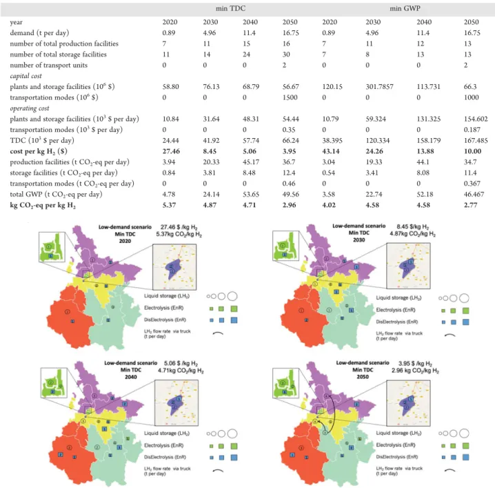
Given the study case constraints, only hydraulic and solar energy resources were finally considered. Additionally, accord-Table 4. Mono-objective Low-Demand Scenario Detailed Optimization Results
min TDC min GWP
year 2020 2030 2040 2050 2020 2030 2040 2050
demand (t per day) 0.89 4.96 11.4 16.75 0.89 4.96 11.4 16.75 number of total production facilities 7 11 15 16 7 11 12 13 number of total storage facilities 11 14 24 30 7 8 13 13
number of transport units 0 0 0 2 0 0 0 2
capital cost
plants and storage facilities (106$) 58.80 76.13 68.79 56.67 120.15 301.7857 113.731 66.3
transportation modes (106$) 0 0 0 1500 0 0 0 1000
operating cost
plants and storage facilities (103$ per day) 10.84 31.64 48.31 54.44 10.79 59.324 131.325 154.602
transportation modes (103$ per day) 0 0 0 0.35 0 0 0 0.187
TDC (103$ per day) 24.44 41.92 57.74 66.24 38.395 120.334 158.179 167.485
cost per kg H2($) 27.46 8.45 5.06 3.95 43.14 24.26 13.88 10.00
production facilities (t CO2-eq per day) 3.94 20.33 45.17 36.7 3.04 19.33 44.1 34.7
storage facilities (t CO2-eq per day) 0.84 3.81 8.48 12.4 0.54 3.41 8.08 11.4
transportation modes (t CO2-eq per day) 0 0 0 0.46 0 0 0 0.367
total GWP (t CO2-eq per day) 4.78 24.14 53.65 49.56 3.58 22.74 52.18 46.467
kg CO2-eq per kg H2 5.37 4.87 4.71 2.96 4.02 4.58 4.58 2.77
ing to ref31, it has been highlighted that there is no cause for concern regarding either the impact of the glint and glare from solar PV or the infringement on airspace or interference with communications equipment within the perimeter of the airport. Numerous airports around the world have already begun to use solar energy to produce power for their needs.
■
RESULTSMono-objective Optimization. Two mono-objective optimizations were performed with the low-demand scenario,
minimizing the GWP and the TDC. The results are presented in
Table 4.
Figures 3 and 4 show the obtained network for both
optimization strategies. In all the maps provided, the number of plants is indicated inside the symbols used for a technology representation.
Figure 3represents the evolution of the supply chain for a period step of 10 years by optimizing the cost of hydrogen. Transportation is not considered due to weak demand in LH2.
The minimal cost in the last period is 3.95 $/kg H2with 2.96 kg
eq CO2/kg H2. The capital investment in 2030 has the highest
value regarding both the production units and storage facilities needed to develop the network and satisfy hydrogen needs. The major production technologies are electrolysis and diselectrol-ysis from both considered sources of renewable energy.
When TDC is minimized (Figure 3), during the first period hydrogen is produced by the distributed electrolysis plants in each region, with an additional electrolyzer in the airport grid. During the other periods, priority is given to the installation of distributed plants, mainly due to the weak demand. The average hydrogen cost is 11.23 $/kg H2. Almost the same distribution
can be found when GWP is minimized (Figure 4). The average CO2 emissions are 3.99 kg CO2 eq per kg H2. The main
difference between the two cases lies in number of electrolyzers installed and the size of the facility plants.
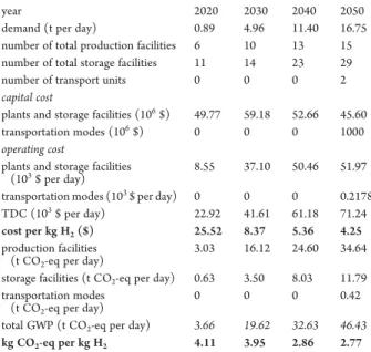
Multi-objective Optimization.The first step is to consider a scenario with low demand. As can be observed inTable 5, the cost decreases drastically from the first period (25.52 $/kg H2)
to the last one (4.25 $/kg H2). This can be explained by the
initial investment required to implement the HSC network and the low demand for the first period. The demand increase along all periods helps to reduce the cost per kg of H2. The same
situation occurs with CO2emissions, reaching 2.77 kg CO2-eq
per kg H2in the last period.
Figure 4.Maps for the low-demand scenario (min GWP).
Table 5. Multi-objective Optimization Results for the HSC
year 2020 2030 2040 2050
demand (t per day) 0.89 4.96 11.40 16.75 number of total production facilities 6 10 13 15 number of total storage facilities 11 14 23 29 number of transport units 0 0 0 2
capital cost
plants and storage facilities (106$) 49.77 59.18 52.66 45.60
transportation modes (106$) 0 0 0 1000
operating cost
plants and storage facilities
(103$ per day) 8.55 37.10 50.46 51.97
transportation modes (103$ per day) 0 0 0 0.2178
TDC (103$ per day) 22.92 41.61 61.18 71.24
cost per kg H2($) 25.52 8.37 5.36 4.25
production facilities (t CO2-eq per day)
3.03 16.12 24.60 34.64 storage facilities (t CO2-eq per day) 0.63 3.50 8.03 11.79
transportation modes (t CO2-eq per day)
0 0 0 0.42
total GWP (t CO2-eq per day) 3.66 19.62 32.63 46.43
Figure 5 shows the evolution of the supply chain for the periods from 2020 until 2050, considering the low-demand scenario. In the first period, there are only distributed plants due to low hydrogen. The cost of the network for this period is 25.52 $/kg H2with 4.08 kg CO2eq kg H2. The investment costs of the
supply chain are high in the first period because there is no production plant or previously installed storage facility. With the development of the network, the costs reduce until reaching 4.25 $/kg H2in 2050. Between the second and the third periods the
demand increases, giving the possibility to incorporate transport units between grids, and consequently strongly lowering the hydrogen cost. As the model allows the elimination of plants from one period to another, the distributed network moves
toward a centralized design, with production plants near the renewable energy sources and hydrogen transportation to the other grids. For the airport grid, the demand is low enough to be satisfied by local production so that no changes occur from one period to another.
Regarding CO2emissions, there is a reduction between the
five periods reaching 2.77 kg CO
2-eq per kg H2. These results
depend strongly on a study case for which the energy resources are 100% renewable and mostly from hydraulic power plants, which exhibit the lowest GWP values.
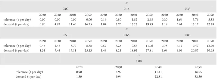
Uncertain-Demand Scenario.For this case, the demand is not fixed and may vary between the values of the low demand and the high demand. The tolerance is the difference between
Figure 5.Maps for low-scenario demand in the multi-objective formulation (min TDC and min GWP).
Table 6. Values of the Demand According to the α-Cut
α
0.00 0.16 0.33
2020 2030 2040 2050 2020 2030 2040 2050 2020 2030 2040 2050 tolerance (t per day) 0.00 0.00 0.00 0.00 0.14 0.80 1.82 2.68 0.30 1.64 3.76 5.53 demand (t per day) 0.90 4.97 11.40 16.75 1.04 5.76 13.23 19.43 1.19 6.61 15.17 22.28
α
0.50 0.66 0.83
2020 2030 2040 2050 2020 2030 2040 2050 2020 2030 2040 2050 tolerance (t per day) 0.45 2.48 5.70 8.38 0.59 3.28 7.53 11.06 0.75 4.12 9.47 13.90 demand (t per day) 1.35 7.45 17.11 25.13 1.49 8.25 18.93 27.81 1.64 9.09 20.87 30.65
α 1.00
2020 2030 2040 2050
tolerance (t per day) 0.90 4.97 11.41 16.75
the high and low demand, and the concept of α is introduced as the percentage of tolerance that will be added to the low demand.25,27Table 6shows the demand used for each α-value. For each α-value, a bicriteria optimization procedure has been implemented, leading to the set of solutions constituting the Pareto front, from which the M-TOPSIS procedure is then applied. The criteria (average values over the periods) relative to the compromise solution of the HSC network finally obtained are presented inTable 7, and the instances obtained when α is
equal to 0; 0.16; 0.33; and 0.50 are shown inTable 8, where the relative deviation when α is equal to 0 is presented.
As expected, the unitary cost of hydrogen decreases when α increases, that is, with the first α-value of 0.16, the average cost is of 5.28 $/kg H2. As the α-value increases, the unitary cost
decreases, leading to 4.53 $/kg H2with α equal to 1.
The detailed results are presented inTable 8.
A robustness study can also be conducted from the optimization results. Let us consider the HSC network configuration obtained when α is equal to 0.33. The network, Table 7. Results of the HSC Network Solutions for the Different α-Cuts (Average Values over the Four Periods)
αvalue
0.16 0.33 0.50 0.66 0.83 1.00
TDC (M$ per day) 208.46 231.6 254.06 276.6 287.01 308.47 relative deviation (reference α = 0) 6% 17.59% 29.00% 40.44% 45.73% 56.62% unit cost ($ per kg H2) 5.28 5.12 4.98 4.87 4.6 4.53
relative deviation (reference α = 0) 9% 11.61% 14.03% 15.93% 20.59% 21.80% GWP (t CO2-eq per day) 154.09 181.47 204.92 229.95 262.58 299.04
relative deviation (reference α = 0) 51% 77.32% 100.23% 124.69% 156.58% 192.20% GWP (kg CO2-eq per kg H2) 3.9 4.01 4.01 4.05 4.21 4.39
relative deviation (reference α = 0) 30% 33.22% 33.22% 34.55% 39.87% 45.85% αvalue
208.46 231.6 254.06 276.6 287.01 308.47 TDC (M$ per day) 6% 17.59% 29.00% 40.44% 45.73% 56.62% relative deviation (reference α = 0) 5.28 5.12 4.98 4.87 4.6 4.53 unit cost ($ per kg H2) 9% 11.61% 14.03% 15.93% 20.59% 21.80%
relative deviation (reference α = 0) 154.09 181.47 204.92 229.95 262.58 299.04 GWP (t CO2-eq per day) 51% 77.32% 100.23% 124.69% 156.58% 192.20%
relative deviation (reference α = 0) 3.9 4.01 4.01 4.05 4.21 4.39 GWP (kg CO2-eq per kg H2) 30% 33.22% 33.22% 34.55% 39.87% 45.85%
relative deviation (reference α = 0) 208.46 231.6 254.06 276.6 287.01 308.47 Table 8. Optimal HSC Network configurations Obtained for α = 0, α = 0.16, α = 0.33, and α = 0.50
which has been obtained from the successive use of the multi-objective optimization procedure and the MCDM technique, is perfectly consistent with the corresponding demand. However, if the demand does not reach the maximal expected value, this will result in higher values for all criteria. To check if an acceptable range for the criteria values can still be obtained even if the network is over dimensioned for this demand level, a postoptimal analysis is then performed using the given network and the lowest value of the demand (seeTable 9). It can be highlighted that if the demand is not reached, the cost increases while the CO2emissions remain stable. It is then up to the
decision maker to define which degree of cost uncertainty is acceptable at the design stage for HSC deployment.
■
CONCLUSIONS AND PERSPECTIVESAn HSC model based on a multi-optimization framework has been adapted in this work for an airport ecosystem. The viability of the HSC has been analyzed along different periods. In the last period (2050), the cost and the CO2emissions per kg of H2
reach their lowest values, mostly due to the maturity of the HSC. In the first period, the cost is still prohibitive due to HSC deployment (plants and storage units) and the subsequent low demand.
The CO2emissions are very low due to the renewable source
used, in this case mainly hydropower. This type of energy has the lowest pollution and is also the cheapest, resulting in very similar solutions between periods.
The application of the airport system is a very interesting hydrogen platform, as it permits the introduction of hydrogen to a strategic point by not only considering aircraft utilization but also the activities generated by the airport (eco-mobility, tourist interest, etc.).
The conceptual project design described above may be replicated in other regions where there is an (air)port ecosystem. This modeling approach can be useful for considering various ways to cluster multiple hydrogen users around an (air)port ecosystem, with the cost sharing of hydrogen production and storage among users and to develop rollout strategies.
This work thoroughly assessed the role of a hydrogen market segment centered around airport needs. However, the methodological framework is generic enough to be applied to the market opportunities for green hydrogen, that is, industry and mobility scenarios on a larger scale, which represents a key market for achieving sustainable growth. Some perspectives can also be highlighted. For example, other parameters can be modeled under uncertainty, such as the demand, costs, or prices involved in the model. The TDC can be substituted by the use of discounted costs associated with each time slot. The influence of other parameters, such as the safety stock period, new tube
trailer capacities, and the use of pipelines, could also be evaluated in future case studies.
■
AUTHOR INFORMATION Corresponding Author *E-mail:[email protected]. ORCID Catherine Azzaro-Pantel:0000-0001-5832-5199 NotesThe authors declare no competing financial interest.
Some icons have been adapted from images designed by iconicbestiary/Freepik. Designed by macrovector/Freepik (https://www.freepik.com/macrovector).
■
ACKNOWLEDGMENTSThe authors would like to sincerely thank Pascal Le Houelleur, Director of Pyrenia, and Mathilde Convert (AD’OCC), who kindly shared their knowledge or provided data on various aspects of the Tarbes-Lourdes-Pyrénées airport.
■
REFERENCES(1) FCH JU. 2019, Hydrogen Roadmap Europe: A Sustainable Pathway for the European Energy Transition.https://www.fch.europa. eu/news/hydrogen-roadmap-europe-sustainable-pathway-european-energy-transition(accessed July 27, 2019).
(2) ADEME. 2018, Technical Review: The Role of Hydrogen in the
Energy Transition (accessed July 27, 2019).
(3) IEA. 2019, The Future of Hydrogen; IEA: Paris,www.iea.org/ publications/reports/thefutureofhydrogen/(accessed July 27, 2019).
(4) Hydrogen Council. Hydrogen Scaling up. A Sustainable Pathway for the Global Energy Transition. Nov-2017. (Online). Available:
http://hydrogencouncil.com/wp-content/uploads/2017/11/ Hydrogen-scaling-up-Hydrogen-Council.pdf (accessed: 27-July 27, 2019).
(5) Ozkan, N. A Review of Hydrogen Demands in National Roadmaps; Policy Studies Institute, 2009.
(6) Hydrogen Council. Hydrogen Scaling up. A Sustainable Pathway for the Global Energy Transition. Nov-2017. (Online). Available:
http://hydrogencouncil.com/wp-content/uploads/2017/11/ Hydrogen-scaling-up-Hydrogen-Council.pdf(accessed Jan 4, 2018).
(7) MADEELI. Presentation du meta-projet Hyport en vue de la
labellisation“Territoires Hydrogène. Dossier Principal. Sept 30, 2016. (8) Sabio, N.; Gadalla, M.; Guillén-Gosálbez, G.; Jiménez, L. Strategic planning with risk control of hydrogen supply chains for vehicle use under uncertainty in operating costs: a case study of Spain. Int. J.
Hydrog. Energy 2010, 35, 6836−6852.
(9) De León Almaraz, S. Multi-objective optimisation of a hydrogen supply chain. PhD Thesis, Université de Toulouse, 154236012, 2014.
(10) Agnolucci, P.; Akgul, O.; McDowall, W.; Papageorgiou, L. G. The importance of economies of scale, transport costs and demand patterns in optimising hydrogen fuelling infrastructure: An exploration with
Table 9. Robustness Analysis of the Optimal Configurations
α= 0.33 α= 0.66 α= 1.00
2020 2030 2040 2050 2020 2030 2040 2050 2020 2030 2040 2050 TDC (M$ per day) 23.84 45.64 66.43 80.96 25.71 54.01 80.25 95.61 27.42 58.69 87.75 102.61 relative deviation (reference α = 0) 4% 10% 9% 14% 12% 30% 31% 34% 20% 41% 43% 44% unit cost ($ per kg H2) 26.79 9.20 5.83 4.83 28.89 10.89 7.04 5.71 30.81 11.83 7.70 6.13
relative deviation (reference α = 0) 5% 10% 9% 14% 13% 30% 31% 34% 21% 41% 44% 44% GWP (t CO2-eq per day) 3.66 19.71 32.78 46.51 3.68 19.68 32.71 46.43 3.67 19.75 32.75 46.65
relative deviation (reference α = 0) 0% 0% 0% 0% 1% 0% 0% 0% 0% 1% 0% 0% kg CO2-eq per kg H2 4.11 3.97 2.88 2.78 4.13 3.97 2.87 2.77 4.12 3.98 2.87 2.79
SHIPMod (Spatial hydrogen infrastructure planning model). Int. J.
Hydrog. Energy 2013, 38, 11189−11201.
(11) Almansoori, A.; Shah, N. Design and operation of a future hydrogen supply chain: Multi-period model. Int. J. Hydrog. Energy 2009,
34, 7883−7897.
(12) Almansoori, A.; Shah, N. Design and operation of a stochastic hydrogen supply chain network under demand uncertainty. Int. J.
Hydrog. Energy 2012, 37, 3965−3977.
(13) Guillén-Gosálbez, G.; Mele, F. D.; Grossmann, I. E. A bi-criterion optimization approach for the design and planning of hydrogen supply chains for vehicle use. AIChE J. 2010, 56, 650−667.
(14) Stiller, C.; Schmidt, C. Airport Liquid Hydrogen Infrastructure for
Aircraft Auxiliary Power Units, presented at the 18th World Hydrogen
Energy Conference 2010 - WHEC 2010: Essen, 2010; Vol. Parallel Sessions Book 5: Strategic Analyses/Safety Issues/Existing and Emerging Markets.
(15) Yılmaz, İ.; İlbaş, M.; Taştan, M.; Tarhan, C. Investigation of hydrogen usage in aviation industry. Energy Convers. Manag. 2012, 63, 63−69.
(16) Janić, M. Greening commercial air transportation by using liquid hydrogen (LH2) as a fuel. Int. J. Hydrog. Energy 2014, 39, 16426− 16441.
(17) Lee, J.; Mo, J. Analysis of Technological Innovation and Environmental Performance Improvement in Aviation Sector. Int. J.
Environ. Res. Public. Health 2011, 8, 3777−3795.
(18) Iwatani Europe: Hydrogen Station. (Online). Available:http:// www.iwatani-europe.de/hydrogen-station.html (accessed July 20, 2017).
(19) Hydrogen - Renewable Energy - Idemitsu Kosan Global. (Online). Available: http://www.idemitsu.com/products/energy/ battery/index.html(accessed July 20, 2017).
(20) Munich Airport - Zone 3 - Cargo. (Online). Available:https:// www.munich-airport.de/en/micro/technik/zonen/fracht1/index.jsp
(accessed July 20, 2017).
(21) Prime Minister opens hydrogen filling station at Oslo Airport. (22) Green hydrogen facility opens at Berlin airport, Fuel Cells Bull.., vol. 2014, no. 5, p. 1, May . doi.org/DOI: 10.1016/S1464-2859(14) 70122-1.
(23) Fuel Cells and Hydrogen. Fuel Cells and Hydrogen. Joint Undertaking. (Online). Available: http://www.fch.europa.eu/ (ac-cessed May 8, 2018).
(24) Ochoa Robles, J.; De-León Almaraz, S.; Azzaro-Pantel, C. Optimization of a Hydrogen Supply Chain Network Design by Multi-Objective Genetic Algorithms. In Computer Aided Chemical Engineering; Kravanja, Z., Bogataj, M., Eds.; Elsevier, 2016; vol. 38, pp 805−810.
(25) Verdegay, J. L. Fuzzy mathematical programming. In Fuzzy
Information and Decision Processes; Gupta, M. M., Sanchez, E., Eds.;
Springer: North-Holland, Amsterdam, 1982; pp 231−237.
(26) Villacorta, P. J.; Rabelo, C. A.; Pelta, D. A.; Verdegay, J. L. FuzzyLP: An R Package for Solving Fuzzy Linear Programming Problems. Granular, Soft and Fuzzy Approaches for Intelligent Systems; Springer: Cham, 2017; pp 209−230.
(27) Ebrahimnejad, A.; Verdegay, J. L. A Survey on Models and Methods for Solving Fuzzy Linear Programming Problems. Fuzzy Logic
in Its 50th Year; Springer: Cham, 2016, pp 327−368.
(28) Delgado, M.; Herrera, F.; Verdegay, J. L.; Vila, M. A. Post-optimality analysis on the membership functions of a fuzzy linear programming problem. Fuzzy Sets Syst. 1993, 53, 289−297.
(29) Insee - Institut National de la Statistique et des Études Économiques. [Online]. Available: https://www.insee.fr/fr/accueil
[accessed Jun 15, 2017].
(30) Salingue, C. Optimisation de la Chaîne Logistique de L’hydrogène en
Région Midi-Pyrénées; ENSEEIHT and ENSIACET (INP): Toulouse,
France, Memoire de stage, Sept 2012.
(31) Solar Trade association. Impact of Solar PV on Aviation and Airports, 2016. http://www.solar-trade.org.uk/wp-content/uploads/ 2016/04/STA-glint-and-glare-briefing-April-2016-v3.pdf [accessed July 27, 2019].