Optimization of a hydrogen supply chain network design under demand uncertainty by multi-objective genetic algorithms

(1)

HAL Id: hal-03125630

https://hal.archives-ouvertes.fr/hal-03125630

Submitted on 29 Jan 2021

HAL is a multi-disciplinary open access

archive for the deposit and dissemination of

sci-entific research documents, whether they are

pub-lished or not. The documents may come from

teaching and research institutions in France or

abroad, or from public or private research centers.

L’archive ouverte pluridisciplinaire HAL, est

destinée au dépôt et à la diffusion de documents

scientifiques de niveau recherche, publiés ou non,

émanant des établissements d’enseignement et de

recherche français ou étrangers, des laboratoires

publics ou privés.

Optimization of a hydrogen supply chain network design

under demand uncertainty by multi-objective genetic

algorithms

Jesús Robles, Catherine Azzaro-Pantel, Alberto Aguilar-Lasserre

To cite this version:

Jesús Robles, Catherine Azzaro-Pantel, Alberto Aguilar-Lasserre. Optimization of a hydrogen supply

chain network design under demand uncertainty by multi-objective genetic algorithms. Computers &

Chemical Engineering, Elsevier, 2020, 140, pp.106853. �10.1016/j.compchemeng.2020.106853�.

�hal-03125630�

(2)

Any correspondence concerning this service should be sent

to the repository administrator:

[email protected]

This is an author’s version published in:

http://oatao.univ-toulouse.fr/27269

To cite this version: Robles, Jesús

and Azzaro-Pantel,

Catherine

and Aguilar-Lasserre, Alberto Optimization of a hydrogen

supply chain network design under demand uncertainty by

multi-objective genetic algorithms. (2020) Computers & Chemical

Engineering, 140. 106853. ISSN 0098-1354

Official URL

DOI :

https://doi.org/10.1016/j.compchemeng.2020.106853

Open Archive Toulouse Archive Ouverte

OATAO is an open access repository that collects the work of Toulouse

researchers and makes it freely available over the web where possible

(3)

Optimization

of

a

hydrogen

supply

chain

network

design

under

demand

uncertainty

by

multi-objective

genetic

algorithms

Jesus

Ochoa

Robles

a

_,

_Catherine

_{Azzaro-Pantel}

a, ∗

,

Alberto

Aguilar-Lasserre

b

a Université de Toulouse, Laboratoire de Génie Chimique, LGC UMR CNRS 5503 INP UPS TOULOUSE INP ENSIACET 4 allée Emile Monso – BP 44362

-31432, Toulouse Cedex 4, France

b Instituto Tecnológico de Orizaba, Oriente 9, Emiliano Zapata, Orizaba 94320, Ver., Mexico

a

b

s

t

r

a

c

t

Hydrogeniscurrentlyconsideredoneofthemostpromisingsustainableenergycarriersformobility applications. A model of the hydrogen supply chain (HSC) based on MILP formulation (mixed integer linear programming)in amulti-objective, multi-period formulation,implemented via the ε -constraint method togenerate the Pareto front, wasconducted in a previous workand applied to the Occitania region of France. Three objective functions have been considered, i.e., the levelized hydrogen cost, the global warming potential, and a safety risk index. However, the size of the problem mainly induced by the number of binary variables often leads to difficulties in problem solution.Thefirstinnovative partofthiswork exploresthepotentialofgeneticalgorithms(GAs)via a variant of the non-dominated sorting genetic algorithm (NSGA-II) to manage multi-objective formulation to produce compromise solutions automatically. The values of the objective functions obtained by the GAs in the mono-objective formulation exhibit the same order of magnitude as those obtained with MILP, and the multi-objective GAyields a Pareto front of better quality with well-distributed compromise solutions. The differences observed between the GA and the MILP approaches can be explained by way of managing the constraints and their different logics. The second innovative contribution is the modelling of demand uncertainty using fuzzy concepts for HSC design.Thesolutions arecomparedwiththeoriginal crispmodelsbasedoneither MILPorGA, giving morerobustnesstotheproposedapproach.

1. Introduction

Hydrogen is one of the most promising energy carriers in the search for a resilient, sustainable energy mix to be used in different applications, such as stationary fuel cell systems and electro- mobility applications.

The challenge of developing a future commercial hydrogen economy involves the deployment of a viable hydrogen supply chain (HSC), considering the most energy-efficient, environmen- tally benign, safe and cost-effective pathways to deliver hydrogen to the consumer ( IEA 2017). The HSC for the mobility market

Acronyms: CCS, Carbon Capture and Storage; GA, Genetic Algorithm; GHG, Greenhouse Gas; GWP, Global Warming Potential; HSC, Hydrogen Supply Chain; MCDM, Multi-Criteria Decision Making; MILP, Mixed Integer Linear Programming; MINLP, Mixed Integer Nonlinear Programming; NSGA-II, Non-dominated Sorting Ge- netic Algorithm; SCND, Supply Chain Network Design; SMR, Steam Methane Re- forming; TDC, Total Daily Cost; TOPSIS, Technique for Order Preference by Similarity to Ideal Solution.

∗ _{Corresponding author.}

E-mail address: [email protected] (C. Azzaro-Pantel).

is defined as a system of activities from suppliers to customers. The activities include the choice of the energy source, production technology, storage, and distribution until reaching refuelling stations. Hydrogen can be produced either centrally (similar to ex- isting gasoline supply chains) or distributed at forecourt refuelling stations as small-scale units that can produce H 2 close to the use

point in small quantities.

The network design of the HSC applied to fuel cell electric vehicles has been studied in various works, as highlighted in Table1. The most common methodology to solving the HSC problems involves a mixed integer linear programming (MILP) approach.

In the same vein, the work conducted in ( De-León Almaraz et al., 2014) solved a multi-period model using a deterministic MILP approach embedded in a GAMS/CPLEX environment with a multi-objective formulation implemented via the

ε

-constraint method to generate the Pareto front. The final choice for the HSC was performed through a multiple criteria decision-making process (i.e., technique for order of preference by similarity to ideal solution, TOPSIS). The modelling approach used one economic objective based on hydrogen total daily cost (TDC), one environmental https://doi.org/10.1016/

(4)

Table 1

Territorial approach of the HSC studies. Approach Territorial scale Uncertain

parameters Author(s) Time scale (periods) _Mono _Multi Objective(s) Energy source Observations MILP Great Britain No ( De León Almaraz, 2014 ) X Cost, Ecological,

Safety risk Natural gas, coal, biomass

ε-constraint method for the multi-period problem

( Guillén-Gosálbez et al., 2010 ) 5 (5 years) Cost, Ecological The Pareto front is obtained by the ε-constraint method

( Ren et al., 2007 ) 9 (2020-2060) Financial Coal, Natural gas, Biomass

(CCS), renewable Development of a spatially-explicit MILP model, called SHIPMod (Spatial Hydrogen Infrastructure Mode) ( Kim et al., 2011 ) 4 (seasons) Wind, renewable sources

( Deb et al., 2002 ) x Natural gas, coal, biomass, other renewable sources ( Ebrahimnejad and

Verdegay, 2016 ) 5 (2005-2034)

Demand ( Almansoori and Shah, 2012 ) 3 (2005-2022) Demand uncertainty is modelled using scenario-based-approach Korea ( Kim et al., 2008 ) X Natural gas, renewable

sources Demand uncertainty is modelled using scenario-based-approach Germany No ( Delgado et al., 1993 ) X Natural gas, Coal (CCS),

Biomass Jeju Island,

Korea ( McKinsey&Company, 2010 ) 12 (months) Biomass A sensitivity analysis is conducted to provide insights into the efficient management of the

biomass-to-hydrogen supply chain Midi-Pyrénées,

France ( De-León Almaraz et al., 2014 ) 4 (2010-2050) Cost, Ecological, Safety risk Natural gas, photovoltaic, wind, hydro, nuclear

ε-constraint method for the multi-period problem Regional level ( Bento, 2010 ) 5 (2004-2038) Financial,

Ecological Natural gas, coal, biomass, other renewable sources The territorial scale is not specified, only defined as a "geographical region"

China ( McKinsey and Company 2010 ) 5 (2010-2034)

Malaysia ( Almansoori and Shah, 2006 ) x Cost Natural gas, coal, biomass,

water electrolysis Two methods for demand determination: one based on the prediction of vehicle numbers and the other based on the supply of gasoline and diesel

Korea ( Murthy Konda et al., 2011 ) X Financial, Safety Natural gas, renewable

sources The relative risk index proposed is based on the relative risks of individual components of hydrogen infrastructure

Spain Fuel price ( Sabio et al., 2010 ) 8 Financial, Risk Natural gas, coal (CCS), Biomass, renewable resources

The uncertainty is associated to the operating costs

MINLP-GIS Pakistan No ( Ochoa Robles et al., 2018 ) X Financial Biomass Fuzzy multiple

objective programming

Korea ( Dagdougui et al., 2012 ) X Financial,

Ecological, Risk Natural gas (CCS), other renewable sources Genetic

Algorithms Midi-Pyrénées, France ( Kim and Moon, 2008 ) 4 (2010-2050) Natural gas, renewable sources MINLP Unspecified ( European Commission 2008 ) Financial,

(5)

objective based on GHG (greenhouse gas) emissions and a safety index.

In this work, as well as in the majority of the works reported in the literature, the economic criterion is formulated as a linear function that has the advantage of simplifying problem solving. Much progress has been made in the solution of the supply chain network design (SCND) models, as emphasized in the work of ( Eskandarpour etal., 2015), which analysed the development of efficient multi-objective models that adequately address the different dimensions of sustainable development. Concerning solution techniques, standard and powerful solvers have been the most widely used tools to solve SCND models. However, the size and particularly the number of binary variables in practical supply chain problems often lead to numerical difficulties so that the initial problem must be decomposed into an upper-level master problem, which is a specific relaxation for obtaining a lower bound on the cost, being combinatorically less complex than the original model. The lower level planning problem is typically solved for the selected set of technologies, yielding an upper bound on the total cost of the network for any feasible solution of the upper level ( Guillén-Gosálbezetal.,2010).

The results reported in ( De-León Almaraz et al., 2014) also showed that the solution strategy based on the

ε

-constraint method for a multi-objective, multi-period problem is not so straightforward, particularly for the creation of the pay-off tables: the number of the generated efficient solutions can be controlled by properly adjusting the number of grid points in each of the objective function ranges, which can be considered as an asset compared to the weighting method ( Mavrotas,2007) but does not guarantee diversity in the set of solutions.

Over the last decade, there has been a growing interest in genetic algorithms (GAs) to solve a variety of single and multi- objective problems in supply chain management that are combinatorial and NP-hard ( Dimopoulos and Zalzala, 2000, Gen and

Cheng, 2000). The first scientific challenge of this work is thus to

explore the potential of genetic algorithms (GAs) via a variant of NSGA II ( Gomezetal., 2008) to address the combinatorial nature of the HSC design problem and to provide an automatic generation of the Pareto front of the resulting problem.

The second scientific barrier is to model the uncertainty related to different variables and parameters of the HSC, e.g., fuel price ( Sabio et al., 2010) or hydrogen demand, which have been identified as among the most significant parameters in the HSC

( Ochoa Robles et al., 2015, Ochoa Robles et al., 2017). Several

methods have generally been mentioned to model demand uncertainty ( Chen andLee, 2004, Junget al., 2004, You and

Gross-mann,2008): (i) the scenario-based approach; (ii) the distribution-

based approach;(iii) the fuzzy-based approach; (iv) the deterministic planning and scheduling models, with the incorporation of safety stock levels; and (v) the spatially aggregated demand model. As far as HSC is concerned, significant work in this field was performed by ( Kim et al., 2008) who developed a steady-state, stochastic MILP model to consider the effect of hydrogen demand uncertainty. A scenario planning approach to capture uncertainty in hydrogen demand over a long-term planning horizon was developed in ( AlmansooriandShah,2012, Nunesetal.,2015). Although stochastic methods are traditionally used, they are generally time consuming and might not represent the nature of uncertainty since the problem of hydrogen supply chain design can be viewed as a deployment problem for which data collection for demand is not possible for a new product development problem. This reason mo- tivates our choice to use an alternative approach based on fuzzy concepts ( Verdegay,1982, Villacortaetal.,2017).

A comprehensive review of studies in the field of SCND (supply chain network design) and reverse logistics network design under uncertainty was recently developed ( Govindanetal.,2017) and

showed that a few studies applied meta-heuristics approaches. Due to the NP-hard nature of the SCND problem under uncertainty, developing this type of solution approach can be viewed as a promising alternative. Although meta-heuristics cannot guarantee the optimal solution for an optimization problem, these approaches can solve large-scale problems within an acceptable computation time. This paper first presents the methods and tools used for the development of an HSC design framework with uncertain hydrogen demand. The adaptation of the model previously developed in

( De-LeónAlmarazetal.,2014) is presented. A comparison between

the results is obtained by the two models for a multi-objective case based on the minimization of the total daily cost (TDC), global warming potential (GWP) and safety risk (Risk), measured by the relative risk of hydrogen activities proposed in ( Kim etal., 2008). For this purpose, a case study developed for the French market of the Occitania region (partially corresponding to the former Midi-Pyrénées region) solved by the initial MILP model is used to vali- date the new methodology. Occitania’s ambition is to become the first Positive Energy Region in Europe, and it is committed to cut- ting in half its energy consumption per capita, which is the equiv- alent of a 40% reduction in the energy consumption of the region and to multiplying by three its renewable energy production, both by 2050: the use of hydrogen could be one solution to reaching this target. A 3-echelon supply chain involving hydrogen production, transportation and storage in the territory, divided into 8 sub- regions, is considered. Some significant results are highlighted and compared with those previously obtained with crisp values.

2. Methodsandtools

2.1. GeneralprinciplesofHSCframeworkdesignwithuncertain demand

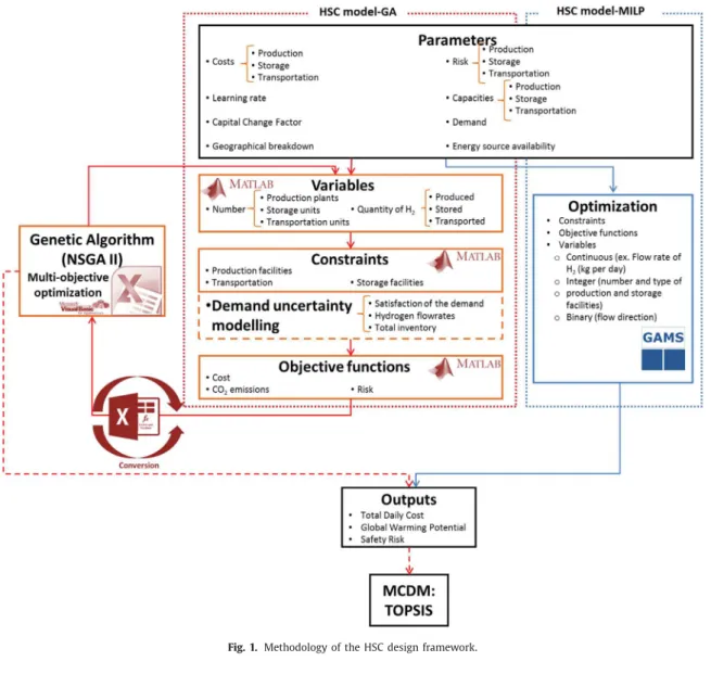
The general methodology of the HSC design proposed in this work is illustrated in Fig.1. It shows the extended flow diagram of the methodology proposed for HSC design optimization, considering both the multi-objective optimization framework either based on the deterministic MILP solution strategy developed in ( DeLeón

Almaraz, 2014) or on a GA and the multiple criteria decision mak-

ing tool selected to find the most interesting solution from the compromise solutions obtained from the Pareto front based on a variant of the TOPSIS method ( Ren et al., 2007). The MULTI- GEN environment previously developed in our research group [8] was selected as the genetic algorithm platform. The demand uncertainty has been modelled using fuzzy concepts as presented in ( Verdegay,1982, Villacortaetal.,2017).

2.2. CapturingtheHSCdesignmodelinaGAenvironment

The mathematical model previously developed by ( DeLeón

Al-maraz, 2014) for HSC design was solved within the GAMS 23.9

environment using CPLEX solver. This model has been adapted to be embedded in an external optimization loop based on the multi-objective genetic algorithm. The whole model is presented to maintain its integrity, and the changes that have been adopted to consider the integration into the external optimization loop are presented in italics.

2.2.1. HSCmodellingprinciples

A general supply chain network (SCN) model for hydrogen (see Fig.2) is considered (production plants, storage units, distribution grids and demand for each grid).

The following assumptions have been made: - The number of grids is known (8);

- The capacity of the production plants and the storage plants is known;

(6)

Fig. 1. Methodology of the HSC design framework.

(7)

Table 2

Optimization variables and dependent variables. Optimization variables Dependent variables

NP pig AH ig GC PGWP TCC NSs ig DI ig GWP Tot PT ig TDC PR pig DL ig LC RP ig TGWP Q ilgg’ FC MC SGWP FCC NTU ilgg’ SP ig FOC PD ig ST ig

- The demand for each one of the grids is fixed and known (for the crisp model);

- It is possible to either import or export hydrogen from/to each grid;

- Each grid can produce hydrogen in three different ways, i.e., steam methane reforming (SMR), electrolysis (centralized) and distributed electrolysis (decentralized, i.e., produced onsite for captive uses); and

- The average distance between the main cities is considered to calculate the delivery distances over the road network.

The mathematical model formulation involves the following no- tations:

- g and g’: grid squares such that g’ 6 = g(8) - i : product physical form (LH 2)

- l : type of transportation modes (tanker truck)

- p : plant type with different production technologies (SMR, electrolysis, diselectrolysis)

- s : storage facility type with different storage technologies (LH ₂ stock)

- e : energy source type (natural gas, solar, wind, hydroelectric, nuclear)

The model formulation is developed in the Appendix. The design decisions are based on the number, type, capacity, and loca- tion of production and storage facilities, the number of transport units, and the flow rate of hydrogen between locations. The op- erational decisions concern the total production rate of hydrogen in each grid, the total average inventory in each grid, the demand covered by imported hydrogen and local production.

The involved constraints are related to demand satisfaction, the availability of energy sources, production facilities, storage units, transportation modes and flow rates.

The variables used in this model are split into two groups: decision variables that are generated by the optimization procedure; and dependent variables that are calculated from the equality constraints. The classification is shown in Table2.

2.3. Multi-objectiveoptimizationbyGAs

The solving method used in this investigation is based on a multi-objective genetic algorithm. Let us recall that, in a single- objective optimization, the optimal solution is usually clearly defined. However, this assumption is not the case for a multi- objective problem in which the objectives can conflict. A single solution is hardly the best for all of the objectives simultaneously. Instead of a single optimum, there is a set of trade-off solutions, which are the so-called Pareto optima solutions. The aim of the multi-objective evolutionary algorithm is to cause the solution set

to approach the Pareto ideal frontier of the problem with a wide and uniform distribution in a single simulation run.

A variant of the non-dominated sorting genetic algorithm II (NSGA-II) ( Debetal.,2002), which is one of the most widely used multi-objective evolutionary algorithms implemented through the MULTIGEN library developed by ( Gomezetal.,2008), was selected in this work.

The main feature of NSGA-II among multi-objective evolutionary techniques is the determination of individual fitness values based on the Pareto dominance relationship and density informa- tion between individuals.

In this work, the results obtained from the

ε

-constraint method

( DeLeónAlmaraz,2014) and GA are compared to analyse the ad-

vantages and disadvantages of each technique and its impact on the network configuration of the HSC. The set of chromosomes representing the variables is illustrated in Fig.3.

The variable PR represents the production rate of product i by plant type p in grid g; Q is the flow rate of product i by transport l between the grids g and g’. NP is the number of production plants of type p of product i in grid g, while NS is the number of storage facilities of type p of product i in grid g. Finally, DL is the demand satisfied for product i by local production in grid g. In the GA used, the chromosome of the variables is complemented by a vector containing the type of variable (i.e., 0 for continuous variables, 1 for integer variables and 2 for binary variables). The other procedures follow the NSGAII variant proposed by ( Gomez etal., 2008).

2.4. Multiplecriteriadecisionmaking(MCDM)

A modified TOPSIS (M-TOPSIS) evaluation is based on the original concept of TOPSIS (technique for order of preference by similarity to ideal solution) and proposed by ( Renetal.,2007) is used. It chooses an alternative that should simultaneously have the closest distance from the positive ideal solution and the farthest distance from the negative ideal solution, solving the rank reversal and the evaluation failure problem presented in the original TOPSIS technique.

2.5. Uncertaintymodelling 2.5.1. Fuzzy-constraintproblems

The review proposed by ( Ebrahimnejad and Verdegay, 2016) has reported that many works have been devoted to fuzzy linear programming (FLP) and solution methods. These works are typically divided into four areas: (FLP1) linear programming (LP) problems with fuzzy inequalities and crisp objective function; (FLP2) LP problems with crisp inequalities and fuzzy objective function; (FLP3) LP problems with fuzzy inequalities and fuzzy objective function; and (FLP4) LP problems with fuzzy parameters. In the HSC design problem that has been mathematically formulated

( DeLeónAlmaraz,2014), hydrogen demand has been identified as

an uncertain parameter, and the HSC design problem refers to the simplest form of fuzzy linear programming, i.e., FLP1.

The decision maker can accept a violation of the constraints up to a certain degree previously established. This acceptance can be formalized for each constraint as ( Villacortaetal.,2017):

aix≤fbi,i=1,...,m

(8)

6

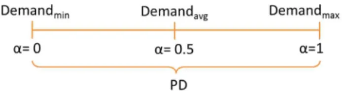
Fig. 4. Uncertain demand modelling.

In this expression, the f index indicates that the inferior relationship involves fuzzy numbers.

This index can be modelled using a membership function:

µ

i:R→[0,1],

µ

i

(

x

)

=

(

₁ _{i f}_x_≤_b i fi

(

x

)

i fbi≤x≤bi+ti

0 i fx≥bi+ti

where the f_i are continuous, non-increasing functions. The tolerance that the decision maker is willing to accept up to a value of

bi+ ti is given by the membership function

µ

i. For every x ∈ R,

µ

i( x) represents the degree of fulfilment of the i- th constraint.

Then, the problem can be solved: maxz=cx

subject to Ax≤fb x≥0

The approach proposed by ( Verdegay,1982) through the representation theorem has proved that the problem can be solved via the following parametric linear programming problem:

maxz=cx subject to Ax≤g

(

α

)

x≥0,

α

∈[0,1]

where g

(

α

)

=

(

g₁

(

α

)

, . . . , gm

(

α

)

∈ Rm, with gi= f_i−1.

To simplify the problem, if fiare linear: maxz=cx

subject to Ax≤b+t

(

1−

α

)

x≥0,

α

∈[0,1]

with t =

(

t1, . . . , tm

)

∈ Rm.

It has been proved ( Delgadoetal.,1993) that, when f_iis linear, a solution for the fuzzy constraints problem can be found as if it is a model with non-linear functions, without any generality loss when assuming linear functions for the fuzzy constraints. Some sample values can be applied to

α

in the interval [0,1], and then the model can be solved for every sample value. For example, a step size of 0.25 for sampling

α

can be transformed in five

α

-cuts for

α

=

{

0 ;0 . 25 ;0 . 5 ;0 . 75 ;1

}

.

2.5.2. ApplicationtodemanduncertaintymodellinginHSCNdesign

Hydrogen demand is the only parameter that will be considered uncertain. In this paper, only the modifications implemented in the HSC model are presented (see Fig.4).

The uncertainty has been considered using the following infor- mation:

- The lower and upper levels of demand have been obtained from the analysis in ( DeLeónAlmaraz,2014);

- From these values, average demand is calculated;

- The difference between the average and the low/high demand is calculated, representing an accepted tolerance; and

- Variable

α

is then introduced. This variable can take values from 1 to 0, and it represents the rate of use of tolerance. A value of

α

equal to 0.5 corresponds to the average demand. The constraints that are modified in the initial crisp version of the model are constraints 2-4.

Considering the demand as the right side of the constraints, as in Verdegays’ approach ( Verdegay,1982), the fuzzy right side can be expressed mathematically as:

g

DTig=

£

DTig+PDig

(

1−

α

)

¤

₍₁₎

Eq.(1)must be inserted into constraints (2)-(4), which replace the corresponding ones in the initial model (see ( De León

Al-maraz,2014)). DLig+DIig=DTig+PDig

(

1−

α

)

∀

i,g (2) PTig− X l,g′

¡

Qilgg′−Qilgg′g

¢

=DTig+PDig

(

1−

α

)

∀

i,g (3) STig

β

=DTig+PDig

(

1−

α

)

∀

i,g (4)

PD_ig is the tolerance of DT_ig, and

α

is the rate of use of the tolerance. Six values of

α

-cuts were considered:

α

=

{

0 . 16 ;0 . 33 ;0 . 5 , 0 . 66 ;0 . 83 ;1

}

. For each value of

α

-cuts, an evaluation of the model was performed.

3. Casestudy

3.1. ParametersoftheHSC

3.1.1. Estimationofhydrogendemand

The case study refers to the design for an HSC in the former Midi-Pyrénées region in France as previously presented in

( De León Almaraz, 2014). The demand is considered determin-

istic for the first case and is calculated from the work of

( McKinsey&Company, 2010) with the same methodology as pro-

posed in ( De-León Almaraz et al., 2014). The demand evolution profile corresponds to the values of D _min ( Table 3) (low demand scenario studied in ( De-León Almaraz etal., 2014)). The demand (for both D _min and D max) includes fuel cell electric vehicles and

captive fleets (i.e., buses, private and light-goods vehicles, forklifts) as defined in ( De León Almaraz, 2014). The market demand scenarios are established from ( Bento,2010) and ( McKinseyand Com-pany 2010), in which the two scenarios identifying the two levels of demands for FCEV penetration were developed providing the

Table 3

Demand scenarios of FCEV penetration.

Scenario/year 2020 2030 2040 2050

D min 1% 7.5% 17.5% 25%

(9)

Table 4

Demand (D min , D max ) and tolerance (PD) evolution profile used in the case study (kg per day).

Period/Grid 1 2 3 4

Dmin Dmax PD Dmin Dmax PD Dmin Dmax PD Dmin Dmax PD

2020 502 995 493 843 1650 807 977 1953 976 709 1404 695

2030 3780 7440 3660 6320 12430 6110 7410 14630 7220 5320 10450 5130

2040 8850 17350 8500 14750 29030 14280 17330 34100 16770 12400 24380 11980

2050 12610 24790 12180 21100 41470 20370 24770 48730 23960 17710 34810 17100

Period/Grid 5 6 7 8

Dmin Dmax PD Dmin Dmax PD Dmin Dmax PD Dmin Dmax PD

2020 570 1136 566 639 1263 624 3221 6362 3141 437 810 373

2030 4420 8590 4170 4850 9510 4660 24180 47670 23490 3150 6250 3100

2040 10260 20030 9770 11310 22160 10850 56470 111230 54760 7420 14570 7150

2050 14610 28610 14000 16170 31660 15490 80620 158950 78330 10580 20790 10210

percentage of FCEV expected to replace ICEs (ignition combustion engines).

The hydrogen demand for the two scenarios is obtained from

Eq.(5)( AlmansooriandShah,2006), ( MurthyKondaetal., 2011):

DTig=

(

FE

)

(

d

)

(

Qcg

)

(5)

where the total demand in each grid ( DT) is provided by the fuel economy of the vehicle ( FE), the average distance travelled ( d) and the number of FCEVs in each grid ( Qc).

For uncertain demand, Table4also presents the demand in the high demand scenario case proposed by ( De-León Almarazet al., 2014), i.e., (D max). The tolerances are represented by the differences

between D maxand D minover the periods.

3.1.2. Techno-economicassumptions

The study is based on the following assumptions:

- a capital change factor (depreciation period) of 12 years is introduced;

- in a multi-period approach, four periods were analysed, from 2020 to 2050, with a 10-year time step for each;

- three types of technologies to produce hydrogen are considered: steam methane reforming (SMR), electrolysis and distributed electrolysis;

- five energy sources are considered: solar, wind, hydro, nuclear and natural gas ( OchoaRoblesetal.,2018);

- hydrogen must be liquefied before being stored or distributed; - a minimum capacity of production and storage equal to 50 kg

of H ₂ per day is considered;

- renewable energy is directly used on site because of grid satu- ration, which allows to allocate the CO 2impact on each source;

- one size for storage and production units is considered; - inter-district transport is allowed;

- the maximum capacity of transportation is fixed at 3500 kg liquid-H ₂( Dagdouguietal.,2012);

- the hydrogen is stored in liquid form, and a 10-day LH ₂safety stock is considered;

- the risk index is calculated by the methodology proposed by

( KimandMoon,2008);

- the number of plants is initialized at a null value;

- the cost of switching from a current refuelling station to H 2fuel

is not considered; and

- the learning rate cost reductions due accumulated experience is considered as 10% per period ( McKinseyandCompany2010).

3.2. Optimizationparameters

For the mono-period and mono-objective case, a total of 500 individuals in the population and 10 0 0 generations are considered, with 0.9 for the crossover rate and 0.5 for the mutation rate. These values have been fixed from a preliminary sensitivity analysis. As already highlighted, the definition of variables is different in both models. In the GA formulation, there are 352 decision variables versus 676 in the MILP formulation. In the case of multi-period and multi-objective formulations, 20 0 0 individuals in the population and 30 0 0 generations are used, with 1408 variables versus 3319 in the MILP model. For the M-TOPSIS analysis ( Renetal.,2007), the same weighting factors for cost, safety, and environmental criteria are considered.The default feasibility of CPLEX and the optimality tolerances of 10 −6_{have been adopted.}

4. Results

In Sections4.1to 4.3, the same cost data as those used in (

De-LeónAlmarazetal.,2014) are adopted for validation purposes. The

parameters of the HSC model are presented in the supplementary materials. In all of the maps provided, the number of plants is in- dicated inside the symbols used for technology representation. The maps are obtained after the successive use of the optimization algorithm and the MCDM strategy for the multi-objective case.

For the mono-period optimization runs ( Sections4.1and 4.2), the demand scenario relative to period 4 is analysed.

4.1. Mono-objectiveandmono-periodoptimization

A preliminary study was performed with the GA approach: 10 runs were performed for each case to guarantee the stochastic nature of the algorithm ( Table5). The same methodology is used for all of the cases in which the GA methodology is used.

Table 5

Statistical results of the runs performed in the mono-period and mono-objective GA approach.

Min (TDC) Min (GWP) Min (Risk)

TDC (M$/ day) GWP (ton CO 2

eq / day) Risk TDC (M$ / day) GWP (ton CO eq per day) 2 Risk TDC (M$ / day) GWP (ton CO eq / day) 2 Risk

Mean 1.21 1552.08 496 1.32 763.42 485 1.22 1642.82 479

(10)

Table 6

Mono-objective and mono-period detailed optimization results.

The results of the three mono-objective optimizations (min TDC, GWP, and Risk separately), solved by CPLEX, on the one hand, and by the GA, on the other hand, are presented in Table6. For each criterion to be optimized, each column presents the optimized values of the decision variables, some intermediate values involved in the evaluation of the criteria and the optimized value of the considered criterion (in bold type and in colour). For each mono-optimization case, a computation of the other criteria is also performed in parallel.

Table6also presents the unit cost of H ₂ as well as the amount

of emitted CO ₂ per kg of H ₂ that is deduced from the value of the optimization criteria (in the same colour).

It can be observed that, whichever criterion is considered, CPLEX outperforms GA.

For instance, when TDC is minimized, a lower value is not sur- prisingly obtained with CPLEX (1.18 M$/day) than with GA (1.21 M$/day), which is exactly the same trend with the other criteria.

Let us consider once more the TDC case minimization for the sake of illustration. Since a better value has been obtained with MILP for TDC, the value of GWP is now higher than that obtained with GA (respectively, 10.82 kg CO 2-eq per kg H 2with MILP vs 7.83

kg CO 2-eq per kg H 2with GA), reflecting a compromise among the

criteria. This type of observation is not valid in this case for the risk criterion, which can be explained by different use of transport between the grids.

The trend observed for TDC can be generalized to the other criteria: it means that, if a better value is systematically obtained with MILP than with GA for a given criterion that has been optimized, the performance of one criterion that is not optimized can be degraded compared to the results obtained with GA in the same conditions.

Fig. 5 shows the obtained network for the three optimization cases. For TDC minimization, the networks obtained are very close to each other with both optimization strategies, producing the most hydrogen via SMR with some electrolysis plants. The main

difference between the approaches mostly involves the way in which hydrogen is distributed through the grids.

When GWP is minimized, priority is given to the production of hydrogen via electrolysis for both approaches. With the MILP model, there is no transport between grids, and hydrogen production is achieved through several distributed plants. With GA, fewer facilities are installed, but hydrogen transportation occurs through grids.

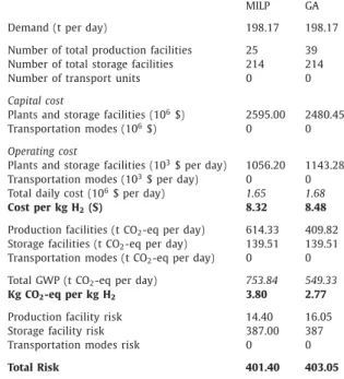
Table 7

Best trade-off solutions selected by TOPSIS for ε-constraint and AG.

MILP GA

Demand (t per day) 198.17 198.17

Number of total production facilities 25 39

Number of total storage facilities 214 214

Number of transport units 0 0

Capital cost

Plants and storage facilities (10 6_$) _2595.00 _2480.45

Transportation modes (10 6_$) ₀ ₀

Operating cost

Plants and storage facilities (10 3 $ per day) _1056.20 _1143.28

Transportation modes (10 3 $ per day) ₀ ₀

Total daily cost (10 6_{$ per day)} _1.65 _1.68

Cost per kg H 2 ($) 8.32 8.48

Production facilities (t CO 2 -eq per day) 614.33 409.82 Storage facilities (t CO 2 -eq per day) 139.51 139.51

Transportation modes (t CO 2 -eq per day) 0 0

Total GWP (t CO 2 -eq per day) 753.84 549.33

Kg CO 2 -eq per kg H 2 3.80 2.77

Production facility risk 14.40 16.05

Storage facility risk 387.00 387

Transportation modes risk 0 0

(11)

(12)

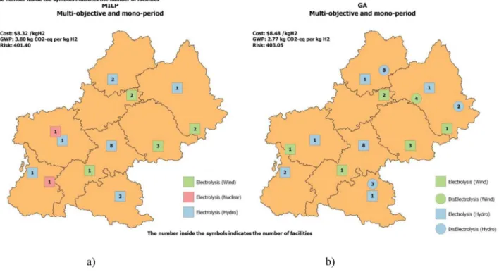
Fig. 6. Maps of the two scenarios with multi-objective optimization a) with GA; b) with MILP.

For risk minimization, hydrogen production is based exclusively on SMR plants for the MILP approach and a mix of SMR and electrolysis for the GA approach with transportation through grids. This situation is mainly due to the small difference in the risk values between the various technologies for the plant size that is considered.

It must be emphasized that the solar source is eliminated in the optimization process since hydrogen produced via electrolysis with solar energy is the most expensive process and exhibits a higher carbon footprint, compared to wind and hydro.

4.2. Multi-objectiveandmono-periodoptimization

In this case, the obtained results are only slightly improved with linear programming, compared to GA for cost and risk criteria

( Table7, Fig.6(a) and (b)). The degree of centralization is almost

the same. In Fig.6 (a), relative to GA, the configuration involves a set of several plants with the distributed electrolysis technology with no transportation; with MILP in Fig.6(b), priority is given to electrolysis plants from various sources, including the nuclear one (see Table8).

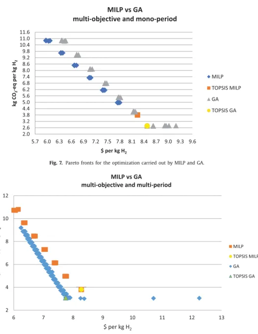
The Pareto solutions proposed by the GA include the Pareto space, which was identified as using the MILP methodology ( Fig.7). A small variation (2%) is observed in the unit cost ($8.32 of MILP vs $8.48 per kg H 2of GA) between the two TOPSIS solutions.

From the environmental viewpoint, a significant improvement is observed with the GA: GWP expressed in kg CO 2 eq per kg H 2 in

the GA approach is 27% lower than the value obtained with the Table 8

Use ratio of energy sources for hydrogen production (multi- objective and mono-period case).

Energy source MILP GA

Wind 60% 69%

Hydraulic 32% 31%

Nuclear 8% 0%

MILP approach. This difference can be explained by the use of distributed plants instead of electrolysis plants. The difference in the risk criteria between the approaches is not significant.

The computation time for MILP with CPLEX (Intel R

°

Xeon R

°

CPU 2.10GHz) is approximately 3 hours versus 4 hours with GA, with a set of 174 Pareto points obtained with the GA approach and 43 with the MILP approach.

4.3.Multi-objectiveandmulti-periodoptimization

Fig. 8 is a projection of the Pareto surface onto the two- dimensional plane corresponding to cost and environmental impact. For these two criteria, better compromise solutions are obtained with the GA than with CPLEX. This case is not true with the risk index, which can be higher.

The TOPSIS solutions (see Table9) provide lower values for both cost and GWP. The unit cost of hydrogen is lower with GA (8.00) than with MILP (8.27), despite a slightly higher risk (838 vs 873). This outcome can be explained by the way in which the plants are distributed through the periods.

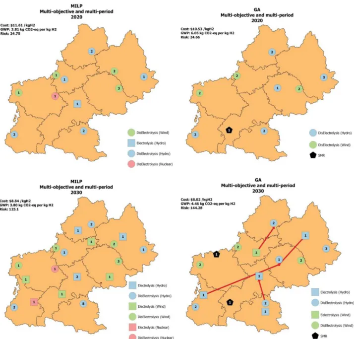
In the MILP approach ( Fig.9), priority is given in the first period to the establishment of distributed plants, mainly due to the low value of the demand. In the three other periods, the demand is satisfied mainly with the electrolysis plants so that GWP and risk remain not as high.

In the GA approach ( Fig.9), the first period is dedicated to the installation of distributed electrolysis plants and one SMR, signifi- cantly increasing CO 2emissions. For the second period, some elec-

trolysis plants are added. The CO ₂ emissions remain higher than with MILP, and because of transport between grids, the risk also increases. For the third and fourth periods, transport between grids remains, but the SMR plants disappear from distribution, decreas- ing the CO ₂emissions.

Finally, for this example and without providing a feature of generality to the obtained results, compared to MILP, GA promotes the deployment of hydrogen by favouring cost objectives in the first period. In the last two periods, better values for GWP are obtained with the GA approach rather than with MILP because of the instal-

(13)

Fig. 7. Pareto fronts for the optimization carried out by MILP and GA.

Fig. 8. Projection of the Pareto fronts onto the two-dimensional plane corresponding to cost and environmental impact for the optimization run carried out by MILP and GA for a multi-objective and multi-period approach.

lation of a smaller number of production facilities. This approach leads again to the implementation of transport between grids to satisfy the demand. Finally, from the safety point of view (risk), the MILP model presents better results, mostly due to the absence of transport between the grids. Table10shows the percentage of energy sources used by each methodology. Regarding the mono- objective case, the solar source is eliminated in the optimization process.

4.4. Multi-objectiveandmulti-periodoptimizationwithnewcosts

In addition to hydrogen demand, one of the most significant parameters is feedstock cost ( OchoaRoblesetal.,2017), ( Ochoa Rob-les et al., 2017). In the original model ( De-León Almaraz et al., 2014), the unit production cost (UPC) of electricity remains fixed for all of the periods regardless of the technology, which was a severe simplification. In what follows, an evaluation of UPC is considered with fixed facility costs (maintenance, labour cost), as well as electricity and feedstock costs.

Table 11presents the price of electricity produced from differ-

ent energy sources and the price of natural gas for conditions in France (2013).

In the original model, UPC is a fixed parameter ( De León

Al-maraz, 2014) (SMR: $3.36 per kg; electrolysis: $4.69 per kg; dis-

electrolysis $6.24per kg), which is only dependent on the size of the production unit ($ per kg H ₂). However, as mentioned in the

( McKinsey&Company,2010) report, a better vision of UPC is to con-

sider the fixed, electricity and feedstock costs. The fixed cost is related to labour and maintenance.

All of the contributions are reflected in Eq.(6), where the UPC calculation ($ per kg H 2) is given by the addition of the fixed cost

of a production plant of type p and size j in time period t (FCP ept,

$ per kg H ₂), the electricity cost for general usage in a production plant of type p projected for time period t (EC ept, $ per kg H 2) and

the feedstock e cost for a production plant of the p type (FSC ept).

The FSC ept is obtained by multiplying the feedstock e efficiency in

the process p in time t (kWh _elec/kg H 2) by the feedstock e price

(14)

Table 9

Multi-objective and multi-period optimization results.

MILP GA

Year 2020 2030 2040 2050 2020 2030 2040 2050

Demand (t per day) 7.90 59.43 138.79 198.17 7.90 59.43 138.79 198.17

Number of total production facilities 17 34 47 69 17 28 30 41

Number of total storage facilities 12 66 150 214 12 66 150 214

Number of transport units 0 0 0 0 0 4 2 3

Capital cost

Plants and storage facilities (10 6_$) _681.01 _765.69 _707.92 _185.42 _737.93 _520.31 _443.72 _153.42

Transportation modes (10 6 $) ₀ ₀ ₀ ₀ ₀ _0.80 _0.28 _0.41

Operating cost

Plants and storage facilities (10 3_{$ per day)} _49.35 _321.64 _748.23 _1066.00 _48.14 _332.99 _786.41 _1133.53

Transportation modes (10 3_{$ per day)} ₀ ₀ ₀ ₀ ₀ _1.31 _0.46 _0.46

Total daily cost (10 3 $ per day) _91.68 _525.60 _1127.00 _1600.25 _83.17 _476.53 _1116.65 _1557.90

Cost per kg H 2 ($) 11.61 8.84 8.12 8.08 10.53 8.02 8.05 7.86

Production facilities (t CO 2 -eq per day) 24.58 185.23 430.25 613.33 42.20 220.70 287.02 409.82

Storage facilities (t CO 2 -eq per day) 5.56 41.84 96.71 139.51 5.56 41.84 97.71 139.51

Transportation modes (t CO 2 -eq per day) 0 0 0 0 0 2.60 2.19 1.44

Total GWP (t CO 2 -eq per day) 30.14 226.07 526.96 752.84 47.76 265.13 386.91 550.77

Kg CO 2 -eq per kg H 2 3.81 3.80 3.79 3.79 6.05 4.46 2.79 2.78

Production facility risk 4.05 6.30 12.45 16.05 3.96 4.68 9.60 13.50

Storage facility risk 20.7 118.8 272.7 387 20.7 118.8 272.7 387

Transportation modes risk 0 0 0 0 0 20.8 6.5 14.3

Total Risk 24.75 125.10 285.15 403.05 24.66 144.28 288.80 414.80

Global TDC (M$ per day) 3.34 3.23

Global unit cost ($ per kg H 2 ) 8.27 8.00

Global GWP (T CO 2 eq per day) 1536 1251

Global Kg CO 2 -eq per kg H 2 3.80 3.09

Global Risk 838 879

Table 10

Use ratio of energy sources for hydrogen production (multi-objective and multi-period case).

Energy source MILP GA

2020 2030 2040 2050 2020 2030 2040 2050 Natural gas 0% 0% 0% 0% 6% 11% 0% 0% Hydro 53% 71% 70% 64% 53% 67% 70% 64% Wind 41% 24% 30% 36% 41% 22% 30% 36% Nuclear 6% 6% 0% 0% 0% 0% 0% 0% Table 11

Prices of natural gas and costs of electricity from different sources (2013).

Energy source (Price/unit) 2020 2030 2040 2050 Reference

European price of natural gas ($2010/kg) 0.587 1.300 1.750 ∗ _2.200 _{For 2030 and 2050: [48]}

Cost of electricity (nuclear) in France

( $2013/kWh ) 0.0439 0.0665 0.089

∗ _0.112∗ _{For 2020: [49]}

For 2030: [50] Cost of electricity (PV) in France ( $2013/kWh ) 0.328 0.101 0.060 ∗ _0.053 _{For 2020: [49]}

For 2030 and 2050: [51] Cost of electricity (Wind) in France ( $2013/kWh ) 0.073 0.068 ∗ _0.063∗ _0.058 _{For 2020: [49]}

For 2050: [51] Cost of electricity (Hydro) in France ( $2013/kWh ) 0.018 0.044 ∗ _0.071∗ _0.098

∗ _{Calculated by interpolation.}

ered is electricity, and the energy source cost varies depending on the type, e.g., fossil vs renewable ( Table11).

UPCe,p,t=FCPe,p,t+ECe,p,t+FSCe,p,t (6)

The feedstock cost is likely to gain importance because it depends on the energy transition scenario and induces a cost change in renewable energy impacting the hydrogen cost over the long- time horizon from 2020 to 2050.

The new UPC calculated for the model is presented in Table12, in which hydrogen produced via electrolysis with solar energy is

the most expensive, while hydrogen produced with electrolysis from a hydraulic source is less expensive.

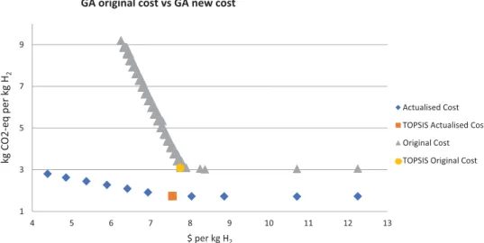
The optimization runs are performed with these new costs, and the results are compared with the previous ones (see Fig. 10). A strong decrease in GWP is observed for the range of these new costs, globally leading to better solutions for all criteria.

In the first period (see Fig. 11 and Table 13), the distributed plants are the main sources of production, while in the other periods, the electrolysis plants started to be installed in the different grids. Additionally, there is no transport between grids, and the CO 2 emissions for the plants installed remain very low. Most of

(15)

Fig. 9. Maps of the four scenarios for the optimization run carried out by MILP and GA for a multi-objective and multi-period approach.

Table 12

UPC calculated with the new costs. Production technology Fixed cost of production ($ per kg H 2 ) Electricity usage of production plant ($ per kg H 2 ) Feedstock cost for production plant ($ per kg H 2 ) Electrical need to produce a kg of H 2 kWh elec /kg H 2

Cost of energy source ($ per kg H 2 ) ∗ UPC ($ per kg H 2 )

2020 2030 2040 2050 2020 2030 2040 2050 SMR 0.16 0.02 4.02 ¥ _3.71 _2.61 _3.46 _4.62 _3.89 _2.79 _3.64 _4.80 Electrolysis PV 0.39 0.06 55 18.04 5.56 3.30 2.93 18.49 6.01 3.75 3.38 Wind 0.39 0.06 55 4.00 3.72 3.45 3.17 4.45 4.17 3.90 3.62 Hydro 0.39 0.06 55 0.98 2.44 3.90 5.36 1.43 2.89 4.35 5.81 Nuclear 0.39 0.06 55 2.41 3.66 4.90 6.14 2.86 4.11 5.35 6.59 Dis Electrolysis PV 0.75 0.11 55 18.04 5.56 3.30 2.93 18.90 6.42 4.16 3.79 Wind 0.75 0.11 55 4.00 3.72 3.45 3.17 4.86 4.58 4.31 4.03 Hydro 0.75 0.11 55 0.98 2.44 3.90 5.36 1.84 3.30 4.76 6.22 Nuclear 0.75 0.11 55 2.41 3.66 4.90 6.14 3.27 4.52 5.76 7.00

∗_{[Energy source cost ($/KWh)x Electrical need to produce a kg of H}

2 (kWh elec /kg H 2 )].

(16)

Fig. 10. Pareto fronts obtained with the original GA and the GA with the new cost.

(17)

Table 13

Multi-objective and multi-period results for actualised costs. GA new costs

Year 2020 2030 2040 2050

Demand (t per day) 7.90 59.43 138.79 198.17

Number of total production facilities 25 62 92 110

Number of total storage facilities 12 66 150 214

Number of transport units 0 0 0 0

Capital cost

Plants and storage facilities (10 6_$) _304.47 _401.53 _263.71 _43.44

Transportation modes (10 6 $) ₀ ₀ ₀ ₀

Operating cost

Plants and storage facilities (10 3_{$ per day) 43.44} _307.15 _708.68 _1013.16

Transportation modes (10 3 $ per day) ₀ ₀ ₀ ₀

Total daily cost (10 3 $ per day) _80.12 _489.34 _1036.96 _1446.56

Cost per kg H 2 ($) 10.14 8.23 7.47 7.30

Production facilities (t CO 2 -eq per day) 8.27 61.35 142.51 201.91

Storage facilities (t CO 2 -eq per day) 5.56 41.84 97.71 139.51

Transportation modes (t CO 2 -eq per day) 0 0 0 0

Total GWP (t CO 2 -eq per day) 13.73 103.18 240.22 341.42

Kg CO 2 -eq per kg H 2 1.74 1.74 1.73 1.72

Production facility risk 7.20 9.00 12.45 20.55

Storage facility risk 20.7 118.8 272.7 387.0

Transportation modes risk 0 0 0 0

Total Risk 27.90 127.80 285.15 407.55

Global TDC (M$ per day) 3.05

Global unit cost ($ per kg H 2 ) 7.55

Global GWP (T CO 2 eq per day) 698

Global Kg CO 2 -eq per kg H 2 1.73

Global Risk 848

Table 14

Use ratio of energy sources for hydrogen production (with new costs).

Energy sources 2020 2030 2040 2050

Hydro 22% 30% 22% 33%

Wind 78% 70% 78% 67%

the energy sources used stem from wind, with almost 70% of the electricity produced ( Table14).

4.5. Multi-objectiveGAapproachunderuncertaindemand

In this case, the demand can vary between low and high demand (Dmin and Dmax, respectively, in Table4). The tolerance is

the difference between the two levels of demand, and

α

is the percentage of tolerance that is added to the base demand (Dmin). Sev- eral values of

α

are used (see Table15), and the demand used for each

α

-cut depends on the tolerance level.

For each

α

-value, a tri-criterion optimization procedure with the GA procedure is implemented, leading to the set of solutions constituting the Pareto front, to which the M-TOPSIS procedure is then applied. The criteria (average values over the periods) relative to the compromise solution of the HSCN finally obtained are presented in Table16, and the instances obtained for

α

equal to 0; 0.16; 0.33; and 0.50 are shown in Table 17, in which the relative deviation relative to the case

α

equal to 0 case is presented.

Table 15

(18)

Table 16

Results of HSCN solutions the different α-cuts (average values over the period).

Table 17

(19)

Table 18

Robustness analysis of the optimal configurations.

α= 0.33 α= 0.66 α= 1

2020 2030 2040 2050 2020 2030 2040 2050 2020 2030 2040 2050

TDC (M$ per day) 89.24 514.66 1083.21 1494.42 93.31 554.59 1193.17 1614.67 98.93 593.65 1292.13 1729.73

Relative deviation (reference α= 0) 11% 5% 4% 3% 16% 13% 15% 12% 23% 21% 25% 20%

Unit cost ($ per kg H 2 ) 11.30 8.66 7.80 7.54 11.81 9.33 8.60 8.15 12.52 9.99 9.31 8.73

relative deviation (reference α= 0) 11% 5% 4% 3% 16% 13% 15% 12% 24% 21% 25% 20%

GWP (T CO 2 eq per day) 13.83 103.19 240.22 341.42 13.85 103.51 241.02 341.98 13.74 102.96 240.52 341.55

relative deviation (reference α= 0) 0% 0% 0% 0% 0% 0% 0% 0% 1% 0% 0% 0%

GWP (kg CO 2 eq per kg H 2 ) 1.74 1.74 1.73 1.72 1.75 1.74 1.74 1.73 1.74 1.73 1.73 1.72

relative deviation (reference α= 0) 0% 0% 0% 0% 1% 0% 0% 0% 0% 0% 0% 0%

Risk 45.25 278.12 602.26 821.36 70.31 326.36 749.19 1064.64 94.76 373.11 764.79 1099.59

relative deviation (reference α= 0) 62% 118% 111% 102% 152% 155% 163% 161% 240% 192% 168% 170%

Fig. 12. Cost of hydrogen in 2050 ($ per kg H 2 ).

As expected, the operating cost and the capital cost increase with hydrogen demand. Although the TDC is higher when

α

increases, the unit cost decreases, mostly due to the effect of scale. For example, in the first period (2020), with a value of

α

equal to 0 (respectively 0.5), the unit cost of H 2 is $10.14/kg H 2(respec-

tively $6.98/kg H ₂). The same situation is observed over the whole period. Conversely, GWP and risk increase with hydrogen demand. The number of facilities also increases as

α

-value increases, ex- cept for

α

equal to 0.5, for which priority is given to electrolysis plants instead of distributed ones, allowing for greater capacity to be available.

A robustness study can thus be performed from the optimization results presented in Table18. Let us consider the HSCN configuration obtained with

α

equal to 0.33. The network, which has been obtained from the successive use of the multi-objective optimization procedures and MCDM techniques, is perfectly consistent with the corresponding demand. However, if the demand does not reach the maximal expected value, it will result in higher values for all criteria. To check whether an acceptable range for the criteria values can still be obtained even if the network is over- dimensioned for this demand level, a post-optimal analysis is then performed using the given network and the lowest value of the demand. Table18compares the results obtained in both scenarios.

4.6. Resultsanddiscussion

The hydrogen price evolution is directly dependent on production and distribution costs. The different studies have shown the

hydrogen cost evolution with the gradual introduction of demand from the mobility sector. A comparative study of the different results considering different FCV market penetration rates, considering different hydrogen production technology choices, was carried out, and even for the highest demand, the results show (see Fig. 12) that hydrogen costs for 2050 remain expensive compared to the Hyways roadmap targets ( European Commission 2008) for the best compromise solutions obtained using the proposed multi- objective-MCDM framework. For the sake of illustration, the best solution obtained for hydrogen cost minimization ($4.18/kg of H ₂) and GWP minimization ($7.30/kg H 2) has also been reported. A

consistent approach would be to find a compromise solution between these bounds since the GWP is consistent with the targeted values ( Mobilité HydrogèneFrance2016) (see Fig.13).

Fig.13 compares the well-to-wheel CO 2 emissions per km ob-

tained with FCEVs obtained by the use of the proposed methodology and those related to ICE vehicles equipped with gasoline- or diesel-fuelled engines ( HydrogenCouncil2017) for the 2050 period. Currently, on-road fuel economy is approximately 1 kg of hydrogen per 100 km travelled, and the emissions expected for ICE vehicles are approximately 60 g CO 2/km ( IEA2015). With the costs

used in the original models, the emissions are in the range of 28 - 38 g CO ₂/km for the MILP and GA approaches, respectively. With the new UPC cost, the emissions are less than 20 g CO 2/km. It must

be emphasized that FCEV emissions are expected to be less than 23 g CO ₂/km ( Mobilité Hydrogène France 2016) in 2030, which means that the HSCN obtained with the new costs is competitive with the expected results.

(20)

Fig. 13. Comparison of emissions by sector in 2050 (g CO 2 /km). Data from [59].

5. Conclusion

This paper has presented the core methodology for HSCN design, combining multi-objective optimization tools and multiple criteria decision-making techniques. The scientific challenge of this work was to use the potential of genetic algorithms as an alternative to the current methodologies in the optimization of the HSC design, particularly as a complementary approach to the MILP framework previously developed in ( De-LeónAlmarazetal.,2014): the size and particularly the number of binary variables have often led to difficulties for problem solution in ( De-León Almaraz et al., 2014). In this work, a variant of NSGA-II previously developed in ( Gomezet al., 2008) was explored to address the multi- objective formulation so that compromise solutions can be automatically produced.

The case study of the hydrogen mobility market in the former Midi-Pyrenées region has been considered since it was already studied in ( De-LeónAlmarazetal.,2014) for validation purposes of the proposed methodology: it is foreseen to be the fastest growing and most important market in the horizon of 2025 – 2030 and thus is clearly relevant to the context of a “green hydrogen” study. The objective functions obtained by GA exhibit the same order of magnitude as those obtained with MILP in the mono-criterion problem, and the multi-objective GA yields a Pareto front of better quality with a better distribution of the compromise solutions. However, in our view, both strategies do not have to be opposed, but the maximum use of their potential benefits must be made.

Several experiments were developed with a fixed demand and for mono- and multi-objective cases. In the multi-objective instances, the GA outperforms the

ε

-constraint strategy. It must be emphasized that the GA prioritizes the TDC cost, providing better results than the

ε

-constraint method, as well as the transportation of hydrogen between the grids. The differences in the distributions and the results between the GA and the MILP approaches can be explained by way of managing the constraints and their different logics.

In the original model ( De-LeónAlmaraz etal., 2014), the unit production cost (UPC) of electricity remains fixed for all of the periods, regardless of the hydrogen technology, which was a severe simplification. The unit production cost involves the fixed facility costs (maintenance, labour cost), as well as electricity and feedstock costs, which are more relevant to the reality of costs.

Hydrogen demand was identified as one the most significant parameters for HSCN design, and a GA model was developed with demand uncertainty modelled using fuzzy concepts.

Since hydrogen demand was simply involved through constraints in the HSCN model formulation, the HSC design problem refers to the simplest form of fuzzy linear programming, as proposed by ( Verdegay,1982), ( EbrahimnejadandVerdegay,2016,

Delgadoetal., 1993). The solution strategy can thus be easily im-

plemented by varying

α

, which can be considered the percentage of tolerance added to the base demand. This sensitivity analysis has allowed for identifying more robust solutions. The solutions are compared with the original crisp models, based on either MILP or GA, giving more robustness to the proposed approach.

An extension could be to develop a fuzzy optimization model for supply chain design that considers demand and price uncer- tainties. The model could be formulated as a fuzzy mixed-integer linear programming model, in which the data are poorly known and modelled by triangular fuzzy numbers. The synergetic effect of genetic algorithms and fuzzy demand modelling could be thus explored so that the fuzzy model would provide the decision maker with alternative decision plans for different degrees of satisfaction. Finally, this study has revealed that if the economic and environmental criteria can be formulated by proven methodologies, the safety risk is perhaps more difficult to formulate and calibrate.

The use of the framework could be useful in deploying hydrogen solutions since the introduction of hydrogen as an energy car- rier is not only a technology challenge, but it also requires the con- vergence of many economic, environmental and social factors.

DeclarationofCompetingInterest

All authors have participated in (a) conception and design, or analysis and interpretation of the data; (b) drafting the article or revising it critically for important intellectual content; and (c) ap- proval of the final version.This manuscript has not been submitted to, nor is under review at, another journal or other publishing venue.The authors have no affiliation with any organization with a direct or indirect financial interest in the subject matter discussed in the manuscript

Supplementarymaterials

Supplementary material associated with this article can be found, in the online version, at doi: 10.1016/j.compchemeng.2020.

(21)

Appendix

Indices

g and g’ Grid squares such that g’ 6 = g (8)

I Product physical form

L Type of transportation mode

P Plant type with different production technologies

S Storage facility type with different storage technologies

E Energy source type

Parameters

B Storage holding period - average number of days’ worth of stock (days)

γepj Rate of utilization of primary energy source e by plant type p and size j (unit resource/unit product)

AD gg’ Average delivery distance between g and g’ by transportation l (km per trip)

Adj gg’ Road risk between grids g and g’ (units)

CCF Capital change factor payback period of capital investment (years) DT ig Total demand for product form i in grid g (kg per day)

DW l Driver wages for transportation mode l (dollars per hour)

FE l Fuel economy of transportation mode l (km per litre)

FP l Fuel price of transportation mode l (dollars per litre)

GE l General expenses of transportation mode l (dollars per day)

GWProd p Production GWP by plant type p (g CO 2 -eq per kg of H 2 ) GWStock i Storage global warming potential form i (g CO 2 -eq per kg of H 2 ) GWTrans l Global warming potential of transportation mode l (g CO 2 per ton-km)

LUT l Load and unload times of product for transportation mode l (hours per trip)

ME l Maintenance expenses of transportation mode l (dollars per km)

NOP Network operating period (days per year)

Qmax il Maximum flow rate of product form i by transportation mode l (kg per day)

Qmin il Minimum flow rate of product form i by transportation mode l (kg per day)

PCapmax pi Maximum production capacity of plant type p for product form i (kg per day)

PCapmin pi Minimum production capacity of plant type p for product form i (kg per day)

PCC pi Capital cost of establishing plant type p producing product form i (dollars)

RP p Risk level of the production facility p (units)

RS s Risk level of the storage facility s (units)

RT l Risk level of the transportation mode l (units)

SCapmax si Maximum storage capacity of storage type s for product form i (kg)

SCapmin si Minimum storage capacity of storage type s for product form i (kg)

SCC si Capital cost of establishing storage type s storing product form i (dollars)

SP l Average speed of transportation mode l (km per hour)

SSF Safety stock factor of primary energy sources within a grid (%)

TCap il Capacity of transportation mode l transporting product form i (kg per trip)

TMA l Availability of transportation mode l (hours per day)

TMC il Cost of establishing transportation mode l for product form i (dollars)

UPC pi Unit production cost for product i produced by plant type p (dollars per kg)

USC si Unit storage cost for product form i at storage type s (dollar per kg-day)

W l Weight of transportation mode l (tons)

WFP g Weigh factor risk population in each grid (units)

Variables

A Rate of utilization of the tolerance AH ig Available hydrogen in grid g

DL ig Demand for product i in grid g satisfied by local production (kg per day)

DI ig Imported demand for product form i in grid g (kg per day)

FC Fuel cost (dollars per day)

FCC Facility capital cost (dollars)

FOC Facility operating cost (dollars per day)

GC General cost (dollars per day)

GWPTot Total global warming potential of the network (g CO 2 -eq per day)

LC Labour cost (dollars per day)

MC Maintenance cost (dollars per day)

NPp ig Number of plants of type p producing product form i in grid g

NSs ig Number of storage facilities of type s for product form i in grid g

NTUil gg’ Number of transport units between g and g’

PD ig Tolerance of the demand in grid g

PGWP Total daily GWP in production facility p (g CO 2 -eq per day)

PR pig Production rate of product i produced by plant type p in grid g (kg per day)

PT ig Total production rate of product i in grid g (kg per day)

Qil gg’ Flow rate of product i by transportation mode l between g and g’ (kg per day)

RP ig Received hydrogen in grid g

SGWP Total daily GWP in the storage technology s (g CO 2 -eq per day) SP ig Overproduction of hydrogen in grid g

ST ig Total average inventory of product form i in grid g (kg) TCC Transportation capital cost (dollars)

TDC Total daily cost of the network (dollars per day) TGWP Total daily GWP in transportation mode l (g CO 2 -eq per day) TOC Transportation operating cost (dollars per day)

TotalRisk Total risk of this configuration (units) TPRisk Total risk index for production activity (units) TSRisk Total risk index for storage activity (units) TTRisk Total risk index for transport activity (units)