Defect segmentation on 'Jonagold' apples using colour vision and a
Bayesian classification method
V. Leemans , H. Magein, M.-F. Destain
Faculté Universitaire des Sciences Agronomiques de Gembloux, Passage des Déportés, 2, B-5030 Gembloux, Belgium
Abstract
This paper shows how the information enclosed in a colour image of a bi-colour apple can be used to segment defects. A method to segment pixels, based on a Bayesian classification process, is proposed. The colour frequency distributions of the healthy tissue and of the defects were used to estimate the probability distribution of each class. The results showed that most defects, namely bitter pit, fungi attack, scar tissue, frost damages, bruises, insect attack and scab, are segmented. However, russet was sometimes confused with the transition area between ground and blush colour.
Keywords : Apple defects ; bi-colour fruit ; colour vision ; computer vision ; image segmentation
1. INTRODUCTION
The quality standards for apples issued by the European Union (Anonymous, 1989) specify three different categories based mainly on the external quality of the fruit, the presence of defects, their size and location. Fruit sorting automation according to these standards could be achieved by colour machine vision. This technique requires as a first step a defect segmentation.
Yang (1994) used a flooding algorithm on apples to segment 'patch-like' defects on monochrome images. This method did not require many assumptions about the grey level distribution but could be difficult to apply on bi-colour fruits where the defects are usually darker than the ground bi-colour, but lighter than the blush bi-colour. Molto et al. (1995) studied the external quality of different fruits including peaches, oranges apples and pears. The authors used linear discriminant analysis to segment pixels into three or four classes (peel, stain, stem or background). The accuracy was good for apples, excepted for the 'stem' class. A wider range of defects should however be taken into account. Leemans et al. (1998) used a Gaussian model of the colour to segment defects on 'Golden Delicious' apples, completed with two enhancement steps. The detection was effective, but revealed some noise (healthy tissue presenting patches and segmented as defect). Nakano (1997) studied the colour grading of 'San-fuji' apples, presenting a red surface colour and an orange to light green background colour. A first neural network was used to grade the pixels into six categories, 'normal red', 'poor red', 'injured', 'vine' and 'upper' or 'lower background' with an accuracy over 95%. A second neural network classified the whole surface of the fruit into 'superior', 'excellent', 'good', 'poor' and 'damaged'. The classification rate was 75% for the damaged fruits. All the mentioned authors who were working on colour images used the r, g, b colour space. The classification proposed used by Molto et al. (1995) and Nakano (1997) required a segmentation or selection of pixels by an operator while methods used by Yang (1994) and Leemans et al. (1998) did not, which is
advantageous.
This paper focuses on the defects segmentation of Jonagold apples which are bi-colour.
2. MATERIALS AND METHODS 2.1. The material
The image acquisition system is described in Leemans et al. (1998) and included a lighting tunnel, a three CCD colour camera (Sony XC003P, Brussel), a frame grabber (Imascan Chroma-Imagraph, Chelmsford, MA, USA) and a PC (Pentium 133 MHz, Santa Clara, CA, USA). The basic treatments were carried out using Image-Pro Software (Media cybernetics, Silver Spring, MD, USA) while the other algorithms were written in C + +. The
images were acquired with a resolution of 3.6 pix/mm2. In order to have execution times compatible with on-line
grading, the resolution was reduced to 0.9 pix/mm2 before segmentation. These images are 120 pixels width and
95 pixels height.
Two samples were used during this study. Sample 1 contained only healthy fruits and was subdivided into sub-sample 1a and 1b: 1a included 400 fruits (Jonagold apples) coming from an auction, the 'Belgische Fruit Veiling', in January 1997, equally shared into categories A3 + +, A3 +, A3 and A3r; 1b included 140 fruit in categories A2 + + , A2 + , A2, A2r, and out of category, overripe (coming from the same auction). Categories A are good quality fruits; A3 have at least 25% of blush area, while A2 have at least 33% of blush area; + + codes for far green ground colour, + for green ground colour," for normal ground colour and r for ripe (yellow) ground colour, according to Belgian standards. Each fruit was represented by four images, with the stem to calyx axis perpendicular to the camera optical axis. The first view was randomly chosen and the others were obtained by rotation of the fruit through 90°. The second sample contained the fruits presenting at least one defect. One image was acquired for each defect, with the defect presented to the camera. Sub-sample 2a included 42 of these images and sub-sample 2b 165 images. In all, 222 different defects were encountered as a result of: bitter pit, fungi attack, scar tissue, frost damage, bruises, insect attack, russet and scab.
Both sub-samples 1a and 2a were used for parameter fitting, while sub-samples 1b and 2b were used for the validation.
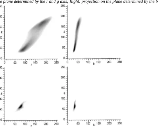
Fig. 1. Relative frequency diagrams. Upper: healthy tissue colours; Lower: defect colours. Left: projection on
the plane determined by the r and g axis; Right: projection on the plane determined by the b and g axis.
2.2. The method
Jonagold apples are characterised by a green ground colour and a darker red blush colour. The two upper graphs in Fig. 1 represent two projections of the relative frequency distribution of the healthy tissues' colours, on a plane determined, respectively, by the axis r-g (red green) and b-g (blue green); the position on the graph represents the colour, and the grey level is proportional to the relative frequency in each plane (a white level indicates a null relative frequency and the black level indicate the maximum relative frequency). This relative frequency
blue) co-ordinate (88, 45, 33) representing the blush colour and the other one around (181, 177, 55)
corresponding to the ground colour. The central area, representing the transition colours between the blush and the ground colour, was in a 'pass' between the two maxima, i.e. it had a lower frequency than the blush and ground colours. On the other hand, this filled a larger surface on the upper diagrams of Fig. 1. and so represents a wider range of different colours. The blush, intermediate and ground colours represented, respectively, 46%, 10% and 44% of the total numbers of the pixels belonging to the images. Of the 16 million available colours (a colour is coded by 8 bits in each r, g and b channel), 264182 represented the apples.
Preliminary tests showed that the segmentation process based on non-parametric colour models of the healthy tissue did not have enough accuracy. The segmentation of the defects was thus considered as a classification process of each pixel into 'healthy' or 'defect' classes based on the pixels' colours. Bayes's theorem gave the probability for a pixel to belong to the healthy tissue on its colour basis:
P(healthy|x) = P(x|healthy) x P(healthy)/P(x)
with x the (r, g, b) colour component vector; P(healthy|x) the a posteriori probability for the healthy tissue or the probability for a pixel having the colour x to belong to the healthy tissue; P(x|healthy) the probability for a pixel belonging to class 'healthy' to have the colour x; P(healthy) the healthy colour class a priori probability; P(x) the probability to observe the colour x (the two classes blended). The complementary probability was given by:
P(defect|x) = P(x|defect) x P(defect)/P(x)
with P(defect|x) the a posteriori probability for the defect or the probability for a pixel having the colour x to belongs to a defect; P(defect) was the defect colour class prior probability. As two classes were
considered:P(healthy|x) = 1-P(defect|x).
The pixel would be allocated to the classes with the highest probability, higher than 0.5.
Three independent parameters should be estimated: P(x|healthy), P(healthy) and P(x|defect). The a priori probabilities P(healthy) or P(defect) were unknown and variable in time (depending on the harvest condition, climate of the season,...) and space (depending on the grower, soil, local climate,...). Both prior probabilities were thus considered equal:
In this case, the pixel was graded taking into account an unknown threshold. The ratio of healthy pixels was clearly wider than those of the defect pixels. This threshold was thus comprised between 0 and 0.5, and was considered as a parameter of the model. The kernel method was used to estimate P(x|healthy) and P(x|defect). The colour of the fruit in sample 1 was used to compute the 'healthy tissue colour frequency distribution' (f(x)). The relative frequency distribution fr(x) was then computed:
fr(x) = f(x)/n,
with n the sample size. fr(x) is represented in Fig. 1 above. As the sample was considered representative for the fruit population, this distribution tends towards the corresponding probability distribution when n grows. The sample size is high (about 11 x 106) but it must be compared to the 264 000 colours representing the fruits. It was
observed that the maximum colour resolution was not required for the defect segmentation. The six most significant bits in each r, g, b channel were thus taken into account and the resulting amount of colour classes was reduced to 6 000. In that case the sample size seems high enough and several conditional colour frequency distributions were observed to validate this assumption. If the sample size is big enough, the random variations as a result of the sampling should disappear. Fig. 2 represents some of these conditional distributions, which were considered soft enough to represent the probability distribution: P(x|healthy) = fr(x).
The same distributions were also computed on the defect parts of the fruits in sample 2a (defect colour frequency distribution, fd(x)). The defects were segmented by the operator. A first way consisted in delimiting the defect by an irregular area of interest, using the mouse, and then colouring this area in blue (Image-Pro software, Silver Spring, MD, USA). The most difficult defects, such as the reticular russet, were painted in blue using Microsoft
Paint (Window 95 tools, Microsoft Corporation, Washington, USA). Then for both cases, applying a threshold on the blue channel and a logical bit AND operation gave an image of the defect on a black background. Another way to proceed consisted in using the colour recognition function implemented in Image-Pro. The segmentation of these defects by an operator required several days. This limited the sample size: about two 105 pixels and
about 2 500 classes. Nevertheless, the curves concerning the defects colours in Fig. 2 were also considered as soft enough. We had thus:
with frd the relative frequency distribution for the defect colours; nd the defect colour sample size, frd is represented in the lower part of Fig. 1.
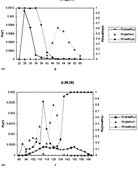
Fig. 2. Conditional probabilities P(x|healthy), P(x|defect) and a posteriori probability P(healthy)for several
colours.
It was also admitted that P(healthy|x) = 0 if both P(x|healthy) and P(x|defect) are null: the considered colour was never encountered, either for the defects or the healthy tissue. P(x|healthy), P(x|defect) and P(healthy|x) are represented in Fig. 2. Fig. 2a shows the relation between g and the three probabilities, for r = 62 and b = 22. This corresponds to the blush colour for the healthy tissue. P(x|healthy) and P(x|defect) do not overlap
themselves and the transition between P(healthy|x) = 1 and P(healthy|x) = 0 is neat. This is usually the case, but for several conditional distributions, the situation in Fig. 2b can be observed. Fig. 2b shows the same relation as
Fig. 2a but for g = 98 and b = 38, corresponding to the transition area. The curve representing P(x|defect) shows several maxima, which can also be noticed in Fig. 1, mainly on the r-g diagram. These maxima represent the different defects (scar tissue, rotten tissue, reaction to scab, fruit flesh, etc). The peak centred at r = 124 (Fig. 2b) corresponds to the russeting and is responsible for a drop for P(healthy|x). In Fig. 1, frd presented a smaller variability, filling a smaller area than fr. This explains why in Fig. 2 P(x|defect) is often higher than P(x|healthy). The computation of P(healthy|x) was made before the segmentation process and written in a look-up table. The segmentation consisted in comparison of the value of the look-up table at colour x (coded on six bytes) to the threshold. This process is rapid (5 ms for an image).
The local enhancement applied on Golden Delicious apples and described by Leemans et al. (1998) was also tested here. The size of the kernel was 7x7 pixels and the method was applied once. The duration of this step is 30 ms for an image.
The 42 images in set 2a were used to adjust threshold value.
3. RESULTS AND DISCUSSION
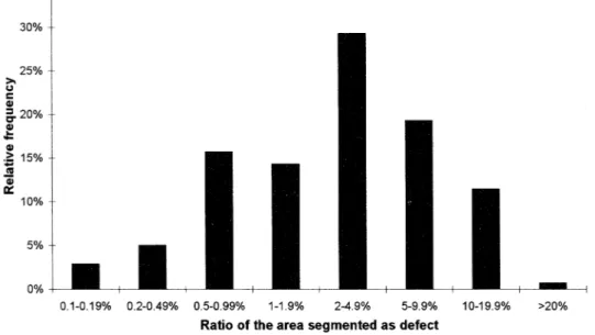
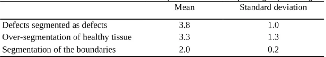
The 725 images in samples 1b and 2b were used to test the algorithms. Two separate methods were used to evaluate the results on the healthy fruits and the fruits presenting a damage. For the first ones (sample 1b), the ratio of the surfaces of patches erroneously segmented as defect to the whole surface of the fruit was measured for each image. These data are summarised in Fig. 3. It can be noticed that 69% of the healthy fruits have less than 5% of their surface segmented as defect, while 88% of these fruits have less than 10% of their surface segmented as defect. The confusion between healthy tissue and defect is possible mainly with russet. A fruit presenting a chaotic blush colour as in Figs. 4 and 2a, would thus be graded in category I instead of Extra. For the damaged fruits (sample 2b), the same quotation used by Leemans et al. (1998) was used here. Three marks were given for each image. The first one dealt with the accuracy in defect segmentation, ranging from 1 to 5: 5 for a correct detection compared with human assessment, 3 for minor differences, 1 for major differences. The second mark indicated how the healthy tissue was segmented as defect, also ranging from 1 to 5 (1 for a major area of healthy pixels segmented as defect; 5 for no good pixels segmented as defect). The third mark concerned the detection of the boundaries as defect, ranging from 1 to 3. Table 1 gives a summary of the quotations. The mean mark for the defect segmentation, 3.8, indicates a good segmentation efficiency. Only 4% of the image have their first mark below 3. The mean mark for the over-segmentation of healthy tissue is 3.3 and 22% of the images have the second mark below 3. This reveals an over-segmentation. The mean mark for the boundaries of the fruit indicates that the boundaries are generally segmented as defect, but as these areas are limited, they could be removed by erosion.
Table 1 : Mean marks and standard deviation for the evaluation of damaged fruit images
Mean Standard deviation
Defects segmented as defects 3.8 1.0
Over-segmentation of healthy tissue 3.3 1.3
Segmentation of the boundaries 2.0 0.2
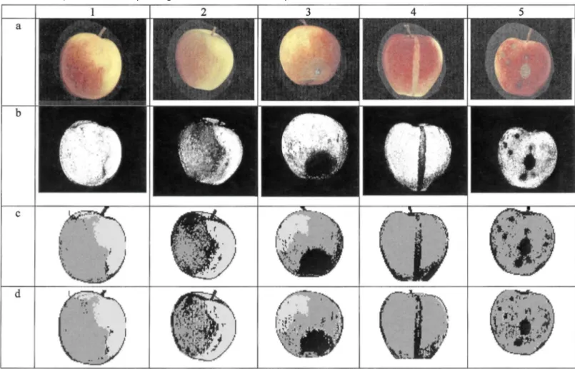
The discussion presented here will concern the whole set and is illustrated with the five images in Fig. 4, chosen to be representative of the method's results. The first row (a in Fig. 4) shows five original images. The green parts are the ground colour areas and the red parts are the blush colour. In the images on the second row (b), the probability P(healthy|x) is represented by the grey level: the maximum probability (equal to 1) appears in white while a null value appears in black. The result of the segmentation is presented in the third row (c) with the background in white, the healthy part of the fruit in grey and the defects in black. The result of the enhancement is presented on the last row (d), with the same conventions.
The fruit in the first column is a healthy fruit, with the ground colour on the left, the blush colour on the right and a neat transition area. In column two, is a healthy fruit with a chaotic transition between blush and ground colour. The fruit in the third column presents a major defect (decay, lower part of the fruit) poorly contrasted and a little russet. The images in column four show linear russet, well contrasted. In the last column is the result of a scab attack.
In the image Fig. 4-1c, a few pixels close to the transition area were segmented as defect. Some of these were reduced by local enhancement while others were expanded (Fig. 4-1d). For this image, 1.1% of the fruit area is segmented as defect. The rest of the fruit is clear of segmentation errors. The image Fig. 4-2c shows that many pixels in the transition area were segmented as defect. The situation is partially corrected in Fig. 4-2d, but 21.4% of the fruit area is segmented as defect. It can be seen on Fig. 3 that less than 1% of the fruits present such an over segmentation. For the first defect (Fig. 4 column 3), there is a slight over-segmentation in Fig. 4-3c, corrected in Fig. 4-3d. The russet is also more accurately detected. The marks for this image are 4, 5, 2, respectively, for the defect segmentation, for the over-segmentation of healthy tissues and for the boundaries. The linear russet was not completely segmented in Fig. 4-4c, while the area at the bottom right of the fruit (a transition area) was erroneously segmented. The russet in Fig. 4-4d is more completely detected and the transition area regressed. The marks are 3, 2, 2 (same order). The last image series show that the defects were well segmented in Fig. 4-5c and more closely on Fig. 4-5d. The marks are 4, 3, 2.
From these images (Fig. 4) and from the graphs in Fig. 1, it was observed that the r, g, b levels of most defects were similar to those in the healthy part of the fruit, but the ratio between those components vary for the healthy and defect areas. As it can also be noticed on Fig. 2a, the probability P(healthy|x) remained high for the healthy tissue (Fig. 4-1b) and dropped for the defects (Fig. 4-3b and Fig. 4-5b). Most of the defects were thus easily segmented with this method, whatever their contrast was, and the value of the threshold have few effect on this result. The situation was a little more complex for the russet (Fig. 4-4) which had a colour close or equal to the fruit's colour in the transition areas between blush and ground colours. P(healthy|x) had an intermediate level as shown on images Fig. 4-2b and Fig. 4-4b, or in the graph Fig. 2b. This can also be observed in Fig. 4-4a, where the upper part of the defect had the same colour as the bottom of the fruit. In this particular area, the contrast between the russet and the healthy tissue disappeared. The threshold value was thus a compromise between segmenting both the russet and a part of the transition area as defect (Fig. 4) or segmenting none of these areas (unshown). We chose the first alternative because we hoped that this could be corrected in a further step, where the segmented patches could be identified in order to grade the fruit. It was also observed that some defects, such as scab or frost damage, induced changes in the healthy colour tissue near the defect. This was revealed by the algorithm for example in image Fig. 4-5b, where the grey level drops around the defect.
Fig. 4. Results of the algorithms. Column 1: healthy fruit with neat transition area; column 2: healthy fruit with
a chaotic transition area; column 3: poorly contrasted defect (decay); column 4: well contrasted linear russet; column 5: result of a scab attack. Row a: original images (contrast adapted for printing purpose); row b: representation of the a posteriori probability (grey level indicate the probability level, null in black and one in white); row c: result of the segmentation; row d: result of the enhancement.
The second treatment based on local information made the patches previously segmented more homogeneous, moving the boundaries closer to what human eyes detect. Its action had however to be tempered because poorly contrasted defects (Fig. 4-3) became under-segmented if the size of the kernel or the number of repetitions grew (unshown). This algorithm provided an enhancement in most cases but is unable to remove completely the segmentation mistakes in the transition areas, especially in the case of a chaotic transition.
4. CONCLUSIONS
Defect segmentation by machine vision on bi-colour fruit is a complex task. The Bayesian classification process was used successfully to segment most defects on Jonagold apples. This took into account only the pixel's colour and the results were good even for poorly contrasted defects. This method is however not always able to
distinguish between pixels in the transition area (from ground colour to blush colour) and some in russet. An over-segmentation was preferred as an erroneously segmented defect might be rejected in further steps. The second treatment based on the similarity of the pixel's colour with its neighbourhood gave limited enhancement. Further work is needed to study these particular points: enhancement of the russet segmentation or accurate patches recognition.
Acknowledgements
References
Anonymous, 1989, Norme de qualité des pommes et poires de table. Journal des Communautés européennes, L97/19; Règlement CE 920/89.
Leemans, V., Magein, H., Destain, M.-F., 1998. Defects segmentation on 'Golden Delicious' apples by using colour machine vision. Comput. Electron. Agric. 20, 117-130.
Moltó, E., Ruiz, L.A., Aleixos, N., Vazquez, J., Juste, F., 1995. Machine vision for non destructive
evaluation of fruit quality. Proceedings of the Second International Symposium on Sensors in Horticulture. Acta Horticulturae 421, 85-90. Nakano Kazuhiro, 1997, Application of neural networks to the color grading of apples. Comput. Electron. Agric. 18, 105-116.