A Reinforcement Learning Based Discrete
Supplementary Control for Power System
Transient Stability Enhancement
Mevludin Glavic1, Damien Ernst1,2, and Louis Wehenkel1Abstract-- This paper proposes an application of a Reinforcement Learning (RL) method to the control of a dynamic brake aimed to enhance power system transient stability. The control law of the resistive brake is in the form of switching strategies. In particular, the paper focuses on the application of a model based RL method, known as prioritized sweeping, a method proven to be suitable in applications in which computation is considered to be cheap. The curse of dimensionality problem is resolved by the system state dimensionality reduction based on the One Machine Infinite Bus (OMIB) transformation. Results obtained by using a synthetic four-machine power system are given to illustrate the performances of the proposed methodology.
Index Terms--Reinforcement learning, transient stability, discrete supplementary control, dynamic braking, optimal policy.
I. INTRODUCTION
D
ISCRETE supplementary controls in a power system are designed to enhance some desirable property when required [1,2]. These controls are characterized by the fact that they are not designed for continuous use and are meant only to be supplementary rather than primary. Available discrete supplementary controls usually include: generator tripping [3], direct or indirect load shedding [4], dynamic braking [1,2], steam turbine fast valving [1], FACTS devices [5], mechanical power modulation [5], and energy storage [5].In this paper, the use of resistive braking is considered. The essence of the control is the insertion of a resistance, usually at a generation bus, upon the clearing of a system disturbance. This action corrects an imbalance between the mechanical power input and the electrical power output at each generator. To date, braking resistors have been applied mainly to hydraulic generating stations remote from load centers, because these units can withstand the sudden shock from the switching in of resistors, while for thermal units the effect on shaft fatigue life must be carefully examined [1]. The use of braking resistors to improve transient stability, implemented in many power systems around the world, is reported in [6]. The main issue in implementing a resistive brake is so called “switching times control”. A variety of approaches were considered and implemented, to decide when to switch on or off the resistor; all of them are strictly heuristic. The prevailing approach is to apply only one switch of the brake for a
pre-specified insertion time (Bonneville Power Administration, Chubu E.P. Co. Japan, several power systems in China, and Queensland-Australia). A control scheme with maximum of two consecutive brake insertions, is implemented in the 500 kV Northeast part of the Brazilian power system. For all of these control schemes the control initiation is based on the recognition of pre-specified system variable changes [6].
1 University of Liège, Department of Electrical Engineering and Computer Science, Sart Tilman B28, B-4000, Liège, BELGIUM, (e-mail: {glavic,lwh}@montefiore.ulg.ac.be).
2 Research Fellow F.N.R.S., (e-mail:[email protected]).
Nevertheless, the switching times control as presently used seems rather coarse and could be improved by the use of advanced control algorithms capable to realize multiple switching operations. The appropriate approach to solve this problem is to formulate it as multistage decision problem. Dynamic programming (DP) provides a formal framework to solve this problem and has already been applied [2] to determine optimal switching strategies of a resistive brake, but the control law obtained was an open-loop control law. Robustness of the open-loop control rules are not good due to the fact that they act on a case-based way and do not take into consideration the real state of the system that is reached after the fault and a sequence of control actions. We propose in this paper to use DP to compute a closed-loop control law, the solution of the DP problem being computed by using a Reinforcement Learning (RL) algorithm. The application of RL algorithms to power system control is still in its infancy. Only a few research results were reported [7-11].
The dynamic brake is aimed to damp large electromechanical oscillations as well as to avoid the system loss of synchronism (loss of synchronism and damping of large electromechanical oscillations are closely linked phenomena). Improving overall system dynamic performances rather than an individual power plant, by determining the optimal closed-loop control rule of a dynamic brake is the primary topic of this paper. The closed-loop control law of the braking resistor is in the form of the switching strategies. The switching strategy is a function of present state measurements and constraints placed upon the operation of the control. To determine the switching strategy a model based RL algorithm, known as prioritized sweeping [12], is used.
Basically, the RL approach proposed in this paper to control a dynamic brake consists of an adaptive closed-loop control that tends to maximize a function, image of the quality of the system performances.
II. REINFORCEMENT LEARNING
RL will be presented here in the framework of discrete optimal control of a deterministic non-linear system with
constant sampling period. If represents the sampled state vector of the system at instant
t
x
t, ut the control action taken at
t, then the state vector of the system at instant t+1 (the instant corresponding to the next sampling) is given by,
) , ( t t 1 t f x u x+ = . (1) The RL method we use in this paper belongs to the temporal-difference type of methods that suppose the existence of a reward associated to the transition from to while taking action u [13]. We define the discounted
return which depends on the initial data
and on the control u , where U represents a finite set of possible values for ,
t r ,...) 2 t t x 1 t x+ 0 t U, , , , (x0 u0 u1 u R ∈ x ∀t≥0 t u
∑
∞ = = 0 k k k t 0 u r x R( , ) γ . (2) where , is a parameter, called the discount rate. The aim of RL methods in the framework of infinite-time horizon with discounted reward is to find the optimal controlsequence that maximizes the discounted
return. 1 0 , ≤γ < γ U ut*∈ ,∀t≥0
We define the value function V the maximum value of expression (2) as a function of the initial state at t
) (x 0 = , ) , ( max ) ( ) (0 t t u R xu x V t ≤<∞ = . (3) Using the DP principle (introduced in [14]), one can prove that the value function satisfies the condition,
(
( , ) ( ( , )))
max ) (x r x u V f xu V U u +γ = ∈ , (4)where and are respectively the reward
observed and the next state reached when taking action u while being in state
) , ( ux
r f( ux, )
x . DP computes the value function in order to find the optimal control with a feedback control policy. Indeed, from the value function we deduce the following optimal feed-back control policy,
(
( , ) ( ( , )) max arg ) ( * x r xu V f x u u U u +γ = ∈)
. (5)We define the function, function of Q x and u , as,
)) , ( ( ) , ( ) , (xu r x u V f xu Q = +γ . (6)
Then V(x) can be expressed as a function of Q( ux, ), ) , ( max ) (x Q x u V U u∈ = . (7) Equation (5) can be rewritten as,
) , ( max arg ) ( * x Q x u u U u∈ = . (8) Equation (8) provides a straightforward way to determine the optimal control law from the knowledge of the Q.
RL algorithms estimate the Q function by interacting with the system. From the knowledge of the Q function, they can decide by using equation (8) which value of the control to associate to a state in order to maximize the discounted return (2). Unfortunately, RL in a continuous state-space implies that the Q function has to be approximated [13]. We have used a discretization technique to approximate it because it is easy to implement, numerically stable and allows the use of model learning algorithms.
A discretization technique consists in dividing the state space into a finite number of regions and then considering that on each region the Q function depends only on u. Then, in the RL algorithms, the notion of state used is not the real state of the system x but rather the region of the state space to which x belongs. We will use the letter s rather than x to denote the state of the system in order to stress that we refer now not to x itself but to a region of the state space. Moreover, the finite set containing all the discretized states of the system is denoted by S. The discretization of the state space introduces some stochastic aspects. While being in one region of the state space and taking an action, the region of the state space reached at the next sampling instant is not fully determined. The stochastic aspects introduced by the discretisation lead to suppose that does not obey anymore to the deterministic equation (6) but rather to,
) , ( us Q
∑
∈ ∈ + = S s u U u s Q u s s p u s r u s Q ' ) ,' ( max ) , ' ( ) , ( ) , ( γ , (9)where p(s's,u) represents the probability to reach at the next sampling instant the state when being in the state s' s while taking action u.
Rewards r( us, ) and probabilities p(s's,u) describe the model of the discretized system. They associate to each discretized state and to each value of the command u transition probabilities to other states and the value of a reward. Assuming that they describe a Markov Decision Process (MDP), can be easily estimated using a classical DP algorithm like the value iteration or the policy iteration [14,15]. The optimal control to associate to a state is the one that maximizes Q for this state.
) , ( us Q
RL methods either estimate the transition probabilities and the associated rewards (model based learning methods) and then compute the Q function, or compute directly the Q function without learning any model (non-model based learning methods). For the purpose of this paper we use a model based algorithm because these algorithms offer some important advantages in comparison to non-model based, and those are: more efficient use of data gathered, they find better policies, and handle changes in the environment more efficiently [16]. A generic algorithm for model based learning method is given in Appendix.
III. RESOLVING THE CURSE OF DIMENSIONALITY PROBLEM
A. General procedure
The discretization strategy used to be able to apply RL algorithms to a continuous state-space control problem makes sense if the finite MDP learned by interacting with the power system is able to approximate well the initial control problem. One can assume that this is indeed satisfied if the discretization is sufficiently fine. But the number of states that compose the finite MDP can be too high to expect to match computer capabilities. If we use for example a state variables system and discretize each state variable into 10
steps, it would imply to learn the structure of a MDP composed of 10 states. Rather than using coarse discretization steps to decrease the MDP size, another approach consists to "preprocess" the high dimensional system state vector in order to extract from it a lower dimensional input signal and to use it as input of the RL algorithms. Such an approach makes sense if the input signal is able to catch the system state main features.
100
100
B. Input signal chosen
The state variables that capture the best the electromechanical oscillations phenomena are the machines angle and speed. One can reasonably suppose that if we limit the input signal of the RL algorithm to these angle and speed state variables, the information the algorithm has are sufficient.
Unfortunately, the use of all the angles and speeds requires in a machines power system to handle a dimensional input signal which is too high to expect convergence in a reasonable learning time (except of course if you are dealing with a small size power system).
n 2n
The procedure we use to reduce the dimensionality of the input signal assumes that the oscillation phenomena are such that one group of machines swings against the other and that the machines swing coherently inside the same group.
OMIB [17] can then be applied to reduce the dimensional signal to a dimensional signal. If denote by GM1 and GM2 the two groups of machines then the transformation proceeds as follows:
n 2 2
• Transform the two groups into two equivalent machines, using their corresponding partial center of angle. For cluster GM1 this results in,
, (10)
∑
∈ − = 1 GM k k k 1 1 GM 1 GM (t) M M δ (t) δ∑
∑
∈ ∈ − = = 1 GM k k GM 1 GM k k k 1 1 GM 1 GM (t) M M ω (t) with M M ω (11)where δ and k ω denote the machines angle and speed, k
and represent the machines inertia. Similar
expressions hold for group GM2.
k
M
• Reduce the two-machine system into an equivalent OMIB system whose machine angle and speed are defined by, ) ( ) ( ) (t δGM1 t δGM2 t δ = − ; ω(t)=ωGM1(t)−ωGM2(t). (12) The angle and the speed of this OMIB are used as input of the RL algorithm. Of course the amount of information in these variables is less than in the variables but will be sufficient according to our simulations to obtain, after the learning, a good quality closed-loop control law. Note that the transformation is commonly used to analyze transient stability phenomena except that the identification of the two groups GM1 and GM2 is done on-line and not predefined like we proceed here [3].
2 n
2
IV. DESCRIPTION OF THE POWER SYSTEM UNDER STUDY
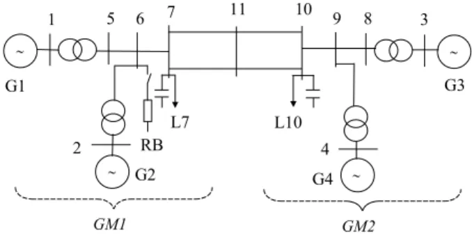
To illustrate capabilities of the proposed control this paper makes use of the four-machine power system, described in Fig. 1. Its characteristics are mainly inspired from [1]. For the simulations purpose all the generators are modeled as follows: detailed machine model with slow direct current exciter, automatic voltage regulator, and speed regulator. Other controls were not considered. The loads are modeled as constant current (active part) and constant impedance (reactive part). ∼ ∼ ∼ ∼ 5 1 6 7 8 3 4 2 9 11 10 G3 G4 G2 G1 RB L7 L10 GM1 GM2
Fig. 1 A four-machine power system
While the system operates in steady-state conditions, the generators G1, G2 (hydro) and G3, G4 (thermal) produce approximately the same active powers (700 MW) and the two loads L7, L10 consume respectively 990 and 1790 MW. The resistive brake (RB) is located at bus 6 and sized as g=5.0
p.u. mhos on a 100 MVA base (500 MW). This is a reasonable value in view of the fact that a 1400 MW braking resistor is presently in use [1,2].
A. State definition
We assume that the angle and speed of each generator are available (they can be either measured directly or estimated). The OMIB parameters are inferred using (10,11,12). GM1 is composed of machines G1 and G2 while GM2 is composed of machines G3 and G4. The state at time t is represented as,
) , ( t t t s = δ ω . (13) B. Reward definition
It is critical that the rewards truly indicate what is wanted to be accomplished, not how it is wanted to be achieved [13]. For the particular problem considered in this paper the aim of the RL controller is twofold: to improve damping of rotor angle
oscillations of all generating units in the system and to enlarge the stability domain. These oscillations are observable in the magnitudes of OMIB angle and speed, and the aim of the controller is to limit their magnitudes. The resistive brake should be switched on only when large oscillations occur. All this can be accomplished by defining the reward as,
= − ≠ − − − − = + + + + term 1 t term 1 t 1 t 2 eq 1 t 1 t s s if 1000 s s if u c c r δ δ ω , (14)
where is the OMIB post-fault equilibrium angle, u is the cost associated with the brake being on. The purpose of weighting factors c and is to bias the control efforts toward damping of the OMIB angle or the OMIB speed. The higher the cost , the less the controller will act on small perturbations. In order to deal with the loss of stability, a terminal state ( ) is introduced. This state is reached when the system has lost stability and a very bad value for the reward (-1000) is then obtained. We consider that the system has gone outside of the stability domain when .
eq δ 1 c2 u term s o t ≥180 δ C. The values of parameters
The measured (directly or indirectly) quantities are individual machines angle and speed. The period between two samplings is chosen equal to 50ms which means that the value of the control {0,1} could change every 50ms. A large value of γ implies the algorithm will take long-term benefit control actions. However, a too large value (a value close to 1) can lead to convergence problems. Simulations carried out have shown that γ=0.98 represents a reasonable tradeoff. The values of parameters in (14) are chosen as c1=0.0, c2=1.0, and
. These values indicate that the control efforts are fully biased toward control of the OMIB speed (to avoid difficulties associated with the estimation of post-fault equilibrium OMIB angle). ε-greedy factor is set to 0.1 which means that a random action will be taken at each 10-th sampling on average. The factor
0 2 u= .
ε is set to rather high value to encourage the RL algorithm exploration. The OMIB angle and speed are uniformly discretized in 100 values within the interval [-3.15,3.15] rad and [-10,10] rad/s, respectively.
D. Control law learned
The RL algorithm is used to learn the optimal closed-loop control law (strictly speaking, the closed-loop control law learned will be different from the optimal one due to the facts that the input signal of the RL algorithm is discretized and represents something else than the system real state). But to each power system configuration corresponds an optimal control law. The strategy proposed here is to realize the learning by using always the same configuration and to assess the control law robustness to justify the use of the control law in configurations that do not correspond to the one in which the learning has been done.
V. SIMULATION RESULTS
A. Scenario description
The learning period is partitioned into different scenarios. Each scenario starts with the power system being at rest and is such that at a short-circuit at bus 10 occurs. The fault duration is chosen at random in the interval
s 10
[
0,350ms]
. The scenario stops either when the instability is reached or whentis greater than . The only reason for realizing a short-circuit during a scenario is to drive the system far from the equilibrium point. Otherwise the learning would only happen in areas close to the equilibrium point. Because we do not want to learn the optimal closed-loop control law that corresponds to the fault-on configuration, we do not realize any learning during the fault period (the
four-uple is never used as input of the RL
algorithm if s 60 ) 1 + , ,rt st , (st ut
t and/or correspond to the fault
configuration time interval). The total number of scenarios equals to 1000, out of which 115 were unstable.
1 t+
B. Performance index
The learning performance (the quality of the control) is measured by introducing the discounted return at time t
∑
= − = tf t k k t k t r R γ , (15) where is equal either to , when terminal state (loss of stability) is not reached, or to the time when terminal state is reached. This measure indicates two things. The first one is the distance from the system equilibrium point at timef
t 60s
t (one can reasonably suppose that if at time t we are far from the equilibrium point, will be bad). The second one is the control quality. Indeed, if the quality of the control law is “good” one can expect while being in state
t
R
s at time t better
return Rt than if we were using a “bad” control law. C. Control law performances
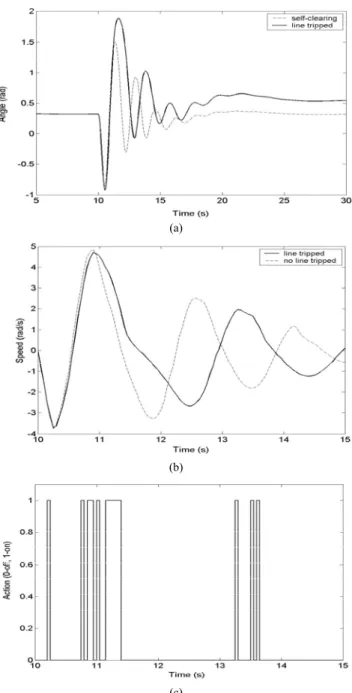
Evolutions of at different stages of the learning process are represented in Fig. 2. They all correspond to scenarios for which the fault duration is equal to . After the first 10 learning scenarios the value of is still rather low. The control law learned is far from the optimal one due to the rather small learning time. As the number of scenarios increases the quality of control is improving. As we can observe it, the value of converges to zero for the curves labeled “70 scenarios” and “100 scenarios”. It means that the system reaches its equilibrium point and that no control actions are taken when the system is at rest. Fig. 3 represents the evolution of the OMIB angle, speed, and actions taken after convergence of the learning process. To highlight the control benefit in terms of damping, the OMIB angle of the uncontrolled system is given in Fig. 3a, and corresponding OMIB speed in Fig. 3b.
t R ms 215 t R t R
The controller successfully learned to control efficiently the system using 7 brake switches. These curves have been drawn with ε-greedy factor set to 0 what in turn means that the controller uses only greedy actions to control the system.
Fig. 2 A zoom on learning performance evolution
(a)
(b)
(c)
Fig. 3 Evolution of the OMIB angle, speed, and control actions taken (215 ms duration self-clearing fault)
D. Control law robustness
To assess the robustness of the proposedcontrol, the learned control law is used to control the system when subjected to a different fault scenario. The system response and actions taken are illustrated in Fig. 4 together with the controlled system response to the self-clearing short-circuit. In spite of the change in system configuration, the controller succeeds to control efficiently the system being subjected to the “unseen” scenario. This is due to the high robustness of the closed-loop control law learned. Note that the uncontrolled system loses stability for this scenario.
(a)
(b)
(c)
Fig. 4 Evolution of the OMIB angle, speed, and control actions taken (215 ms duration fault cleared by opening the line 11-10)
E. Enlarging of the stability domain
For the duration self-clearing fault, the uncontrolled system loses stability after the fault clearance, but by using learned control law the controller stabilizes the system.
ms 350
s 75 1.
The evolution of the OMIB angle is illustrated in Fig. 5 for both controlled and uncontrolled system.
Fig. 5Evolution of the OMIB angle (350 ms duration self-clearing fault)
F. Remarks and discussion
The primary objective of the paper is to highlight the potential of RL application in controlling a dynamic brake aimed to enhance power system transient stability as well as the damping of large oscillations. Some practical limitations met when using the dynamic brake, such as the maximum insertion time and the maximum number of consecutive insertions, were not considered in the simulations. Maximum number of consecutive brake insertions can be handled by choosing proper switching costs. Further work is needed to adopt criteria for choosing proper switching costs to handle brake insertion constraints and accommodate different brake technological solutions. Proper use of the domain knowledge (the knowledge about the physical problem under consideration, that is the knowledge about power system dynamics) can resolve the curse of dimensionality problem and help RL methods to handle complex problems. This is particularly stressed in the paper by reducing the state-space dimensionality and defining the proper reward. Observe in Fig. 3,4, and 5 that the OMIB starts in a backswing (decelerating) mode. This is due to the fact that the short-circuit being located at the right part of the power system, group GM2 accelerates during the fault.
Although the control of particular system mode (inter-area oscillations) is considered in the paper the idea is much wider. Observe that the reward in (14) is defined in such a way that the control efforts can be biased toward slower as well as faster oscillations through proper choice of parameters and
. These parameters are introduced having in mind further extension of the control toward a multi-agent control system (a number of distributively located brakes controlled by individual agents) where a coordination agent can be placed upon local ones and learn appropriate coordination through the settings of the parameters. However, simulations performed revealed that one’s good choice is to set parameter to 0 and avoid angle estimation in the system post-fault equilibrium. This is not conclusive and further work is needed to find an appropriate estimation algorithm with the aim of strengthening approach flexibility. 1 c 2 c 1 c
An issue not considered in this paper is the inclusion of communication delays. The work is underway to tackle this issue along recent theoretical results on MDP with delays and asynchronous cost collection, presented in [21].
VI. RELATED WORK
A similar approach where a resistive brake has been considered to enhance overall dynamic performance of a power system rather than individual power plants was presented in [2]. A classical DP algorithm was used to determine open-loop control laws for a number of anticipated fault durations. Time-invariant OMIB was used to resolve curse of dimensionality problem. Each obtained solution was then stored in a look-up table for use in real-time. The approach presented in this paper generalizes over the methodology from [2] in several ways:
- It determines closed-loop control law,
- The fault durations are not anticipated but rather chosen at random within a pre-specified interval,
- It uses generalized (time-varying and more accurate) OMIB to resolve curse of dimensionality problem.
A variety of approaches were considered and implemented, to decide when to switch ON or OFF the resistor [6], [18], [19]. All the approaches were implemented with the main aim of improving dynamic performances of individual power plants (usually hydraulic) and it is hard to compare them with the approach advocated in this paper.
Fortunately, one of the attractions of RL approach is the flexibility this approach provides while designing controllers for a given problem. Different heuristics as well as domain specific knowledge can be easily injected into the RL agent. This can be done by proper reward definition (e.g., additional penalty can be added into reward if insertion time is longer than allowed) or by proper initialization of Q function.
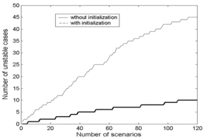
For illustration a simple heuristic [18] that the brake should be ON whenever and as long as the speed is positive is used to initialize Q function. Comparison of the learning process improvement is illustrated in Fig. 6 in terms of unstable cases met during the learning process in first 120 scenarios.
Fig. 7 Number of unstable cases with and without using heuristic to initialize
Q function
Observe that initialization of the Q function results in considerably smaller amount of the unstable cases and thus
increases the learning process reliability.
It is also possible to exploit in RL the information gathered by observing how an existing controller (e.g., one presented in [20]) acts and then to use RL to learn starting from that policy. The resulting policy should, in principle, outperform the original controller.
VII. CONCLUSIONS
The use of a resistive brake to enhance overall dynamic performance of the power system has been presented. A model based RL algorithm, known as prioritized sweeping, has been proposed to determine the approximation of the optimal switching strategies of the brake. The domain knowledge has been used to resolve the curse of dimensionality problem and to define the reward. Simulations were carried out on a synthetic four-machine power system. The results observed qualify the proposed control as effective to handle the problem considered. Although some practical limitations in the use of the resistive brake were not considered we suggest that RL based control, together with a proper use of the domain knowledge, offers attractive features for practical applications.
VIII. APPENDIX
GENERIC ALGORITHM FOR MODEL BASED LEARNING METHOD Initialize Q(s,u)= ,0 ∀s∈S and ∀u∈U
Initialize parameters of the model:
U u and S s s 0 u s s N(' , )= , ∀, '∈ ∀ ∈ U u and S s s 0 u s s p(' , )= , ∀, '∈ ∀ ∈ U u and S s 0 u s r( , )= , ∀ ∈ ∀ ∈ Do forever:
Observe current state s
Choose action u from s using knowledge of Q (e.g. ε−greedy) Take action u and observe s' and r .
Update model: S i u s i N u s s N(' , )←β ( , ), ∀∈ , ) , ( ) , ( ) , ( ) , (
∑
∑
∈ ∈ + + ← S j S j 1 u s j N r u s j N u s r u s r , ) , ' ( ) , ' (ssu N ssu 1 N ← + S i u s j N u s i N u s i p S j ∈ ∀ ←∑
∈ , ) , ( ) , ( ) , ( Compute Q by solving (9) ' s s←The ε -greedy method used to choose the action suggests that there is probability ε that the action chosen is not necessary the one which minimizes , but an action taken at random. This provides the algorithm with some exploratory behavior such that on average each
Q
ε /
1 time a random action is taken. The N function used in this algorithm does not intervene to describe the model as such but is necessary for its updating.
The term provides the algorithm with some
adaptive behavior by giving more importance (if ) (0≤ 1 β β ≤ 1 < β ) to the last data acquired.
IX. REFERENCES
[1] P. Kundur, Power System Stability and Control, McGraw Hill, 1994
[2] D. L. Lubkeman, G. T. Heydt, “The application of dynamic programming in a discrete supplementary control for transient stability enhancement of multimachine power system”, IEEE Trans. on PAS, Vol.
PAS-104, No. 9, pp. 2342-2348, Sept. 1985.
[3] M. Pavella, D. Ernst, D. Ruiz-Vega , Transient Stability of Power System
– A Unified Approach to Assessment and Control, KAP, 2000.
[4] E. De Tuglio, M. Dicorato, M. La Scala, P. Scarpellini, “A corrective control for angle and voltage stability enhancement on the transient time-scale”, IEEE Trans. on Power Systems, Vol. 15, No. 4, pp. 1345-1353, 2000.
[5] C. Taylor (convener), “Advanced angle stability controls”, CIGRE Technical Brochure. [Online]. Available:
http://www.transmission.bpa.gov/orgs/opi/CIGRE.
[6] CIGRE SC38-WG02, “State of the art in non classical means to improve power system stability, Electra, No. 118, pp. 87-113, May 1988. [7] C. Druet, D. Ernst, L. Wehenkel, “Application of reinforcement learning
to electrical power system closed-loop emergency control”, in Proc.
2000 PKDD2000, Lyon, France, pp. 86-95.
[8] B. H. Li, Q. H. Wu, “Learning coordinated fuzzy logic control of dynamic quadrature boosters in multimachine power systems”, IEE Part
C-Generation, Transmission, and Distribution, Vol. 146, No. 6, pp.
577-585, 1999.
[9] D. Ernst, L. Wehenkel, “FACTS devices controlled by means of reinforcement learning algorithms”, in Proc. 2002 14-th PSCC, Sevilla, Spain, Paper 18-6.
[10] H. You, V. Vittal, J. Jung, C. C. Liu, M. Amin, R. Adapa, “An intelligent adaptive load shedding scheme”, in Proc. 2002 14-th PSCC, Sevilla, Spain, Paper 17-6.
[11] T. P. Imthias Ahamed, P. S. Nagendra Rao, P. S. Sastry, “A reinforcement learning approach to automatic generation control”,
Electric Power Systems Research, vol. 63, pp. 9-26, Aug. 2002.
[12] A. W. Moore, C. G. Atkeson, “Prioritized sweeping: reinforcement learning with less data and less real time”, Machine Learning, vol. 13, pp. 103-130, 1993.
[13] R. S. Sutton, A. G. Barto, Reinforcement Learning: An Introduction, MIT Press, 1998.
[14] R. Bellman, Dynamic Programming, Princeton University Press, 1957. [15] D. P. Bertsekas, J. N. Tsitsiklis, Neuro-Dynamic Programming, Athena
Scientific, Belmont, MA, 1996
[16] C. G. Atkeson, J. C. Santamaria, “A Comparison of direct and model-based reinforcement learning”, International Conference on Robotics and Automation, 1997. [Online]. Available:
http://www.cc.gatech.edu/fac/Chris.Atkeson/publications.html
[17] Y. Xue, “A new method for transient stability assessment and preventive control of power system”, PhD Thesis, University of Liège, Belgium, 1988.
[18] S. S. Joshi, D. G. Tamaskar, “Augmentation of transient stability limit of a power system by automatic multiple application of dynamic braking”,
IEEE Trans. On PAS, Vol. PAS-104, No. 11, pp. 3004-3012, 1985.
[19] H. Jiang, D. T. Habelter, K. V. Eckroth, “A cost effective generator brake for improved generator transient response”, IEEE Trans. on Power
Syst., Vol. 9, No. 4, pp. 1840-1846, 1994.
[20] Y. Wang, W. Mittelstadt, D. J. Maratukulam, “Variable structure braking resistor control in a multimachine power system”, IEEE Trans. on Power
Syst., Vol. 9, No. 3, pp. 1557-1562, 1994.
[21] K. V. Katsikopoulos, S. E. Engelbrecht, “Markov Decision Process with delays and asynchronous cost collection”, IEEE Transactions on Automatic Control, Vol. 48, No. 4, pp. 568-574, 2003.