Enhanced performance for GPS-PPP by resolving bias-free
ambiguities
Thèse
Omid Kamali
Doctorat en sciences géomatiques
Philosophiæ Doctor (Ph.D.)
Québec, Canada
Enhanced performance for GPS-PPP by resolving
bias-free ambiguities
Thèse
Omid Kamali
Sous la direction de :
Marc Cocard, directeur de recherche
Rock Santerre, codirecteur de recherche
iii
Résumé
Le Positionnement Ponctuel Précis (PPP) est une technique de positionnement qui utilise un seul récepteur GNSS. Cette approche diffère nettement des méthodes différentielles qui sont largement utilisées et qui nécessitent deux ou plusieurs récepteurs. Le PPP est une technique économique, autonome par station, avec une précision centimétrique qui a ouvert la possibilité à une large gamme d'applications. Cependant, dans les applications qui nécessitent une convergence rapide et une haute précision, la performance du PPP n'est pas encore suffisante. Le PPP peut prendre jusqu’à 30 minutes pour converger vers des solutions avec une précision décimétrique. Cette longue période d’initiation est principalement consacrée à la stabilisation des ambiguïtés de phase vers des valeurs flottantes constantes. Compte tenu de ce problème, il est démontré que la Résolution des Ambigüités (RA) améliore la stabilité du modèle d’estimation, réduit le temps de convergence et améliore la précision des coordonnées. Cette étude vise donc à améliorer la performance du PPP pour obtenir une meilleure précision plus rapidement. À cette fin, les biais de phase des satellites qui perturbent la résolution des ambiguïtés sont estimées du côté producteur et résolues du côté utilisateur. Une modélisation judicieuse de paramètres et une sélection rigoureuse des modèles de correction sont effectuées afin de réduire la propagation des erreurs non-corrigées dans les biais de phase des satellites estimés.
Du côté producteur, une nouvelle approche modulaire à deux étapes est proposée et implémentée comprenant l'estimation de biais de phase des satellites à partir de chaque site et l'intégration séquentielle des solutions. Ces deux étapes ont des structures simples et elles permettent d'estimer précisément les biais de phase de chaque satellite. L’algorithme de l’intégration séquentielle garde un bon compromis entre la charge de calcul, la charge et la capacité de mémoire de l’ordinateur, l'efficacité du traitement des paramètres et la précision des estimations. Du coté producteur, chaque observation est modélisée individuellement et intégrée dans le processus d'estimation. Ceci facilite l'intégration des fréquences supplémentaires (par exemple, la troisième fréquence L5 ou des observations multi-GNSS) pour améliorer davantage la performance de PPP en fonction de la modernisation du GNSS.
Du côté utilisateur, un modèle d’observation de plein rang au niveau de récepteur mono-fréquence est proposé et implémenté. Cela donne de la flexibilité aux utilisateurs avec les récepteurs mono-fréquence pour utiliser notre solution PPP-RA lorsque les produits d'ionosphère de haute précision sont disponibles. Le modèle proposé est compatible avec les horloges de satellite standards actuelles fournies par IGS, CODE, JPL, par exemple. Le délai ionosphérique est corrigé et estimé en parallèle. Cela permet à l'utilisateur d’utiliser une correction ionosphérique de faible ou de haute précision et obtenir une performance améliorée en ajustant uniquement la précision de l'estimation de ce paramètre.
iv
La performance du PPP-RA du côté utilisateur a été comparée au PPP conventionnel en termes du temps de convergence et de la précision des coordonnées. En résumé, on a obtenu une amélioration importante en temps de convergence (jusqu'à 80 %) et en précision planimétrique (jusqu'à 60 %) par rapport au PPP conventionnel. De plus, une étude comparative est effectuée pour distinguer les caractéristiques de notre approche des autres méthodes PPP-RA. L’avantage de notre PPP-RA est aussi démontré par son approche unique à éliminer les défauts de rang et résoudre les ambiguïtés libre-de-biais.
v
Abstract
Precise Point Positioning (PPP) is a single receiver GNSS positioning technique developed in contrast to broadly used differential methods that require two or more receivers. Employing a single receiver makes PPP a cost-effective and per-site autonomous technique with centimetre precision that has opened up the possibility of a wide range of applications. In many applications where short time period is required to reach high precisions, the performance of PPP is not yet sufficient. Typically, PPP takes up to 30 minutes in order to converge to coordinate solutions with acceptable precision. This limitation is mostly due to the long period required for stabilizing the float carrier phase ambiguities to constant values. Given this problem, it is showed that Ambiguity Resolution (AR) improves drastically the stability of the estimation model that in turn reduces the convergence time, and increases the precision of estimated coordinates. Thus, this study seeks to enhance the performance of PPP to obtain higher precision at a faster convergence time. For this reason, the hardware dependent satellite phase biases are estimated at the producer-side and by applying them as corrections the integer ambiguities can be resolved at the user-side. A judicious modelling of all parameters and a careful selection of the correction models is accomplished to reduce the impact of error propagation on the precision of parameters estimation.
At the producer-side, a novel modular approach is proposed and established including the per-site satellite phase bias estimation and the sequential integration of the solutions. The two-steps of the producer-side have simple structures and allows for estimating the satellite phase biases. The proposed sequential network solution, keeps a good compromise between the computational burden, the computer memory load, the efficiency of handling parameters and the precision of estimations. In addition, all observables are modelled individually and integrated in the estimation process that facilitates the extension of algorithms for integrating additional frequencies or mutli-GNSS observables with respect to the GNSS modernization.
At the user side, a novel full rank design matrix in the single frequency level is proposed and implemented. This gives the flexibility to the users with single-frequency receivers to benefit from our PPP-AR while the high precision ionosphere products are available. The proposed model is compatible with the current standard satellite clocks available, for example, from IGS, CODE, and JPL. The ionosphere is corrected and estimated at the same time. This gives the user the possibility to take advantage of low or high precision ionosphere products for obtaining an enhanced performance with our PPP-AR by only adjusting the precision of the ionosphere delay estimation.
The performance of our PPP-AR user-side is then compared to the conventional PPP in terms of convergence time and coordinate precision. A substantial improvement has been obtained in terms of planimetric precision
vi
(up to 60%) and the convergence time (up to 80%) compared to the conventional PPP method. In addition, the characteristics of our PPP-AR are compared in detail with other PPP-AR methods. The advantage of our method is discussed by its unique approach of removing the rank deficiencies and resolving bias-free ambiguities.
vii
Table of Contents
Résumé ... iii
Abstract ... v
Table of Contents ... vii
List of Tables ... xi
List of Figures ... xiii
List of Symbols ... xvi
List of Acronyms ... xix
Acknowledgments ... xxii
Introduction ... 1
1.1 Motivation ... 1
1.2 Hypothesis and Objectives ... 2
1.3 Methodology ... 2
1.4 Contribution of this dissertation... 4
1.5 Dissertation outline ... 5 Literature review ... 7 2.1 Overview of GPS ... 7 2.2 Conventional PPP ... 9 2.2.1 Conceptual model ... 9 2.2.2 Receiver clock ... 10 2.2.3 Site displacement ... 11 2.2.4 Troposphere ... 12 2.2.5 Relativity ... 13 2.2.6 Satellite orbits ... 13 2.2.7 Satellite clock ... 14 2.2.8 Phase wind up ... 15 2.2.9 Code biases ... 16
2.2.10 Receiver and satellite antenna phase center ... 17
2.2.11 Cycle slip ... 18
2.2.12 Multipath ... 19
2.3 PPP-AR ... 19
viii
2.3.2 Ionosphere ... 20
2.3.3 Receiver and satellite phase biases ... 22
2.3.4 Review of PPP-AR methods ... 22
2.3.5 Interchangeability of PPP products ... 24
2.4 Integer ambiguity resolution ... 25
2.4.1 Integer ambiguity estimator ... 25
2.4.2 Integer ambiguity validation ... 28
2.4.3 Integer ambiguity transformations ... 31
2.4.4 Impact of unmodeled biases on ambiguity resolution ... 33
2.4.5 Partial Integer ambiguity resolution ... 33
2.4.6 Summarizing ambiguity resolution methods ... 35
2.5 PPP services ... 35
2.5.1 Online PPP ... 35
2.5.2 PPP software packages ... 37
2.5.3 Real-time PPP services ... 37
2.6 Integration of other systems... 39
2.6.1 Cooperative PPP ... 39
2.6.2 Multi-GNSS observables ... 40
2.6.3 RTK-PPP (SSR-RTK) ... 42
2.6.4 Other systems ... 43
2.7 Overview of our PPP-AR method ... 43
Setting up PPP-AR observation model and design matrix ... 45
3.1 Functional model ... 45
3.1.1 Observation models ... 45
3.1.2 Correction models ... 48
3.1.3 Categorizing parameters ... 53
3.2 Setting up partial design matrix for unknown parameters ... 53
3.2.1 Coordinates and site displacement partial design matrix ... 55
3.2.2 Receiver clock partial design matrices ... 55
3.2.3 Troposphere partial design matrix ... 56
3.2.4 Ionosphere partial design matrix ... 58
3.2.5 Receiver phase bias partial design matrix ... 60
ix
3.2.7 Satellite phase bias partial design matrix ... 61
3.3 Setting up complete PPP-AR design matrix ... 62
3.3.1 Producer-side design matrix ... 64
3.3.2 User-side design matrix ... 66
3.4 Estimation of PPP-AR parameters ... 67
3.4.1 Kalman filter adapted to random walk and pre-elimination ... 67
3.4.2 Partial integer ambiguity resolution method ... 70
Designing PPP-AR architecture and algorithms ... 71
4.1 Producer-side architecture ... 71
4.1.1 Module 1: per-site phase bias estimation ... 72
4.1.2 Module 2: sequential network solution ... 74
4.2 User-side architecture ... 79
4.3 Comparison with other PPP-AR methods ... 82
Producer-side experimental validations ... 89
5.1 Producer-side data set ... 89
5.2 Processing strategy ... 90
5.2.1 Per-site satellite phase bias estimation ... 90
5.2.2 Sequential network integration ... 91
5.3 WL satellite phase biases ... 92
5.3.1 Averaging WL phase bias... 95
5.4 L1 satellite phase biases ... 99
5.4.1 Averaging L1 phase biases ... 102
5.5 Phase biases validation ... 103
5.5.1 Validation network ... 103
5.5.2 Validation results ... 104
User-side experimental validations ... 111
6.1 User-side data set ... 111
6.2 Processing strategy ... 112
6.2.1 Blunder detection and removal ... 113
6.3 Performance of the ambiguity resolution ... 115
6.4 Performance in terms of coordinate precision ... 116
6.4.1 Coordinate solutions per-station: ... 116
x
6.4.3 Temporal improvement of precision ... 126
6.5 Performance in terms of convergence time ... 128
6.6 Comparison of AR impact on precision and convergence time ... 131
6.7 Comparison with other PPP-AR methods ... 132
Conclusions and future researches ... 137
7.1 Summary of results and analysis ... 137
7.2 Suggestions for future researches ... 141
References ... 145
Appendix A Anisotropic troposphere parameterization ... 159
Appendix B Computational aspects of data analysis ... 161
B.1 Computational load aspects ... 161
B.2 Imported external file formats ... 165
B.3 Computation hardware and operating system ... 166
B.4 Implementation specifications and features of results presentation ... 167
Appendix C Conventional PPP full rank design matrix ... 171
Appendix D Per satellite validation of the phase biases ... 173
Appendix E Satellite problems and maneuvers in year 2012 logged by CODE center ... 175
xi
List of Tables
TABLE 2.1OVERVIEW OF GPS CARRIER WAVES ... 8
TABLE 2.2OVERVIEW OF GPS DUAL-FREQUENCY COMBINATIONS AND THEIR BRIEF CHARACTERISTICS ... 9
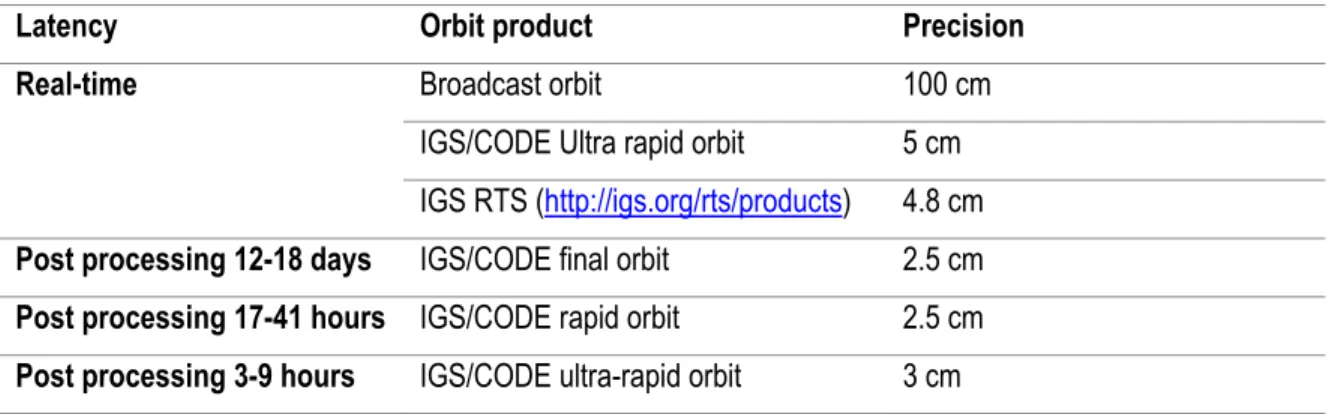
TABLE 2.3SUMMARY OF ORBIT PRODUCT PRECISION FOR REAL-TIME AND POST PROCESSING PPP APPLICATIONS .. 14
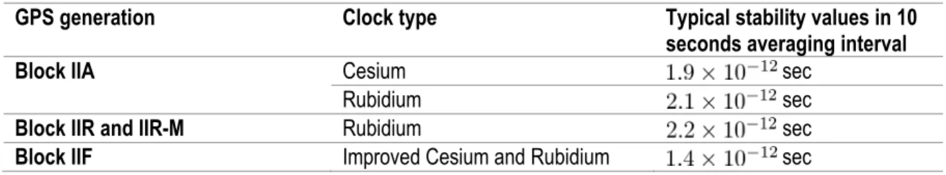
TABLE 2.4SUMMARY OF CLOCK PRODUCT PRECISION FOR REAL-TIME AND POST PROCESSING PPP APPLICATIONS . 14 TABLE 2.5GPS SATELLITES GENERATION CLOCK TYPES AND THEIR TYPICAL SHORT TERM STABILITY ... 15
TABLE 2.6SUMMARY OF GIM PRECISION FROM DIFFERENT PROVIDERS ... 21
TABLE 2.7SUMMARY OF ESTIMATOR CLASSES ... 26
TABLE 2.8SUMMARY OF THE CONVENTIONAL CLASS ESTIMATORS ... 26
TABLE 2.9POSSIBILITIES OF AMBIGUITY VALIDATION RESULTS ... 28
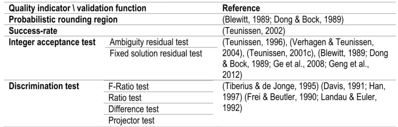
TABLE 2.10REVIEW OF THE CONVENTIONAL QUALITY INDICATORS OF THE INTEGER AMBIGUITIES ... 28
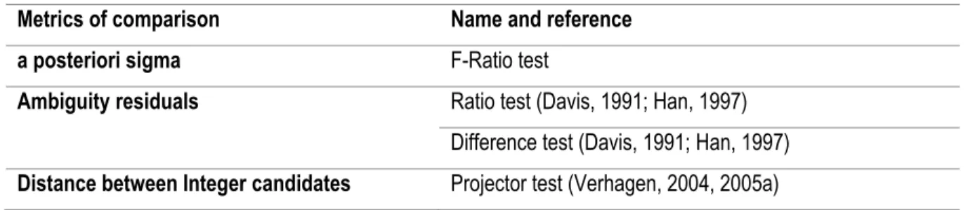
TABLE 2.11CONVENTIONAL DISCRIMINATION TESTS CATEGORIZED BY THEIR FUNDAMENTAL METRIC OF COMPARISON ... 30
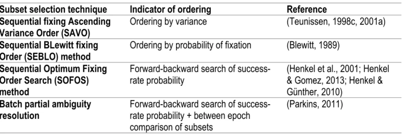
TABLE 2.12SUMMARY OF SUBSET SELECTION TECHNIQUES, THEIR INDICATOR OF ORDERING AND REFERENCE ... 34
TABLE 2.13SUMMARY OF THE CONVENTIONAL AMBIGUITY RESOLUTION METHODS (ARM) ... 35
TABLE 2.14SUMMARY OF SOME ONLINE PPP SERVICES ... 36
TABLE 2.15SUMMARY OF SOME PPP SOFTWARE PACKAGES ... 37
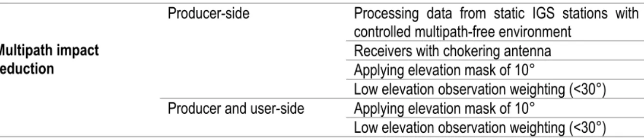
TABLE 3.1OUR COMBINED APPROACH FOR REDUCING AND MITIGATING MULTIPATH IMPACT ... 50
TABLE 3.2SUMMARY OF CORRECTION MODELS APPLIED IN THIS DISSERTATION ... 51
TABLE 3.3PARTIAL DESIGN MATRIX FOR CATEGORIZED PARAMETERS OF GPS OBSERVABLE MODEL ... 54
TABLE 3.4APPROACHES FOR REDUCING RANK DEFICIENCY IN GPS APPLICATIONS OBSERVATION MODELS ... 62
TABLE 3.5SUMMARY OF HANDLING UNKNOWN VARIABLES IN OUR PPP-AR MODEL AT THE PRODUCER-SIDE ... 64
TABLE 3.6SUMMARY OF HANDLING UNKNOWN VARIABLES IN OUR PPP-AR MODEL AT THE USER-SIDE ... 66
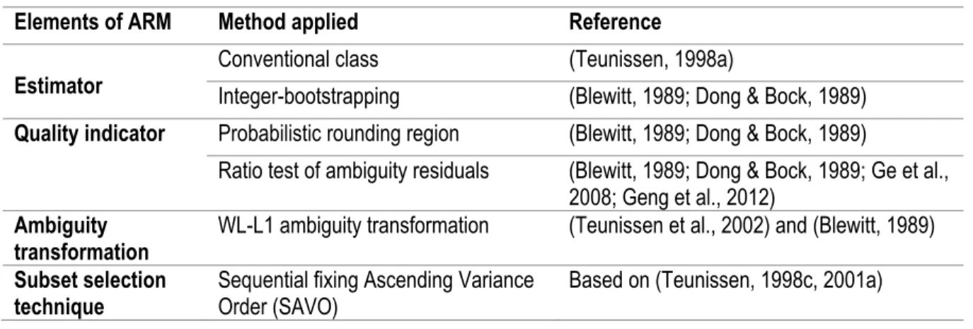
TABLE 3.7SUMMARIZING ELEMENTS OF OUR AMBIGUITY RESOLUTION METHOD (ARM) ... 70
TABLE 4.1DESCRIPTION OF THE MODULAR PARTIAL PHASE BIAS ESTIMATION AT THE PRODUCER-SIDE ... 71
TABLE 4.2SUMMARY AND COMPARISON BETWEEN OUR PPP-AR, CONVENTIONAL PPP AND OTHER PPP-AR METHODS IN THE CASE OF DUAL FREQUENCY OBSERVABLES WITH N OBSERVED SATELLITES IN A SINGLE EPOCH ... 83
TABLE 5.1SPECIFICATION OF THE PRODUCER-SIDE DATA SET ... 89
TABLE 5.2THE INITIAL PRECISION OF THE UNKNOWNS AT THE PRODUCER-SIDE ... 91
TABLE 5.3CONFIGURATION OF SEQUENTIAL NETWORK SOLUTION ... 91
TABLE 5.4RMSE OF AVERAGING THE WL PHASE BIASES WITH THE INTERVAL OF 24 HOURS DURING ONE YEAR (2012) SELECTED FOR THIS THESIS ... 95
TABLE 5.5DESCRIPTION OF THE PHASE BIAS VALIDATION ... 103
TABLE 5.6SPECIFICATION OF THE DATA SET USED FOR THE VALIDATION OF THE PHASE BIASES ... 103
TABLE 5.7PHASE BIAS VALIDATION RESULTS WITH 14 STATIONS FOR 32GPS SATELLITES IN YEAR 2012.*THE SESSIONS ARE PER SATELLITE AND PER DAY ... 104
TABLE 5.8STATISTICS ON THE IMPROVEMENT OF THE PRECISION OF THE WL AND L1 AMBIGUITY RESIDUALS AFTER APPLYING PHASE BIAS CORRECTIONS ON THE STATION NAIN,DOY10,2012. ... 108
TABLE 5.9STATISTICS ON THE PRECISION OF THE WL AND L1 AMBIGUITY RESIDUALS BEFORE AND AFTER APPLYING PHASE BIAS CORRECTIONS FOR ALL 32 SATELLITES IN YEAR 2012 OBTAINED FROM 14 VALIDATION NETWORK STATIONS ... 109
xii
TABLE 5.10F-RATIO TEST RESULTS OF THE WL AND L1 AMBIGUITY RESIDUALS BY APPLYING THE PHASE BIAS CORRECTION FOR ALL 32 SATELLITES FOR ONE YEAR (2012) ... 109
TABLE 6.1SPECIFICATION OF VALIDATION TEST DATA SET AND COMPUTATION OF USER-SIDE OF PPP-AR ... 112
TABLE 6.2INITIAL PRECISION OF THE UNKNOWNS AT THE USER-SIDE OF THE PPP-AR AND THE CONVENTIONAL PPP ... 113 TABLE 6.3SPECIFICATION OF THE CUSTOMIZED AMBIGUITY RESOLUTION METHOD ADOPTED IN THIS DISSERTATION
... 113 TABLE 6.4FAIL-RATE AND THE FIXED RATE AT THE USER-SIDE.(*THREE-HOUR SESSIONS) ... 114
TABLE 6.5SUMMARIZING THE TIME NEEDED IN WL AND L1 CASES FOR FIRST OCCURRENCE OF AMBIGUITY
RESOLUTION ORDERED BY SUCCESS-RATE PERCENTAGE ... 116
TABLE 6.6MEAN, MEDIAN AND STANDARD DEVIATION OF PRECISION IMPROVEMENT ... 127
TABLE 6.7CONVERGENCE TIME OF THE CONVENTIONAL AND THE PPP-AR FOR THE NORTH PRECISION FROM1 TO 10 CM IN RELATION TO THE AR SUCCESS-RATE ... 129
TABLE 6.8CONVERGENCE TIME OF THE CONVENTIONAL AND THE PPP-AR FOR THE EAST PRECISION FROM1 TO 10 CM IN RELATION TO THE AR SUCCESS-RATE ... 129
TABLE 6.9CONVERGENCE TIME OF THE CONVENTIONAL AND THE PPP-AR FOR THE ALTIMETRIC PRECISION FROM 3 TO 10 CM IN RELATION TO THE AR SUCCESS-RATE ... 130
TABLE 6.10CONVERGENCE TIME OF THE CONVENTIONAL AND THE PPP-AR FOR THE PLANIMETRIC PRECISION FROM1 TO 10 CM IN RELATION TO THE AR SUCCESS-RATE ... 130
TABLE 6.11COMPARISON OF PERFORMANCE (PRECISION AND CONVERGENCE TIME) OF OUR PPP-AR WITH OTHER
PPP-AR METHODS BASED ON LITERATURE RESULTS ... 133
TABLE B.1DESCRIPTION OF DATA LOAD USED FOR EXPERIMENTAL VALIDATION OF PROPOSED PPP-AR ... 165
TABLE B.2FORMATS SUPPORTED BY PPP-AR AND CONVENTIONAL PPP DEVELOPED IN THIS DISSERTATION ... 165
TABLE B.3SPECIFICATIONS OF CLUSTER COMPUTER APPLIED FOR PROCESSING DATA IN PPP-AR AND
CONVENTIONAL PPP SOFTWARE ... 166
TABLE B.4SPECIFICATIONS OF DESKTOP COMPUTER APPLIED FOR ANALYSING ALL PROCESSED DATA AND IN SECOND MODULE OF PRODUCER-SIDE FOR COMPUTING SEQUENTIAL NETWORK SOLUTION ... 166
TABLE B.5PROGRAMMING SPECIFICATIONS OF CONVENTIONAL PPP SOFTWARE, USER-SIDE PPP-AR SOFTWARE, AND FIRST MODULE OF PRODUCER-SIDE PPP-AR SOFTWARE ... 168
TABLE B.6PARALLEL SCRIPTING SPECIFICATIONS FOR INTEGRATING DEVELOPED SOFTWARE IN CLUSTER.SCRIPT APPLIED ON CONVENTIONAL PPP SOFTWARE, USER-SIDE PPP-AR SOFTWARE, AND FIRST MODULE OF
PRODUCER-SIDE PPP-AR SOFTWARE ... 168
TABLE B.7PROGRAMMING SPECIFICATIONS OF RESULT ANALYSIS AND SECOND MODULE OF PRODUCER-SIDE
PPP-AR SOFTWARE ... 169
TABLE D.8IMPROVEMENT RATE OF RMS,STD, AND KURTOSIS OF RESIDUAL AMBIGUITIES BY APPLYING PHASE BIAS CORRECTIONS (*SIGNIFICANT,**NOT-SIGNIFICANT) ... 173
xiii
List of Figures
FIGURE 2.1CONCEPTUAL MODEL OF CONVENTIONAL PPP ... 10
FIGURE 2.2CONCEPTUAL MODEL OF PPP-AR SEGMENTS ... 20
FIGURE 3.1RECURSIVE KALMAN-FILTER PROCEDURE AS ESTIMATOR OF PARAMETERS ... 69
FIGURE 4.1FLOWCHART OF THE PER-SITE PHASE BIAS ESTIMATION (MODULE 1) ... 73
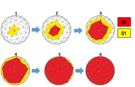
FIGURE 4.2OVERVIEW OF PROCESS OF ORDERING STATIONS FOR SEQUENTIAL CONTRIBUTION TO NETWORK SOLUTION ... 75
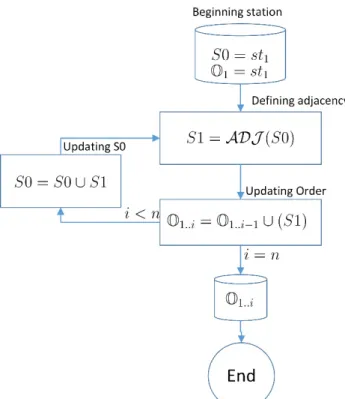
FIGURE 4.3DEFINITION OF THE ORDER OF THE SEQUENTIAL NETWORK SOLUTION BASED ON THE ADJACENCY OF THE STATIONS ... 76
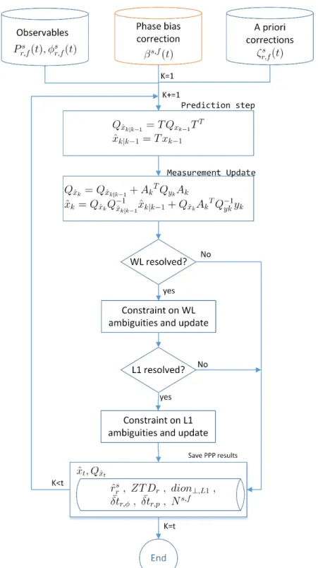
FIGURE 4.4FLOWCHART OF THE SEQUENTIAL NETWORK SOLUTION FOR THE ESTIMATION OF SATELLITE PHASE BIAS (MODULE 2) ... 78
FIGURE 4.5FLOWCHART OF THE USER-SIDE OF THE PPP-AR WITH THE INTEGER AMBIGUITY RESOLUTION ... 81
FIGURE 5.1PRODUCER-SIDE NETWORK (PSN) WITH 60 GLOBAL IGS STATIONS APPLIED FOR ESTIMATING THE SATELLITE PHASE BIASES ... 90
FIGURE 5.2INTERRELATED ADJACENT SITES OF PRODUCER-SIDE NETWORK (PSN) FOR ESTIMATING THE FINAL NETWORK SOLUTION OF WL AND L1 PHASE BIASES. ... 92
FIGURE 5.3WL PHASE BIASES FOR ALL GPS SATELLITES AND THEIR PRECISIONS IN DOY12 OF YEAR 2012 ... 94
FIGURE 5.4PROBABILITY DENSITY FUNCTION OF RESIDUALS [CYCLE] OF AVERAGING WL SATELLITE PHASE BIAS (CMP MODEL) IN 24 HOURS DURING ONE YEAR (2012).THE WIDTH OF THE BINS IS 1MM... 95
FIGURE 5.5THE RMS ERROR [CYCLE] OF AVERAGING THE WL PHASE BIASES IN THE INTERVAL OF 1,3…,360[DAYS] (X-AXIS).RESULTS FROM ONE YEAR (2012) PHASE BIASES ... 96
FIGURE 5.6ONE YEAR (2012) VARIATIONS OF THE WL SATELLITE PHASE BIASES [CYCLE] FOR EACH GPS SATELLITE ... 98
FIGURE 5.7GPS SATELLITE PRN24WL DAILY AVERAGED JUMPS CORRELATED WITH ERRORS DETECTED BY CODE CENTER ... 99
FIGURE 5.8(CONTINUED)L1 PHASE BIASES FOR ALL GPS SATELLITES AND THEIR PRECISIONS IN DOY12 OF YEAR 2012 ... 101
FIGURE 5.9RMS ERROR [CYCLE] OF AVERAGING THE WL(BLUE) AND THE L1(RED) PHASE BIASES FOR DIFFERENT INTERVAL [MIN](X-AXIS).RESULTS FROM ONE YEAR (2012) PHASE BIASES. ... 102
FIGURE 5.10RMS ERROR [CYCLE] OF AVERAGING THE WL(BLUE) AND THE L1(RED) PHASE BIASES FOR DIFFERENT INTERVAL [HOUR](X-AXIS).RESULTS FROM ONE YEAR (2012) PHASE BIASES. ... 102
FIGURE 5.11PHASE BIAS VALIDATION NETWORK WITH 14 GLOBAL IGS STATIONS ... 104
FIGURE 5.12DISTRIBUTION OF WL AMBIGUITY RESIDUALS [CYCLE] FOR STATION NAIN BEFORE APPLYING PHASE BIAS CORRECTIONS IN DOY10,2012(TOP).THE PROBABILITY DENSITY FUNCTION (PDF) OF AMBIGUITY RESIDUALS WITH THE INTERVALS OF 0.001[CYCLE](BOTTOM) ... 106
FIGURE 5.13DISTRIBUTION OF WL AMBIGUITY RESIDUALS [CYCLE] FOR STATION NAIN AFTER APPLYING PHASE BIAS CORRECTIONS IN DOY10,2012(TOP).THE PROBABILITY DENSITY FUNCTION (PDF) OF AMBIGUITY RESIDUALS WITH THE INTERVALS OF 0.001[CYCLE](BOTTOM) ... 106
FIGURE 5.14DISTRIBUTION OF L1 AMBIGUITY RESIDUALS [CYCLE] FOR STATION NAIN BEFORE APPLYING PHASE BIAS CORRECTIONS IN DOY10,2012(TOP).THE PROBABILITY DENSITY FUNCTION (PDF) OF AMBIGUITY RESIDUALS WITH THE INTERVALS OF 0.001[CYCLE](BOTTOM) ... 107
xiv
FIGURE 5.15DISTRIBUTION OF L1 AMBIGUITY RESIDUALS [CYCLE] FOR STATION NAIN AFTER APPLYING PHASE BIAS CORRECTIONS IN DOY10,2012(TOP).THE PROBABILITY DENSITY FUNCTION (PDF) OF AMBIGUITY RESIDUALS WITH THE INTERVALS OF 0.001[CYCLE](BOTTOM) ... 107
FIGURE 5.16PROBABILITY DENSITY FUNCTION (PDF) OF THE WL AMBIGUITY RESIDUAL WITH THE INTERVALS OF
0.001[CYCLE] BEFORE AND AFTER APPLYING PHASE BIAS CORRECTIONS OBTAINED FORM 14 VALIDATION NETWORK STATIONS FOR ALL 32 SATELLITES IN ONE YEAR 2012. ... 108
FIGURE 5.17PROBABILITY DENSITY FUNCTION (PDF) OF THE L1 AMBIGUITY RESIDUAL WITH THE INTERVALS OF
0.001[CYCLE] BEFORE AND AFTER APPLYING PHASE BIAS CORRECTIONS OBTAINED FORM 14 VALIDATION NETWORK STATIONS FOR ALL 32 SATELLITES IN ONE YEAR 2012. ... 108
FIGURE 6.1USER-SIDE NETWORK (USN) WITH 14 GLOBAL IGS STATIONS FOR THE ASSESSMENT OF THE USER-SIDE OF THE PPP-AR AND THE CONVENTIONAL PPP ... 112
FIGURE 6.2MEAN (BLUE) AND MEDIAN (RED) OF THE WL AMBIGUITY FIXED-RATE IN ONE YEAR (2012).THE THREE -HOUR SESSIONS (TOP) AND THE ZOOM ON THE FIRST 30 MINUTES (BOTTOM). ... 115
FIGURE 6.3MEAN (BLUE) AND MEDIAN (RED) OF THE L1 AMBIGUITY FIXED-RATE IN ONE YEAR (2012).THE THREE -HOUR SESSIONS (TOP) AND THE ZOOM ON THE FIRST 30 MINUTES (BOTTOM). ... 115
FIGURE 6.4NORTH COORDINATE COMPONENT OF THE CONVENTIONAL PPP(TOP) AND THE PPP-AR(BOTTOM) IN REFERENCE TO THE FINAL IGS RESULTS [METER] IN THREE-HOUR SESSIONS [HOUR] FOR USER-SIDE STATIONS IN YEAR 2012 ... 117
FIGURE 6.5EAST COORDINATE COMPONENT OF THE CONVENTIONAL PPP(TOP) AND THE PPP-AR(BOTTOM) IN REFERENCE TO THE FINAL IGS RESULTS [METER] IN THREE-HOUR SESSIONS [HOUR] FOR USER-SIDE STATIONS IN YEAR 2012 ... 118
FIGURE 6.6ALTIMETRIC COORDINATE COMPONENT OF THE CONVENTIONAL PPP(TOP) AND THE PPP-AR(BOTTOM) IN REFERENCE TO THE FINAL IGS RESULTS [METER] IN THREE-HOUR SESSIONS [HOUR] FOR USER-SIDE
STATIONS IN YEAR 2012 ... 119
FIGURE 6.7PLANIMETRIC COORDINATE COMPONENT OF THE CONVENTIONAL PPP(TOP) AND THE PPP-AR(BOTTOM) IN REFERENCE TO THE FINAL IGS RESULTS [METER] IN THREE-HOUR SESSIONS [HOUR] FOR USER-SIDE
STATIONS IN 2012 ... 120
FIGURE 6.8DAILY DISTRIBUTION OF THE USER-SIDE THREE-HOURS NORTH SOLUTIONS IN [METER] FOR THE
CONVENTIONAL PPP(TOP) AND THE PPP-AR(BOTTOM) IN REFERENCE TO THE IGS WEEKLY SOLUTION ... 121
FIGURE 6.9DAILY DISTRIBUTION OF THE USER-SIDE THREE-HOURS EAST SOLUTIONS IN [METER] FOR THE
CONVENTIONAL PPP(TOP) AND THE PPP-AR(BOTTOM) IN REFERENCE TO THE IGS WEEKLY SOLUTION ... 121
FIGURE 6.10DAILY DISTRIBUTION OF THE USER-SIDE THREE-HOURS ALTIMETRIC SOLUTIONS IN [METER] FOR THE CONVENTIONAL PPP(TOP) AND THE PPP-AR(BOTTOM) IN REFERENCE TO THE IGS WEEKLY SOLUTION ... 122
FIGURE 6.11DAILY DISTRIBUTION OF THE USER-SIDE THREE-HOUR PLANIMETRIC SOLUTIONS IN [METER] FOR THE CONVENTIONAL PPP(TOP) AND THE PPP-AR(BOTTOM) IN REFERENCE TO THE IGS WEEKLY SOLUTION ... 122
FIGURE 6.12PRECISION OF THE NORTH (TOP), AND EAST (BOTTOM) IN [METER] IN THE COURSE OF TIME [HOUR] AND IN REFERENCE TO THE IGS FINAL SOLUTIONS [METER] FOR THE PPP-AR(RED), AND THE CONVENTIONAL PPP
(BLUE) ... 123
FIGURE 6.13PLANIMETRIC (TOP), AND ALTIMETRIC (BOTTOM) PRECISION [METER] IN THE COURSE OF TIME [HOUR]
AND IN REFERENCE TO THE IGS FINAL SOLUTIONS [METER] FOR THE PPP-AR(RED), AND THE CONVENTIONAL
PPP(BLUE) ... 124
FIGURE 6.14PRECISION (RMS) OF NORTH COMPONENT IN [METER] FOR ALL THREE-HOUR SEGMENTS DURING 24 HOURS (GMT).THE CONVENTIONAL PPP(BLUE) AND THE PPP-AR(RED) IN YEAR 2012. ... 124
xv
FIGURE 6.15PRECISION (RMS) OF EAST COMPONENT IN [METER] FOR ALL THREE-HOUR SEGMENTS DURING 24 HOURS (GMT).THE CONVENTIONAL PPP(BLUE) AND THE PPP-AR(RED) IN 2012. ... 125
FIGURE 6.16PLANIMETRIC PRECISION (RMS) IN [METER] FOR ALL THREE-HOUR SEGMENTS DURING 24 HOURS
(GMT).THE CONVENTIONAL PPP(BLUE) AND THE PPP-AR(RED) IN 2012. ... 125
FIGURE 6.17ALTIMETRIC PRECISION (RMS) IN [METER] FOR ALL THREE-HOUR SEGMENTS DURING 24 HOURS (GMT).
THE CONVENTIONAL PPP(BLUE) AND THE PPP-AR(RED) IN 2012. ... 126
FIGURE 6.18PRECISION IMPROVEMENT RATE (%)(Y-AXIS) IN THE COURSE OF TIME (X-AXIS) FOR THE NORTH, EAST, UP AND PLANIMETRIC COMPONENT ... 127
FIGURE 6.19IMPROVEMENT RATE (%)(Y-AXIS) OF THE CONVERGENCE TIME WITH DIFFERENT LEVELS OF PRECISION
(X-AXIS) AND FOR THE NORTH, EAST, UP AND PLANIMETRIC COMPONENTS. ... 128
FIGURE 6.20SUCCESS-RATE OF L1(MEAN (BLUE) AND MEDIAN (RED)) DURING YEAR (2012) FOR THE USER-SIDE.IN THE HIGHLIGHTED PERIOD THE MEDIAN OF THE L1AR SUCCESS-RATE VARIES FROM 0% TO 100% ... 131
FIGURE 6.21COMPARISON OF THE IMPROVEMENT OF THE CONVERGENCE TIME AND THE PRECISION (%) BY AR
xvi
List of Symbols
Partial derivative
Between-satellite single difference Between-receiver single difference
Mean weighting function
Complimentary error function
. |. Conditional state
Norm Design matrix for code linear model Design matrix for phase linear model
Ambiguity Resolution Method
Adjacency Function Receiver phase bias [cycle] Satellite phase bias [cycle]
Temporal batch matrix with n batch of epochs
Lumped satellite phase bias
Bias propagated in ambiguities
Weighted mean value of epoch wise phase bias values k-th site satellite phase bias
Predicted satellite phase bias values for k-th site based on k-1th network solution Light speed in vacuum (299 792 458 m/s)
Constraint of rank for removing rank deficiencies User defined critical-value
Satellite differential code bias [meter] Receiver differential code bias [meter]
D Diagonal matrix in Cholesky decomposition
Dispersion Degree of freedom
Earth tide effect on the receiver position [meter] Code measurement noise + unmodeled errors [meter]
Phase measurement noise + unmodeled errors [meter] Residuals
First moment Index of frequency
Phase measurement [cycle] Frequencies
Integer mapping function in ambiguity resolution context
Normal distribution function
Height of ionosphere single layer above Earth’s surface [meter]
Ionosphere delay [meter]
Identity matrix of dimension (Matlab eye(n) command) Vertical ionosphere delay of frequencies
Elements of transformation matrix
xvii
Slant troposphere delay [meter]
Hydrostatic slant tropospheric delay [meter] Wet slant tropospheric delay [meter]
Index for predicting and updating steps in Kalman-Filter Wavelength of frequency f [meter]
Latitude, longitude of ionospheric piercing point L Lower triangular matrix of Cholesky decomposition
Multipath [meter]
Hydrostatic mapping function [-] Wet mapping function [-] Ionosphere mapping function [-] Integer phase ambiguity [cycle] Partial number of ambiguities
Estimated float ambiguities
, Number of observables
Number of unknown parameters Number of integer ambiguity parameters
Ocean loading effect on the receiver position [meter] Orbit determination error [meter]
Order of contribution of stations in sequential network solution Code measurement [meter]
Satellite Phase Center Offset [meter] Satellite Phase Center Variations [meter] Receiver Phase Center Offset [meter] Receiver Phase Center Variations [meter] Phase wind-up [cycle]
PDF over the pull in region
k-th site satellite phase bias covariance matrix
Predicted phase bias covariance matrix for k-th site based on k-1th solution Variance matrix of random walk process
Variance matrix of unknowns. Variance matrix of observables Index of receiver
Geometric distance between receiver and satellite [meter]
Relativity delay [meter]
Approximate value receiver coordinates Approximate value of satellite coordinates
Computed value of receiver coordinates Computed value of satellite coordinates
Increment of the receiver position Increment of satellite position Number of receivers
Random walk stochastic process Radius of the (spherical) Earth [meter] Index of satellite
xviii Number of satellites
Sparse matrix
S1 First degree adjacent stations in network solution
S0 Stations participated in network solution of satellite phase bias Pull-in-region
Variance of the weighted mean value of epoch wise phase biases ( ) Measurement time in GPS time [second]
TOF or Time Of Fly of GPS signal [second]
Offset of receiver clock
Offset of satellite clock
Receiver code clock [second]
Satellite code clock [second] Receiver phase clock [second] Satellite phase clock [second] Number of epoch or time batches
Duration of stacking for each batch parameter
Lumped receiver phase clock
Translation matrix in sequential Kalman filter solution
Transformation matrix for mapping observables to ionosphere-free Transition model matrix
Lumped satellite phase clock
Coefficient value matrix Estimated unknowns
Unknown parameters
Observables in least square solutions Hydrostatic Zenithal Total Delay [meter] Wet Zenithal Total Delay [meter] Zenith angle at receiver location [rad]
Zenith angle at ionosphere piercing point [rad] Correction models applied in observable models i-th arbitrary integer value (contextual parameter) Float ambiguity transformed by decorrelation matrix
xix
List of Acronyms
Aeronautical Radio Navigation Services (ARNS) Ambiguity Dilution Of Precision (ADOP)
Ambiguity Resolution (AR)
Ambiguity Resolution Method (ARM) Analysis Center Coordinator (IGS ACC) Automatic Precise Positioning Service (APPS) Best Linear Unbiased EStimator (BLUES)
Canadian Spatial Reference System PPP (CSRS PPP) Cascade Integer Resolution (CIR)
Center for Orbit Determination in Europe (CODE) Center of mass of the Earth system (CM) Center of mass of the solid Earth (CE) Coarse/Acquisition (C/A)
Collecte Localisation Satellites (CLS)
Centre National d’Études Spatiales, Toulouse, France (CNES) Differential Code Biases (DCB)
Double-Difference (DD)
Earth Orientation Parameter (EOP) Earth Rotation Parameter (ERP) Empirical orthogonal functions (EOF)
European Geostationary Navigation Overlay Service (EGNOS) European Space Agency’s Space Operations Centre (ESA/ESOC) European Union (E.U.)
FARA (Fast Ambiguity Resolution Approach) FASF (Fast Ambiguity Search Filter) Finite Element Solution 2004 (FES2004) Fractional Cycle Bias (FCB)
French Tidal Group (FTG) Geostationary Earth Orbit (GEO)
German Federal Agency for Cartography and Geodesy (BKG) Global Assimilative Ionospheric Model (GAIM)
xx Global Navigations Satellite Systems (GNSS)
GPS Analysis and Positioning Software (GAPS) IGS Analysis Centers (AC)
IGS ultra-rapid predicted (IGU-P) Inclined GeoSynchronous Orbit (IGSO) Integer Equivariant (IE)
Integer Least Square (ILS) International GNSS Service (IGS)
IONosphere MONitoring Facility (IONMON)
Japanese Multi-Functional Transport Satellite (MSAT) Jet Propulsion Laboratory (JPL)
L1 Civilian (L1C) L2 Civilian (L2C)
Least square AMBiguity Decorrelation Adjustment (LAMBDA) Least-Squares Ambiguity Search Technique (LSAST) Lumped AMBiguity PPP-AR (LAMB A PPP)
LUmped Satellite phase Clock PPP-AR (LUSC A PPP) Massachusetts Institute of Technology (MIT)
Medium Earth orbit (MEO) Military code (M)
Multivariate adaptive regression splines algorithm (MARS) Narrowlane (NL)
Natural Resources Canada (NRCan)
Optimal Method for Estimating GPS Ambiguities (OMEGA) Phase Center Offset (PCO)
Phase Center Variations (PCV) Precise Point Positioning (PPP) Probability Density Function (PDF)
Radio Technical Commission for Maritime Services (RTCM) Real-time GIPSY (RTG)
Real-time Precise Point Positioning (RT PPP) Real-time service (RTS)
REal-Time Clock Estimation system (RETICLE) Real-time Pilot Project (RTPP)
xxi Right Hand Circularly Polarized (RHCP)
Safety-of-Life (SoL)
Scripps Orbit and Permanent Array Center (SOPAC)
Semi-parametric multivariate adaptive regression B-splines (SP-BMARS) Sequential BLewitt fixing Order (SEBLO) method
Sequential fixing Ascending Variance Order (SAVO) method Sequential Optimum Fixing Order Search (SOFOS) method Solar radiation pressure (SRP)
Three Carrier Ambiguity Resolution (TCAR) Terrestrial Reference Frame (TRF)
Time Of Fly or (TOF) Total Group Delay (TGD)
Trimble Real-time eXtended (RTX) Ultraviolet limb scans (UVlimb) Un-calibrated Phase Delays (UPD) Universal Time (UT1)
University of New Brunswick (UNB) Universitat Politecnicia Catalunya (UPC) Vertical Total Electron Content (VTEC) Vienna Mapping Function 1 (VMF1) Wide Area Augmentation System (WAAS) Wide Area Differential GPS (WADPGS) Widelane (WL)
Widelane and phase bias (WLPB) Widelane satellite bias (WSB)
xxii
Acknowledgments
A long part-time project required help, motivation, and invaluable support of many people around me.
I would like, before all else, to sincerely acknowledge my supervisor professor Marc Cocard for inspiring me with his extensive scientific knowledge, his meticulous analytical reasoning. I personally believe that the PhD is a chance for acquiring the intellectual maturity that allows to profess a Philosophiae. This implies the possession of knowledge to apply to any given circumstance (personal, professional and scientific) for finding the answers with an optimum judgement and the optimal course of action. Attaining this understanding is not easy nowadays in most of research centers that focus merely on technical output. Marc, gave me the freedom and lots of independence to build a self-estimated satisfying scientific vision in one of the most challenging subjects of satellite geodesy. It has been a complex endeavour and I am absolutely grateful for the end result. I would like to deeply thank my co-supervisor professor Rock Santerre for whom I have great respect. Rock helped me structure, make concert progress, and improve substantially the quality of my work. His highly organized and pragmatic approach in supervising and his countless experience in Geodesy scientific works helped me to create a frame for finalizing and enhancing my work. A special thanks goes to Stéphanie Bourgon for her friendly discussions, advices and helps in my work.
Several organizations have contributed in financing my research: the GEOIDE (GEOmatics for Informed DEcisions) Network phase III, the Natural Sciences and Engineering Research Council of Canada (NSERC) attributed to Rock Santerre, Fond de soutien de Faculté de Foresterie, de Géographie et de Géomatique (FFGG). All these supports are gratefully acknowledged. I would like to thank CRG (Centre de Recherche en Géomatique) and REGARD laboratory for the access to the cluster computer for processing data.
Last, but not least, I need to appreciate the constant support of my family and my friends. Special thanks to Sebastian Meghezi, Daniel Macias for their friendly conversations during this long journey. I would like to dedicate this thesis to my parents and to my best friend Soudeh, thanking them for their endless support.
1
Introduction
1.1 Motivation
The conventional Precise Point Positioning (PPP) (Zumberge et al., 1997) has become a popular technique that uses a single receiver to reach centimetric precision. The precise point positioning, requires less infrastructure compared to the classical relative positioning methods. It makes PPP a more cost-effective approach. PPP has shown the potential of broad range of applications such as precise positioning in the isolated or rural areas with no available reference stations, the marine applications, the civil aviation, the agriculture industry, the seismic monitoring, the deformation monitoring (Bisnath & Gao, 2007; Zheng et al., 2014) and the geophysical studies. Many benefits of PPP such as the high precision positioning, the per-site autonomy with the continuous operation, and the cost-effectiveness have opened its potential to varied applications that attracted the attention of the commercial sector.
PPP takes up to 60 minutes in order to converge solutions to 5 cm (Seepersad & Bisnath, 2014a), stabilize the float carrier phase ambiguities to constant values, and achieve its optimal precision. In the applications where the fast initial convergence or re-convergence of the high precision positioning is necessary, PPP solution is not sufficient. In order to overcome this problem of the long convergence time and improve the precision of PPP, different factors can be considered. For instance, improving the quality of the observables, improving the predictability of the dynamic of the receiver, providing an external information about the receiver’s environment, improving the predictability of the receiver clock, improving the precision of the a priori correction models, and improving the redundancy by integrating other navigation systems observables. The common point between all these factors is their impact on the stability and the robustness of the estimation model to improve the performance of PPP.
Fixing the ambiguities improves drastically the stability of the estimation model that in turn reduces the convergence time and improves the precision of the estimated coordinates (Seepersad & Bisnath, 2014b). This is in contrast with the conventional PPP where no ambiguity resolution is integrated and simply all the float ambiguities are stacked (Héroux et al., 2001; Héroux & Kouba, 2001). The method of improving the performance of PPP with the ambiguity resolution has the flexibility to be combined with other improvement methods such as the multi-GNSS or INS integration.
Our main motivation is therefore, improving the performance of PPP by the ambiguity resolution. In addition, we seek to give the user, the flexibility to obtain improved performance even with a single-frequency receiver while the high precision ionosphere products are available.
2
1.2 Hypothesis and Objectives
The main hypothesis of this dissertation is that at the producer-side, the satellite phase biases can be estimated with low computational burden algorithms, usable for low capacity computers, and at the user-side, the performance of PPP can be improved by fixing integer ambiguities. The improvement implies a shorter convergence time and a more precise positioning result. PPP research community has come to the consensus of considering two indicators for the performance of PPP including the initial convergence time and the precision of positioning (Bisnath & Gao, 2007). The general objective is improving these two indicators of the performance of PPP by the integer ambiguity resolution. This general objective will be implied in the context of the post processing static stations with the following specific objectives:
The first specific objective is mitigating the fractional-cycle biases from the integer ambiguities. The hardware dependent phase biases originate from the transmitter and the receiver with the values of the fractional part of a cycle (Blewitt, 1989). These biases prevent integer ambiguity resolution because of their fractional nature.
The second specific objective is keeping the functional model full rank in the single-frequency level. By reaching this objective, PPP users with the single-frequency receiver are enabled to obtain the improved performance with the ambiguity resolution while the high precision ionosphere products are available.
The third specific objective is combining the merits of Ambiguity Resolution (AR) and the current official and widely accessible Ionosphere Models (IM). This is in the view of advancing the concept of PPP with the ambiguity resolution to take advantage of the available high or low precision ionosphere models. This specific objective considers mainly the accessibility of the global ionosphere models (GIM) and the growing availability of the high precision regional ionosphere corrections.
The fourth specific objective of this dissertation is developing a PPP-AR that is compatible with the current official and the widely accessible precise products (such as the IGS or CODE precise clocks, etc.). This is in view of profiting from the current state of the precise products for improving the performance of PPP.
1.3 Methodology
In order to resolve the integer ambiguities, the partial phase bias must be separated from the real-valued ambiguities. For this reason, we propose a PPP-AR model with two segments the producer-side and the side. In this PPP-AR model, the phase biases are estimated at the producer-side and provided to the
user-3
side. This will empower the user-side to obtain the improved PPP performance by resolving the integer ambiguities. Our PPP-AR has been implemented in two stages. The first stage includes designing the mathematical model, optimizing, integrating, and programming the software. The second stage includes validating the improvements, and the algorithms by processing real GPS data. The following steps can be summarized at the producer-side and the user-side.
The producer-side:
In the first step, the satellite phase biases are estimated independently for each reference site of the tracking network. The coordinates of the reference sites are fixed to their best-known values. The receiver phase bias is estimated as a part of the receiver phase clock. The satellite phase biases are lumped with the integer ambiguities at the producer-side. They can then be separated from the integer ambiguities as the fractional part of a cycle. This step is called the per-site phase bias estimation.
In the second step, the per-site solutions of the satellite phase biases are combined to obtain the precise network solutions and a continuous daily time series of the phase biases. In order to combine the estimations of the satellite phase bias, a sequential network solution is proposed. Processing the sequential network solution reduces drastically the computational burden and the memory load by limiting the set of parameters required to be present in the computer memory. It also improves the simplicity of handling the parameters, the computing algorithms, and the debugging process.
At the end, a quality control process is developed for validating the satellite phase biases before delivering them to the user-side. This test is designed to accept/reject the daily time series of the Wide-Lane (WL) and the L1 satellite phase bias. The rejected phase biases are flagged, and the users can down weight or exclude their corrections.
The user-side:
The user-side PPP algorithms integrate the partial phase biases provided by the producer-side in order to resolve ambiguities. At the user-side, the following characteristics can be distinguished from the producer-side process.
All coordinates are unknown and estimated. The partial phase biases estimated at the producer-side are applied as the correction to the phase measurements. The wide-lane (WL) ambiguities are fixed in the parameter domain. Fixing the WL ambiguities stabilizes the narrowlane (NL/L1) ambiguities. the narrowlane (NL/L1) ambiguities can then be promptly fixed to the integer values (Blewitt, 1989).
4
The design matrix is set-up full rank in the single-frequency level. This gives the user the flexibility to obtain the improved performance even with a single-frequency receiver while the high precision ionosphere products are available. The ionosphere is corrected with high or low precision corrections and the residual ionosphere parameters are estimated in the functional model.
A comparative analyze is performed by processing the same data set with the conventional PPP and the PPP-AR. For this reason, the data from IGS (International GNSS Service) reference stations are used. The planimetric and altimetric coordinates of the IGS sites are known with the sub-millimetric precision. The precision of the conventional PPP and the PPP-AR is then obtained by comparing the estimated coordinates with the IGS final products. At the end, the results from the conventional and the PPP-AR methods are compared to each other in the reference with the IGS final products. The comparison of the performance is realized in terms of the coordinate precision and the convergence time.
1.4 Contribution of this dissertation
The main contribution of this dissertation is developing algorithms with low computational burden, usable for low capacity computers at the producer-side, and obtaining the faster convergence time and more accurate positioning results compared to the conventional PPP by resolving ambiguities at the user-side. Improving the performance of PPP is a significant progress that could broaden the horizons of its applications. Some specific contributions and innovations of our PPP-AR method are stated as follow:
Introducing the new sequential network solution for producing the satellite partial phase biases at the producer-side. Our sequential network solution, keeps a good compromise between the computational burden, the computer memory load, the efficiency of handling parameters and the precision of estimation parameters.
Setting up a novel full rank PPP design matrix in the single-frequency level. This gives the flexibility to the users with the single-frequency receiver to benefit from our PPP-AR while the high precision ionosphere products are available.
Combining the merits of the PPP-AR and the low or high precision ionosphere products for improving the stability of the estimations. This is in the view of the taking advantage of the expanding availability of the ionosphere products.
Developing a PPP-AR method that is compatible with the currently official available precise products for instance the IGS or CODE precise clock products.
5
1.5 Dissertation
outline
This dissertation is structured in seven chapters and six appendices. The first chapter presented the motivation, objectives, methodology, and the global overview of the contributions. The summary of the following chapters is presented in the following.
Chapter 2 includes a complete review of the state of PPP and the most recent improvements in this domain especially in the PPP-AR methods achieved in parallel with this dissertation. For this reason, the conceptual basis of the PPP-AR will be explained and compared to the conventional PPP. A special attention is given to the integer ambiguities estimation and validation. A detailed review of the required steps for estimating the reliable correct integer ambiguities is presented.
Chapter 3 describes the functional model and the architecture of our PPP-AR in detail. In this chapter, the mathematical basis of this dissertation is explained. The main emphasis in this chapter is deriving a full rank design matrix where the estimable parameters comply with our objectives. For this reason, the complete version of the design matrix is divided into the small partial design matrices and explained separately in detail. Finally, the unknown estimation method applied to our PPP-AR is presented.
Chapter 4 describes the algorithmic and the practical basis of this dissertation. The detailed flowcharts of our PPP-AR method with ambiguity resolution are provided. This chapter is mainly organized in two sections, the producer-side algorithms, and the user-side algorithms. All flowchart in this chapter are developed considering their extensibility and agreement with the GNSS modernization. Finally, the methodology of our modular PPP-AR is compared in detail with other PPP-PPP-AR methods.
Chapter 5 presents the results and the performance of the producer-side. These experiments are based on processing the real data from the IGS network. A validation test is performed in the post processing to control the quality of the phase biases and removing the low precision estimations.
Chapter 6 presents a comparative analyze of the conventional PPP and the PPP-AR. The results from both of these methods are compared in reference with the IGS final products with sub-millimetric precision. For this reason, the performances of conventional and PPP-AR are compared in terms of the coordinate precision and the convergence time.
Finally, Chapter 7 summarizes all the findings, provides the conclusions, reviews the limitations, and recommends the improvement topics for future works.
6
Appendix A explains explicitly the anisotropic parameterization of the troposphere. This assumption helps to refine the GPS observation model in precise geodetic positioning cases. This parameterization is implemented in our PPP though not experimentally tested.
Appendix B summarizes the computational aspects of data analysis in this thesis. This includes the data load applied in our developed software for experimental testes, the supported file formats, the computational hardware, and operating systems applied for software development and data analysis.
Appendix C describes the full rank design matrix of the conventional PPP with ionosphere-free transformation applied to observables.
Appendix D reveals the improvement rate of WL and L1 residual ambiguities by applying the satellite phase bias corrections for all 32 GPS satellites estimated over one year (2012).
Appendix E shows the log file provided by CODE center for satellite problems and manoeuvers in the year 2012 that corresponds to the interval applied in our experimental tests in chapters 5 and 6.
Appendix F shows per-satellite and per-day standard deviations of WL satellite phase biases during one year (2012).
7
Literature review
The efforts to improve the absolute positioning for a more precise and cost effective technique led in the late 1990s to the naissance of the Precise Point Positioning (PPP) (Zumberge et al., 1997). This coincides with the availability of the accurate GPS satellite orbits and clocks (Héroux & Kouba, 2001). In the recent years, PPP has been developed in parallel by the university research centers, the governments (the military and the civil research centers), and the industrial companies. An important overlap can be found between the research activities done by these three groups (Bisnath & Gao, 2007). In this chapter, we focus on the state of the art of precise point positioning. An overview of the most recent developments and the progresses of PPP are reviewed and summarized. The main concept of the conventional PPP and the PPP-AR are placed in contrast to each other. Providing the conceptual model help to understand the fundamentals of the proposed PPP-AR and to clarify the substantial differences with the conventional PPP.
2.1 Overview of GPS
Since 1978, two GPS satellite generations have been launched during six consecutive periods (blocks I,II,IIA,IIR,IIR-M,IIF) from which 31 satellites are currently in orbit and healthy (http://www.navcen.uscg.gov/). Launching the third generation of GPS satellites is expected for 2017 by GPS-IIIA block. These satellites transmit continuously the microwave signals in L-band frequencies. The user needs to know the satellite coordinates and the signals traveling time from satellite to receiver in order to obtain his position in a specific time instance (epoch). The time instances (epoch) are different form a GNSS constellation to another as each constellation applies a different time system (GPS, GLONASS, Galileo, BeiDou). In order to inform the user about the satellite coordinates and the signals traveling time, a carrier wave which is a sinusoidal signal with a specific frequency is modulated with ranging code (or Pseudo-Random Noise (PRN) code) and the navigation message. The ranging code includes the information about the signal travel time and the navigation message includes information of satellite position and the entire constellation status. The user can apply the carrier wave (Phase) and PRN code (Code) as observables; however, the phase measurements are ambiguous and they do not include the number of entire wave cycles between the satellite and the receiver and the information about the signal travel time.
GPS carrier waves are derived from an atomic clock oscillator with a fundamental frequency of 10.23 MHz. The GPS signals are modernized form old generations to newer ones. An overview of the current GPS frequencies is given in Table 2.1. The legacy carrier waves, L1 and L2 (1575.42 MHz and 1227.60 MHz) are modulated by two ranging codes Coarse/Acquisition (C/A only on L1) and the Precision (P) code (on both L1 and L2) with the latter restricted for military applications. The high quality receivers are able to recover the
8
restricted P code on both L1 and L2 (noisier relative to original codes) with several codeless or semi-codeless techniques (Hoffman-Wellenhof et al., 1994).
New navigation signals include L2 Civilian (L2C) code and Military (M) code, L5 signal and L1 Civilian (L1C). The L2C is transmitted on L2 frequency by Block IIR-M and later satellites. The M code is transmitted in both L1 and L2 frequencies on the block IIR-M and by directional antenna in future block III. L1C is a civilian signal on L1 frequency that will be available with the Block III-A. The generation Block IIF holds a wide range of enhancements compared to the earlier generations including the new L5 signal (1176.45 MHz) and the use of an improved rubidium clock The L5 signal is designed for the aeronautical safety-of-life applications. This signal is transmitted in the protected Aeronautical Radio Navigation Services (ARNS) frequency band and is more robust than the L2C civil signal because of the high power level and the high chipping rate (Montenbruck et al., 2012). Two carrier-waves L3 and L4 are the least cited frequencies in literature review with close wavelengths coded by nuclear detonation detection signals and studied for additional ionospheric corrections (Ta et al., 2013).
Table 2.1 Overview of GPS carrier waves Carrier
signal Frequency(MHz) Wavelength (cm) Basic code modulation Modernized modulations L1 154 × 10.23 = 1575.42 19.03 (C/A) code L1 Civilian (L1C), and Military (M)
code Encrypted P(Y) code
L2 120 × 10.23 = 1227.42 24.42 Unmodulated L2 Civilian (L2C) code and Military (M) code
Encrypted P(Y) code L3 135 × 10.23=1381.05 21.71 Nuclear detonation detection
L4 134.89×10.23=1379.92 21.73 Studied for additional ionospheric correction L5 115 × 10.23 = 1176.45 25.48 Safety-of-Life (SoL) signal l
The phase and code observables from different frequencies (for instance L1, L2, L5.) can be linearly combined to produce new observables. These new observables can provide various advantages comparing to the original per-frequency signals (Cocard et al., 2008). Some conventional linear combinations of dual-frequency signal (L1 and L2) GPS observables are summarized in Table 2.2.
9
Table 2.2 Overview of GPS dual-frequency combinations and their brief characteristics Combination Brief characteristics
Ionosphere-free Removes the first order ionospheric effect (up tp 99%)
Geometry-free Eliminates the geometric components of the observation model keeping only the frequency-dependent parameters such as ionosphere delay, phase biases, wind-up, and multipath. It is conventionally used to estimate the Total Electron Content (TEC) of the ionosphere and detect the cycle slips.
Wide-lane Provides observables with significantly wider wavelength compared to L1 and L2. This wide wavelength is helpful for detecting cycle slips detection and resolving ambiguities. Narrow-lane Provides observables with a narrower wavelength that has a lower noise level than L1
and L2. This combination is used to reduce the code noise for instance in the Melbourne-Wübbena combination for estimating the wide-lane ambiguities.
Melbourne-Wübbena
Combines the code and phase measurements into a single observable. This provides a direct estimation of the wide-lane ambiguities. It has a wider wavelength than L1 and L2 and reduces the code noise by the narrow-lane combination.
2.2 Conventional PPP
2.2.1 Conceptual model
In the conventional PPP, the ionosphere-free transformation is applied on the original observables to reduce them to a new set of ionosphere-mitigated observables. The conceptual model of the conventional PPP is presented in Figure 2.1. It mainly includes three segments, the satellite segment, the producer segment, and the user segment. The satellite segments include the navigation satellite systems like the GPS. The producer segment can be any organisation like IGS (International GNSS Service) providing the precise satellite clock and orbit products. The user segment includes the individual users observing the satellite system for which the precise orbit and clocks are provided by the producer segment.
10
Figure 2.1 Conceptual model of conventional PPP
The accurate a priori models and corrections are necessary to achieve the precise single-receiver positioning. The improvement of the a priori models precision has been essential in introduction of PPP. PPP could not be achieved without precise a priori models. These a priori correction models are introduced in the following. Three elements, the ionosphere, the receiver phase bias, and the satellite phase bias are handled differently for conventional and PPP-AR and are discussed in sections 2.3.2, 2.3.3 and 2.3.4.
2.2.2 Receiver clock
The receiver clocks are usually not synchronized with the GPS system time. Most of receivers are equipped with the quartz clock that has a large drift relative to the system time with a very fast growing offset. Most of the receiver manufacturers, restrict the receiver clock offset from becoming too large (Kim & Langley, 2001). Unfortunately, no standard clock adjusting procedure exists for the receivers and each manufacturer applies its own method (Estey & Meertens, 1999; Freymueller, 2003; Guo & Zhang, 2014; Kim & Langley, 2001; Kim & Lee, 2009). Modelling the receiver clocks is complex due to the unpredictable variations and the customized adjustments of each manufacturer. For this reason, the receiver clocks are typically estimated epoch wise. In the precise point positioning (PPP), the receiver clock delay and clock jumps must be handled to reach the centimetre positioning precision. (Guo & Zhang, 2014) showed that clock jumps in PPP might cause the failure as a gross error or a cycle slip and might result in a repeated re-initialization or even to non-convergent solution. Constraining the receiver clock estimation improves the strength of the underlying model and the estimation of receiver altitude or troposphere parameter that are highly correlated to receiver clock estimation. (Weinbach & Schon, 2011) proposed applying a deterministic model for the highly stable receiver clocks like the Hydrogen-masers (H-maser) and the miniaturized MEMS atomic clocks to improve the RMS of the height component. They showed that an improvement of up to 70% could be obtained in the kinematic PPP where the improvement is negligible in the static PPP. (Krawinkel & Schon, 2014) studied the impact of applying the
11
miniaturized atomic clocks with constraint models and they showed that in the kinematic PPP, an improvement of up to 58% in the height component and 66% in height velocity could be reached. (Wang & Rothacher, 2013) showed that in kinematic PPP a soft constraining between the subsequent clocks parameters in time can lead to an improvement of up to a factor of 3 in altimetric component.
2.2.3 Site displacement
The gravitational forces of Sun, Moon, and other celestial bodies on three elements are known to cause periodic displacements on static stations. These three elements are the solid element of the Earth (i.e., continents), the liquid element of the Earth (i.e., ocean) and the atmosphere element (Kouba 2009). The amplitude of the periodic movement can reach up to a few decimetres. These periodic movements are not considered in the International Terrestrial Reference Frame (ITRF); therefore, in PPP with sub-centimetre precision the site displacements need to be corrected. All technical details of these corrections for the user-side are explained in technical notes (Petit & Luzum, 2010). If these corrections are ignored or the imprecise models are applied then the user can stochastically consider aliasing their effect in coordinate estimation. Solid Earth tide: The solid part of the Earth is elastic and responds to the gravitational forces from the outside bodies. The solid Earth tides can be computed from the models introduced in (Davis, 1991; Petit & Luzum, 2010). The amplitude of the solid Earth variation is larger in the altimetric component and can reach 30-40 cm (Kouba 2009; Sünkel 1983). The amplitude of the variations in the planimetric component is up to 5 cm. In PPP applications, if the solid earth variations are not corrected, it will impose a systematic error of 12.5 cm in the radial and 5 cm in the north directions (Kouba 2009).
Ocean-Load: The redistribution of oceans due to the gravitational forces of the Sun, the Moon, and other planets has influence on the coastal land and the sea floor. This phenomenon is called the ocean loading and has a very smaller amplitude than the solid Earth tides. The ocean loading can reach 5 cm in the altimetric component and 2 cm in the planimetric components (Héroux & Kouba, 2001). This is specifically more important for the stations near to the ocean shores (<1000 km). This error has a correlation with the tropospheric delay, and the station clock and it must be considered in the precise point positioning. The correction models of ocean-tide provide the amplitudes and the phases for the 11 main tidal components (semidiurnal, diurnal, and long-period frequencies). These correction models explains for ~95% of the tidal signal (Lambeck, 1988). The ocean tide models can be estimated in the reference frames with the center of mass of the solid Earth (CE) and the center of mass of the Earth system (CM). (Fu et al., 2012) compared the effect of using the inconsistent reference frame in the GPS application with the reference frame origin of other products such as the satellite orbit. They showed that it could lead to coordinate differences of ∼0.3 mm between the solutions using the ocean load models computed with the CM and the CE. The precise point
12
positioning users should use the ocean loading models computed in the CM frame since the precise orbits and the ITRF are produced in the CM frame; otherwise, an error of up to 1.3 mm is likely to occur.
Polar tide: The spin axis of the Earth is not fix relative to its crust and it displaces in the course of time. The periodical change of the spin axis in the ECEF system makes variations to the polar loads of stations. This temporal variation is called the polar tide and its amplitude might reach up to 25 mm in the altimetric component and 7 mm in the planimetric component ( Kouba 2009). The parameters necessary for computing this correction can be obtained from (Earth Rotation Parameter) ERP files containing the polar motion coordinates and the Universal Time
parameters (Mireault et al., 1999).
Atmosphere tide: The gravitational forces from the Sun, the Moon, and the other planets make a deformation on the Earth’s atmosphere. In turn, the varying distribution of Earth’s atmosphere causes a horizontal and a vertical displacement on the coordinates of the stations. This displacement can reach the amplitude of 20 mm for the vertical component and 3 mm for the horizontal component. Regarding the period of variation, neglecting the semidiurnal and the diurnal atmospheric tides introduce the anomalous signals with periods close to the GPS draconic year (∼351.4 days) and the semi-annual period (∼175.7 days) (Petrov & Boy, 2004; Tregoning & Watson, 2009).
2.2.4 Troposphere
The troposphere is the neutral and the non-dispersive part of the atmosphere that affects the radio waves and must be corrected in the high precision GPS positioning. A simplified two-dimensional model for the troposphere is applied by considering a zenithal delay and a mapping function for each location. The mapping function projects the tropospheric delay from the elevation angle to the vertical or inverse. The mapping functions are based on the numerical weather models (Boehm et al., 2009). Some commonly used mapping functions are the Niell Mapping Function (Niell, 1996), the Global Mapping Functions (Boehm et al., 2006a), the Vienna Mapping Functions 1 (Boehm et al., 2006b, 2009), and GPT2 (Lagler et al., 2013). (Urquhart et al., 2014) compared the different mapping functions by the direct ray tracing and proposed the Vienna Mapping Function 1 (VMF1) as the most accurate model for geodetic applications.
The zenith path delay is considered having two components the hydrostatic (dry) component and the water vapor (wet) component. The dry component can be accurately modeled from the observed surface pressure however; the atmospheric water vapor is very variable and difficult to model. The wet component causes about 10% of zenithal total delay (Hopfield, 1969). In the GNSS observation model, only one component, usually the less precisely modeled component (wet component) is estimated to prevent the solution singularity. (Boehm et al., 2006b) showed that while estimating only the wet component, the un-modelled part of the dry component
13
or the imprecisions of the tropospheric mapping functions (especially in low elevations) would get absorbed in the height or the clock parameter estimations.
2.2.5 Relativity
A simplified understanding of the special theory of the relativity in the GNSS context is that that the clock aboard the satellite with a high speed, slows down relative to a clock on the ground. The general theory of relativity indicates that a lower gravitational potential of the satellite makes the clock in the satellite goes faster than the one on the surface of the Earth. The relativistic effect has also impact on the satellite orbit, the satellite signal propagation, the satellite clock, and the receiver clock. A complete overview of these four effects can be found in (Hoffman-Wellenhof et al., 2001). If the GPS satellite had a circular movement around the Earth with a radius of 26560 km than a constant relativity correction of 38.4 microsecond per day would be sufficient. In addition, only a slight reduction of the satellite frequency would be necessary for compensating the effect of the apparent frequency change. However, as the GPS satellite orbits are elliptical with an eccentricity of ~0.02, therefore, the speed of the satellite and the gravitational potential of the satellite changes in its orbit. The change in the speed and the gravitational potential implies a relativity corrective model with the magnitude of 0-45 ns (Ashby, 2003, 2014). The impact of the relativity on the signal propagation is due to the space-time curvature by the Earth gravitational field. This impact is negligible in the relative positioning (0.001 ppm) but in the point positioning, it can reach the maximum 2 cm. A conventional correction term for the impact of the relativity on the signal propagation is referred to (Holdridge, 1967). The impact of the relativity on the satellite clock is compensated by releasing the reduced satellite clock frequency and hence observing the nominal satellite frequency of 10.23 MHz by the receiver. The impact of the relativity on the receiver clock is known as the Sagnac effect and is due to the rotation of the receiver about the geocentric reference frame where the correction term is presented by (Ashby, 2003, 2014). Some smaller relativistic effects like the “effect of other solar system bodies” are proposed with the amplitude of few parts in that could be ignored in PPP applications (Ashby, 2003, 2014).
2.2.6 Satellite orbits
PPP technique requires applying the precise orbits and clock corrections. Any error in these corrections affects directly the quality of the positioning (Héroux & Kouba, 2001; Zumberge et al., 1997). The IGS final products
are enough precise to undertake PPP applications (Hadas & Bosy, 2014).
Table 2.3 summarizes available orbit product precision for real-time and post-processing PPP applications form CODE (Center for Orbit Determination in Europe headed by Bern University) and IGS. The product applied in our experimental validations will be discussed in the chapter 3.