HAL Id: cea-02389176
https://hal-cea.archives-ouvertes.fr/cea-02389176
Submitted on 2 Dec 2019
HAL is a multi-disciplinary open access
archive for the deposit and dissemination of
sci-entific research documents, whether they are
pub-lished or not. The documents may come from
teaching and research institutions in France or
abroad, or from public or private research centers.
L’archive ouverte pluridisciplinaire HAL, est
destinée au dépôt et à la diffusion de documents
scientifiques de niveau recherche, publiés ou non,
émanant des établissements d’enseignement et de
recherche français ou étrangers, des laboratoires
publics ou privés.
Experimental study of gas entrainment from surface
swirl
B. Moudjed, J. Excoffon, R. Riva, L. Rossi
To cite this version:
B. Moudjed, J. Excoffon, R. Riva, L. Rossi. Experimental study of gas entrainment from surface swirl.
Nuclear Engineering and Design, Elsevier, 2016, 310, pp.351-362. �10.1016/j.nucengdes.2016.10.019�.
�cea-02389176�
Page 1 sur 12
EXPERIMENTAL STUDY OF GAS ENTRAINMENT FROM
SURFACE SWIRL
B. Moudjed
1, J. Excoffon
1, R. Riva
1and L. Rossi
11CEA Saclay, DEN - Service de Thermo-hydraulique et de Mécanique des Fluides (STMF), Laboratoire d’Instrumentation
et d’Expérimentation en mécanique des Fluides et Thermohydraulique (LIEFT), Université Paris-Saclay, F-91191 Gif-sur-Yvette Cedex, France.
[email protected] ([email protected]),[email protected],
Abstract
Gas entrainment from surface swirls is characterized using water experiments. A free surface shear flow is generated in an open channel flow. A suction nozzle is set at the bottom of the test section to induce a downward flow and provoke gas entrainment. An important originality of these experiments is the possibility to change the inlet condition so as to generate different turbulent shear flows. This is done by adding obstacles of different sizes and shapes at the end of a flat plate separating the inlet flow from a “stagnant” water area. Velocity fields and profiles, measured with the PIV technique, are provided to describe the inlet conditions corresponding to various geometries and flow rates. Gas entrainment mapping are established from direct observations of the different flow configurations. These new results show that the threshold for the suction velocities required to entrain gas are similar for the configurations with small obstacles and the flat plate configuration triggering a standard shear flow. Increasing the size of the obstacles promotes gas entrainment and reduces the threshold values of the suction velocity to trigger gas entrainment. Shadowgraphy with image processing is used to present new results characterizing the geometrical properties of surface swirls and the quantity of gas entrained. Inlet configurations with obstacles generate larger surface swirls which move upstream from the suction nozzle centre whereas they are situated downstream with the flat plate configuration. Moreover, dimensionless power laws are found to be good approximations for the surface swirl width and the quantity of gas entrained. In addition to provide new insights about gas entrainment in analytical configurations relevant to Sodium cooled fast nuclear reactor, these results should provide different test cases for the validation of MCFD codes, e.g. TRIO-U, NEPTUNE-CFD.
1. Introduction
Gas entrainment has been identified as apossible safety issue in Sodium cooled fast reactors (NaSFR). It can capture gas from the free surface to the bottom of the vessel. This may lead to the accumulation of gas pockets under the core of the reactor (Takahashi et al., 1988; Tenchine, 2010; Tenchine et al., 2014). When these gas pockets get through the core, it can disturb the nuclear reaction and damage the combustible rods. This gas entrainment phenomenon is produced by the combination of existing turbulent structures close to the free surface, such as eddies, and the downward flows created by the suction of hot liquid sodium by the intermediate heat exchangers.
Many experimental facilities have been designed to investigate this phenomenon in relation to the nuclear application. Most of them are water experiments and a brief history can be given.
Baum and Cook, 1975 begins to study the problem through a cylindrical glass apparatus. Here the eddy structure is generated by introducing the flow with a tangential inlet pipe. The liquid exits through an outlet pipe at the centre of the bottom of the cavity. Four liquids were investigated: water, white spirit, Freon 113 and sodium. They
determinate the onset of gas entrainment for the four liquids.
Flow mechanisms of air entrainment was also studied by
Takahashi et al., 1988 through an experimental set up close to that used by Baum and Cook, 1975 The novelty of their rig and experiments is the possibility to add a forced circulation by turning the cylindrical cavity. In particular, they showed that an air core with break up bubbles changes to a continuous air core with an additional forced circulation.
In these experimental investigations, the gas entrainment is maintained continuously whereas it appears intermittently in NaSFR. Moreover, Kimura et al., 2008 have performed experiments in a partial model of the Japan Sodium cooled Fast Reactor1 to show that gas entrainment results from the combination of the wake of obstacles, the presence of shear flows and the suction flow.
Then, to study intermittent gas entrainment, new analytical experimental facilities have been designed so as to isolate the key mechanism of turbulent shear flows combined with flow suction, e.g. Ezure et al., 2011, 2008, Kimura et al., 2009 and Cristofano et al., 2014. These new design
1 Their choice of the 1/1.8 scale was based on the works of Eguchi et al., 1994 and Eguchi and Tanaka, 1994.
Page 2 sur 12 experiments are based on open channel flows. To produce
turbulent structures, a shear flow is generated in the middle of the channel. This is realized by separating the main flow from a water dead zone using vertical plates at the inlet and outlet of the channel. The downward flow is generated by flow suction through a nozzle placed at the bottom in the centre of the channel. This combination can produce (or not) gas entrainment through the suction nozzle according to the chosen flow parameters. Such experiments provide the occurrence map of gas entrainment according to flow parameters, i.e. inlet velocity, outlet velocity and suction velocity. Moreover, Kimura et al., 2009 have investigated both sodium and water fluids using the same test section to demonstrate that water experiments simulated well the onset conditions of gas entrainment in sodium.
Gas entrainment experiments have also been performed in liquid metal, e.g. Vogt et al., 2015to support the validation of numerical codes.
It is worth mentioning that gas entrainment is also a topic relevant to the automobile industry in the context of the water box (Recoquillon, 2013; Recoquillon et al., 2011a, 2011b).
The present study is an experimental investigation of the gas entrainment occurrence in water. The geometry of the experimental channel is close to that of Ezure et al., 2008 and Kimura et al., 2009.The main difference lies in the inlet conditions. To trigger different flow regimes, obstacles of various shapes are added (or not) at the end of the flat plate defining the inlet conditions.
The experimental set up and methods are described in section 2. The results are discussed in section 3. New results about gas entrainment introduced for the different inlet conditions are investigated. First, the required condition on the inlet and suction velocities for the occurrence of gas entrainment are studied and compared to previous literature. Second, the geometrical properties of surface swirls are characterized. Third, the projected areas of the air pumped via bubbles entrained through the suction nozzle are measured. This permits to describe and compare the behaviour of surface swirls and the quantity of air entrained according to different inlet configurations.
2. Experimental approach
2.1.
Experimental setup
Experiments are performed using an open channel water flow. This channel is integrated in a close loop. A centrifugal pump mounted with an adjustable by-pass is used to generate different regulated flow rates. Flow rates are measured by electromagnetic flowmeters with an accuracy of 0.3%. Moreover, the temperature of the water is regulated at about 20°C using a heat exchanger.
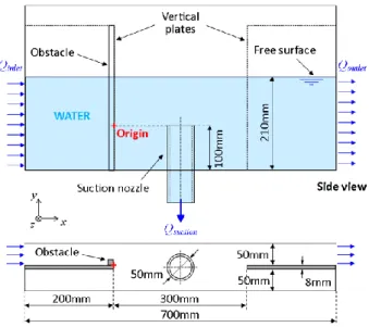
The length and width of the test section are respectively 700mm and 108mm. The height of the free surface is 210mm. Figure 1 gives a sketch of the test section of the rig which is named BANGA.
To separate the main free surface flow from a stagnant water area, two vertical plates (300mm apart) are placed in
the middle of the channel so that inlet and outlet flows are limited to the half of the channel cross-section. To induce a secondary down-flow, some water is pumped through a suction nozzle. The diameter of the nozzle, noted 𝐷, is of 50mm and it is set at 100mm height, i.e. 110mm below the free surface. The origin of the Cartesian frame is set on the border of the vertical plate at the height of the suction nozzle. The x axis coincides with the horizontal channel flow direction, y and z axis are the horizontal and vertical directions, respectively.
The present experimental set up is relatively close to that of Ezure et al., 2008 and Kimura et al., 2009. One of originality of this work is the possibility to introduce obstacles. These obstacles are mounted at the end of the first vertical plate as illustrated by the square in Figure 1. They produce different inlet flow conditions amenable to impact on the structure of the turbulent shear flow so as to provoke different conditions for gas entrainment.
Three geometries of obstacles are selected: square blocks (noted SB), half cylinders (noted HC) and ramps (noted RP). The square block and half cylinder are placed at the end of the vertical inlet Flat Plate (noted FP). The ramps are mounted along the flat platewith the highest part at its downstream end. Figure 2 illustrates these different Figure 1. Test section of the rig BANGA: The top picture is the side
view and the bottom one is the top view. The origin of the Cartesian frame is indicated with across. 𝑄𝑖𝑛 and 𝑄𝑜𝑢𝑡 denote the inlet and outlet
flow rates, respectively.
Page 3 sur 12 configurations with the obstacles. The height of the
obstacles, noted ℎ𝑜𝑏𝑠, are either 12.5mm or 25mm.
2.2.
Notations
The inlet and suction flow rates (in m3 h-1) are 𝑄𝑖𝑛 and 𝑄𝑠 respectively. The inlet and suction velocities are 𝑈𝑖𝑛 and 𝑉𝑠 respectively. 𝑈𝑜𝑏𝑠 is the velocity at the cross section perpendicular to the obstacles.
𝑈𝑖𝑛 = 𝑄𝑖𝑛 𝐿𝑖𝑛ℎ𝑤𝑎𝑡 , (1) 𝑉𝑠 = 𝑄𝑠 𝜋𝐷2/4 , (2) 𝑈𝑜𝑏𝑠= 𝑈𝑖𝑛 𝐿𝑖𝑛 𝐿𝑖𝑛− ℎ𝑜𝑏𝑠 , (3) where 𝐿𝑖𝑛 is the width of the inlet channel (50mm) and ℎ𝑤𝑎𝑡 is the water depth (210mm). For the flat plate configuration ℎ𝑜𝑏𝑠 = 0.
Similarly to Chang, 1979, the diameter 𝐷 of the suction nozzle is chosen as the reference length scale to build dimensionless numbers. In particular, the dimensionless coordinates are noted with a * so that: 𝑥∗= 𝑥 𝐷⁄ , 𝑦∗= 𝑦 𝐷⁄ and 𝑦∗= 𝑧 𝐷⁄ .
The inlet and suction Reynolds number, respectively noted 𝑅𝑒𝑖𝑛 and 𝑅𝑒𝑠, are defined as:
𝑅𝑒𝑖𝑛=𝑈𝑜𝑏𝑠𝐷
𝜈 , (4)
𝑅𝑒𝑠= 𝑉𝑠𝐷
𝜈 . (5)
where 𝜈 ≅ 10−6𝑚2𝑠−1 is the kinematic viscosity at 20°C. In order to underline the competition between the free surface flow and the downward flow in gas entrainment and surface swirl occurrence, two parameters, 𝜅 and 𝜉 are introduced: 𝜅 =𝑅𝑒𝑖𝑛 2 𝑅𝑒𝑠 . (6) 𝜉 = 𝑅𝑒𝑠 2 𝑅𝑒𝑖𝑛 . (7) Later on 𝜅 is used to study phenomena where 𝑅𝑒𝑖𝑛 has a stronger influence than 𝑅𝑒𝑠. In contrary, 𝜉 is used to describe phenomena where 𝑅𝑒𝑠 as a stronger influence than 𝑅𝑒𝑖𝑛.
2.3.
Measurements and processing
Flow measurements rely mainly on Particle Image Velocimetry (PIV) measurements to provide details about the inlet conditions, e.g. velocity profiles, and on flow visualization and processing to observe and quantify the gas entrainment phenomenon.
Particle Image Velocimetry (PIV) measurements (Raffel et al., 1998; Rossi et al., 2013) are performed using an Evergreen™ laser with double pulse laser sheets (thickness, wave length, duration and energy: 1mm, 532nm, 5ns, 120mJ). Double frames are recorded using a
PowerView™ Plus Charge Coupled Device (CCD) camera
of spatial resolution 4872 x 3248 pixels. The time lags of the double frames vary from 1ms to 2.5ms according to the flow rates. PIV computations are performed using Davis™ software from Lavision™. The final correlation windows are square windows of 48 pixels sides. An overlap of 50% is applied to build the velocity grid. Typical maximal displacements are about 10 pixels. The final instantaneous velocity fields are smoothed using a 3x3 mobile average.
The velocity fields are measured in the inlet area within horizontal and vertical planes. The vertical PIV planes are situated at y = 32mm and y = 37.5mm for 12.5mm size obstacles and the flat plate and for the 25mm side obstacles, respectively. These y values correspond to the middle position between the obstacles and the channel wall. The horizontal measurements are performed at z = 50mm (𝑧∗= 1) for all configurations. These latest measurements are performed from the side so as to avoid free surface deformations. To do so, the camera is set with an angle of 30° with the laser sheet. A calibration is applied to PIV frames to correct distortions using a reference grid and the ortho-rectification algorithm of DAVIS™ software.
Visualizations are performed in white backlighting with a Stemmer Imaging™ camera to observe surface swirl occurrence and gas entrainment phenomenon. Frames, with a spatial resolution of 2048 x 1088 pixels frames are acquired at 25Hz during 15min. The physical domain observed is 36cm long and 16 cm wide. It includes the free surface and the suction nozzle.
Image processing toolbox of Matlab™ is used to identify and quantify the occurrence of gas entrainment as follows:
1. The reference background, i.e. without gas entrainment, is subtracted to the original picture (Figure 3a) to improve the contrast. Such results are illustrated by Figure 3b.
2. The edges of the air areas are detected using the Canny method (Canny, 1986) evaluating the gray scale gradient. This step is illustrated in Figure 3c.
3. The edges are dilated to close opened contour. This step illustrated by Figure 3d.
4. The thick lines obtained are filled as illustrated in Figure 3e.
5. The filled shapes are eroded. This processing cleans the dilated border and removes the gray scale gradient of the free surface and the suction nozzle. This step is illustrated in Figure 3f.
6. Iso-countours are extracted (from the black and white image obtained) and are characterized as polygons so as to measure their geometrical characteristics. Resulting contours are illustrated in Figure 3g where they are superposed to the original picture.
Page 4 sur 12
2.4.
Flows explored
The Table 1 gives the flow rates, velocities and Reynolds numbers investigated.
Qin m3/h Uin m/s Qs m3/h Vs m/s Res Rein obstacles hobs FP 12.5mm 25mm 1.9 0.05 1.9 0.27 13 500 3 333 5 000 2 500 3.8 0.1 2.8 0.4 20 000 6 667 10 000 5 000 3.2 0.45 22 500 5.7 0.15 3.6 0.5 25 000 10 000 15 000 7 500 4.2 0.6 30 000 4.9 0.7 35 000 7.6 0.2 4.2 0.6 30 000 13 333 20 000 10 000 5.7 0.8 40 000 7.1 1 50 000 9.5 0.25 4.2 0.6 30 000 16 667 25 000 12 500 5.7 0.8 40 000 7.1 1 50 000
Table 1. Main flow parameters
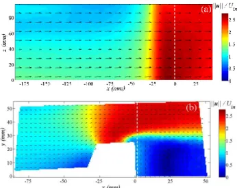
Figure 4 provides 2D dimensionless mean velocity field, averaged over 250 velocity fields, in the inlet area, ‖𝒖‖ 𝑈⁄ 𝑖𝑛, for the 25mm side square block; ‖𝒖‖ is the velocity amplitude. Figure 4a is measured at y = 37.5mm and Figure 4b2 is measured at z = 50mm. The two fields are in a good agreement. This highlights the reproducibility of the measurements since they are not made simultaneously. The black vectors indicate the direction of the flow. At the inlet, x < -50mm, the velocities are mainly parallel to the x-axis and their intensities are close to 𝑈𝑖𝑛 . For x > -25mm, the local speed increases due to the contraction of the test section. For x > 0, a strong transverse velocity gradient occurs between the inlet and the stagnant flows (Figure 4b). This generates a shear flow in the wake of the obstacle.
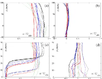
Figure 5 gives the dimensionless velocity profiles extracted along x = 0. The confidence interval at 95% of these mean velocity profiles is about 1%.
In the vertical plane, the vertical component (Figure 5b) is clearly negligible compared to the axial component (Figure 5a). In the horizontal plane, values of the transverse component (Figure 5d) above y = 25mm for 25mm side obstacles and y = 12.5mm for 12.5mm side obstacles are close to zero. Under these y values, the transverse component is more important due to the wake of obstacle and recirculation flow. Moreover, the axial velocity jumps in Figure 5c correspond to the position of the shear flows between the inlet and the “stagnant” flow. As for the velocity fields, a good agreement appears between the vertical and the horizontal velocity profiles of the axial component (Figure 5a and Figure 5c). The amplitudes of the velocity profiles are ordered similarly for the two sizes
2 Note that the boundaries of the velocity fields in Figure 4b are not straight because of the correction of the distortions.
Figure 3. Illustration of the different image processing steps: (a)
original image, (b) background subtraction, (c) edges detection, (d) edges dilatation, (e) filling closed contour, (f) erosion and (g) detected contours.
Figure 4. Dimensionless 2D temporal average, ‖𝒖‖ 𝑼⁄ 𝒊𝒏, in the
inlet area at y = 37.5mm (a) and z = 50mm (b). Experiments with the 25mm side SB, 𝑼𝒊𝒏= 𝟎. 𝟐𝟓𝒎 𝒔−𝟏 and 𝑽𝒔= 𝟏𝒎 𝒔−𝟏. Black
velocity vectors have a unit length to indicate the direction of the flow. White dashed lines represent the location of the profiles plotted in Figure 5.
Page 5 sur 12 of obstacles. The highest velocities are found for the inlet
configuration with the 25mm radius half cylinder.
The turbulence intensity levels range from 5% to 11% according to the inlet configurations. Table 2 gives more details so as to highlight the role of the obstacles in generating turbulence. 𝑈𝑖𝑛 m/s 𝑉𝑠 m/s SB HC RP FP 12.5mm size obstacles 0.1 0.45 9 8.6 7.7 9.5 𝑈𝑖𝑛 = 0.25𝑚/𝑠 𝑉𝑠 = 1 𝑚/𝑠 7.7 7.3 6.5 7.7 25mm size obstacles 𝑈𝑖𝑛 = 0.1𝑚/𝑠 𝑉𝑠= 0.45𝑚/𝑠 11.3 7.6 5.7 - 𝑈𝑖𝑛 = 0.25𝑚/𝑠 𝑉𝑠 = 1 𝑚/𝑠 8.1 6.5 4.8 -
Table 2. Turbulent intensities in percent within the inlet region. The velocities in the region of the suction nozzle are provided to complete the description of the experiments. Figure 6 gives the mean dimensionless velocity field, ‖𝒖‖ 𝑉⁄ , for the 12.5mm side square block in the vertical 𝑠 plane at y = 5mm. This plane is close to the centre-axis of the suction nozzle. The flow inside the suction nozzle is not symmetric. This indicates that it is sensible to the mean horizontal flow in the channel. In particular, a wake effect appears in left part, for −0.5 < 𝑥∗< 0, when the flow goes into the suction nozzle.
Velocity profiles are plotted in Figure 7a for the axial component and in Figure 7b for the vertical component
along the white dashed line represented in Figure 6. These profiles highlight the non-symmetrical distribution of the flow inside the suction nozzle. The suction velocity profiles are close to a plateau for −0.2 ≤ 𝑥∗≤ 0.4 with a ratio of the maximum of velocity to the mean velocity 𝑉𝑠 varying between 1.2 and 1.4.
3. Results and discussions
3.1.
Gas entrainmentmapping
Direct observations of the flow are performed to check if some gas is entrained or not. The onsets of gas entrainment are deduced from these observations.
The Figure 8 compares the present results with the ones obtained by Kimura et al., 2009 in the case of experiments with a flat plate. The results are close.
The Figure 9 provides gas entrainment mapping for the six obstacles according to the inlet velocity, 𝑈𝑖𝑛, and the suction velocity, 𝑉𝑠. When gas entrainment occurrences are observed the symbols are filled. The boundaries between the domains of gas entrainment and no gas entrainment are represented with red dashed lines. These thresholds change according to the shape and the size of obstacles. It is observed that the large obstacles trigger the occurrence of gas entrainment for lower suction velocities than for the small obstacles for a given 𝑈𝑖𝑛.
Figure 5. Dimensionless velocity profiles of (a) axial component
𝒖 𝑼⁄ 𝒐𝒃𝒔 and (b) vertical component 𝒘 𝑼⁄ 𝒐𝒃𝒔 are plotted at x = 0mm
in the vertical planes situated at y = 32mm for the 12.5mm side obstacles and the FP, and y = 37.5mm for the 25mm side obstacles (see Figure 4a). Dimensionless velocity profiles of (c) axial component 𝒖 𝑼⁄ 𝒐𝒃𝒔 and (d) transverse component 𝒗 𝑼⁄ 𝒐𝒃𝒔 are plotted
few mm after x = 0mm in the horizontal plane situated at z = 50mm (see Figure 4b). The SB, HC, RP and FP are plotted in black, blue, red and green color, respectively (see online version of this article for color coded version of this figure). Thin lines are used for 12.5mm size obstacles and heavy lines are used for 25mm size obstacles. Dashed lines correspond to 𝑼𝒊𝒏= 𝟎. 𝟏𝒎 𝒔−𝟏, 𝑽𝒔= 𝟎. 𝟒𝟓𝒎 𝒔−𝟏 and
solid lines correspond to 𝑼𝒊𝒏= 𝟎. 𝟐𝟓𝒎 𝒔−𝟏, 𝑽𝒔= 𝟏𝒎 𝒔−𝟏.
Figure 6. Dimensionless 2D temporal average, ‖𝒖‖ 𝑼⁄ 𝒊𝒏, in the vertical plane at y = 5mm, namely close to the center of the channel. Experiments with the 12.5mm side SB, 𝑼𝒊𝒏= 𝟎. 𝟐𝟓𝒎 𝒔−𝟏 and
𝑽𝒔= 𝟏𝒎 𝒔−𝟏. Black velocity vectors have a unit length to indicate
the direction of the flow. White dashed lines represent the location of the profiles plotted in Figure 7.
Figure 7. Dimensionless velocity profiles of (a) axial component
𝒖 𝑽⁄ and (b) vertical component 𝒘 𝑽𝒔 ⁄ are plotted at z = -15mm 𝒔
and y = 5mm. The 12.5mm size SB, HC, RP and FP are plotted in black, blue, red and green color, respectively (see online version of this article for color coded version of this figure). Dashed lines correspond to 𝑼𝒊𝒏= 𝟎. 𝟏𝒎 𝒔−𝟏, 𝑽𝒔= 𝟎. 𝟒𝟓𝒎 𝒔−𝟏 and solid lines
Page 6 sur 12 The thresholds of gas entrainment are summarized in Figure 10 for all experimental configurations including the flat platecase. The cases can be ranked according to the 𝑉𝑠 required to provoke gas entrainment for a given 𝑈𝑖𝑛. From the smallest to the highest 𝑉𝑠, this ranking is given in Table 3 along with the average ratio, noted ℜ𝑠, of the threshold suction velocities to the one of the flat plate configuration.
Position Obstacles ℜ𝑠 1 HC (ℎ𝑜𝑏𝑠 = 25𝑚𝑚) 0.7 2 SB (ℎ𝑜𝑏𝑠 = 25𝑚𝑚) 0.74 3 RP (ℎ𝑜𝑏𝑠 = 25𝑚𝑚) 0.84 4 RP (ℎ𝑜𝑏𝑠 = 12.5𝑚𝑚) 0.92 5 HC (ℎ𝑜𝑏𝑠= 12.5𝑚𝑚) 1 6 SB (ℎ𝑜𝑏𝑠 = 12.5𝑚𝑚) 1.1
Table 3. Threshold of obstacles ranked according to the mean ratio, 𝕽𝒔,
of the threshold suction velocity to the one of the flat plate case.
Increasing size of obstacles promotes gas entrainment and reverses the order of obstacles’ thresholds in term of suction velocity. In the case of the 12.5mm size obstacles, gas entrainment occurs with a smaller value of 𝑉𝑠 for the ramp than for the square block and the half cylinder. In the case of 25mm size obstacles, the ramp needs a higher value of 𝑉𝑠 to induce gas entrainment than for the half cylinder and the square block. Moreover, small obstacles trigger gas entrainment for suction velocity close to the flat plate since values of ℜ𝑠 are close to 1. However, increasing size of obstacles triggers gas entrainment for smaller 𝑉𝑠 than the flat plate configuration.
These results show that the occurrence of gas entrainment depends both, on the structure and on the intensity of the turbulent flow produced by the inlet conditions. The differences observed for different inlet Figure 8. Gas entrainment mapping for the flat plate configuration. The
present results are plotted with diamonds and the one from Kimura et al., 2009 are plotted with circles for water experiments and with triangles for sodium experiments. Symbols are filled when there is gas entrainment. The dashed line gives the threshold of gas entrainment occurrence for the present study and the solid line is 𝑸𝒊𝒏= 𝑸𝒔.
Figure 9. Gas entrainment mappings. SB of (a) 12.5mm and of (b)
25mm side; HC of (c) 12.5mm and (d) 25mm radius; RP of (e) 12.5mm and (f) 25mm height. Symbols are filled when gas entrainment occurs. The solid line indicates 𝑄𝑖𝑛= 𝑄𝑠.
Figure 10. The thresholds of gas entrainment are plotted with solid
lines and dashed lines for 𝒉𝒐𝒃𝒔 of 12.5mm and of 25mm respectively.
SB, HC and Ramps cases are highlighted using squares, circles and triangles, respectively. The dashed line without symbol is the FP case.
Page 7 sur 12 configurations may offer different test cases for MCFD
codes.
3.2.
Quantifications of gas entrainment and
surface swirls properties
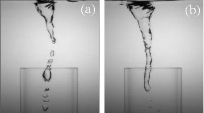
The two modes of gas entrainment observed are:
air bubbles are pumped through the suction nozzle3, a continuous surface swirl reaches the suction nozzle. Figure 11 illustrates these two observed modes for gas entrainment.
As the surface swirl is key to trigger gas entrainment, this subsection describes the geometrical properties of the surface swirl generated for the different flow configurations before discussing and quantifying the gas entrainment.
3.2.1. Geometrical characteristics of the surface swirls
The Figure 12 gives three snapshots which illustrate the positions of the surface swirls varying the inlet configurations. The surface swirls positions are upstream or downstream the centre of the suction nozzle according to the inlet configurations.
Using image processing, described in section 2.3. , the spatial positions of the surface swirls are measured at 𝑧∗= 2 (i.e. 10mm bellow the free surface level) and at
3
These bubbles are issued from the breaking of a surface swirls which results in a non-continuous surface swirl as illustrated in Figure 11a.
𝑧∗= 1 as highlighted by the dashed white lines in Figure 12.
The dimensionless position of the center of the surface swirls is introduced as:
𝑥𝑠𝑠∗ = (𝑥𝑠𝑠− 𝑥𝑛𝑜𝑧) 𝐷⁄ , (8) where 𝑥𝑠𝑠 and 𝑥𝑛𝑜𝑧 denotes the x-axis positions of the centres of the surface swirls and the suction nozzle, respectively.
The probability distributions of 𝑥𝑠𝑠∗ at 𝑧∗= 2are given in Figure 13 for different inlet configurations and flow intensities.
These distributions are not far from Gaussian distribution. The mean and the standard deviation of these positions’ distribution varies with the obstacles, 𝑅𝑒𝑖𝑛 and 𝑅𝑒𝑠. For the flat plate case (Figure 13a), the surface swirl tends to be downstream of the suction nozzle centre with 𝑥𝑠𝑠∗ ≥ 0. For the cases with obstacles the surface swirl tends to be upstream of the suction nozzle with 𝑥𝑠𝑠∗ ≤ 0. For the 12.5mm size obstacles, the highest probabilities are Figure 11. Illustration of gas entrainment through non-continuous (a)
and continuous (b) surface swirls. Associated videos can be found on the online version of the paper.
Figure 12. Illustration of continuous surface swirls for 25mm side SB
(a), 12.5mm side SB (b) and PP (c) with 𝑼𝒊𝒏 = 𝟎. 𝟐 𝒎 𝒔−𝟏 and
𝑽𝒔 = 𝟏𝒎 𝒔−𝟏. White dashed lines indicates planes 𝒛∗= 𝟐 and 𝒛∗= 𝟏.
Corresponding videos are available online.
(b)
(a)
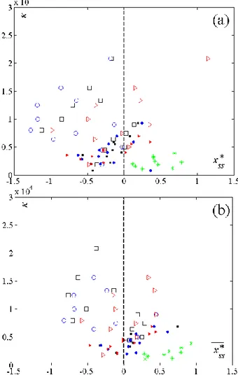
Figure 13. Probability distribution of the dimensionless positions of
centre of the surface swirls, 𝒙𝒔𝒔∗, at 𝒛∗= 𝟐. (a) FP; (b) and (c) SB of
sides 12.5mm and 25mm respectively; (d) and (e) HC of radius 12.5mm and 25mm respectively; (f) and (g) RP of height 12.5mm and 25mm respectively. Reynolds numbers, 𝑹𝒆𝒊𝒏, are indicated in the figures’
legend. Black solid lines and blue dashed lines correspond to 𝑹𝒆𝒔=
𝟐𝟐𝟓𝟎𝟎 and 𝟑𝟓𝟎𝟎𝟎, respectively. Red dotted lines and green dashed-dotted lines correspond to 𝑹𝒆𝒔= 𝟓𝟎𝟎𝟎𝟎.
(b)
(a)
Page 8 sur 12 observed around 𝑥𝑠𝑠∗ ≈ −0.5 for 𝑅𝑒𝑖𝑛 ≤ 13333. However,
for higher Reynolds numbers, they are around 𝑥𝑠𝑠∗ = 0. For the 25mm size obstacles, the highest probabilities locations are more sensitive to 𝑅𝑒𝑖𝑛 values than for 12.5mm size obstacles.
To complement the probability distributions of Figure 13, the temporal average of, 𝑥𝑠𝑠∗, noted 𝑥𝑠𝑠̅̅̅̅, and their ∗ standard deviations, /𝐷, are given for 𝑧∗= 2and𝑧∗= 1 in Figure 14.
The position 𝑥𝑠𝑠∗ is smaller for large obstacle than for small obstacle. For the inlet configurations with obstacles, 𝑥𝑠𝑠∗ tends to be negative for large obstacle at 𝑧∗= 2. The spreading of 𝑥𝑠𝑠∗ values is larger for 𝑧∗= 2 than for 𝑧∗= 1, in particular for the configuration with obstacles. This is due to the capture of the core of the surface swirls by the suction outlet as illustrated in Figure 12. It can be noted that for the configurations with small obstacles, 𝑥𝑠𝑠∗ tends to be negative for 𝑧∗= 2 and positive for 𝑧∗= 1. For the configuration without obstacles, 𝑥𝑠𝑠∗ > 0 for 𝑧∗= 1 and 𝑧∗= 2.
Figure 15 gives the dimensionless standard deviation of 𝑥𝑠𝑠∗, ∗=/𝐷, versus 𝜅 for 𝑧∗= 2 and 𝑧∗= 1. For the configurations with small obstacles and the flat plate, ∗ is found to increase with 𝜅. For the configurations with the large obstacles, ∗ seems to fluctuate around a mean value 〈𝜎∗〉. They are provided in Table 4 at two positions. Values increase from the flat plate (0.23) to the square blocks (0.4) at 𝑧∗= 2 and are ranked with the same order between the two obstacles’ size. Fluctuations are smaller for 𝑧∗= 1 than for 𝑧∗= 2.
These results highlight the fact the positions of the centres of the surface swirls strongly depend on the different flow configurations and their underlying turbulent structure. 12.5mm obstacles 25mm obstacles FP SB HC RP SB HC RP 𝑧∗= 2 0.4 0.35 0.34 0.4 0.36 0.3 0.23 𝑧∗= 1 0.2 0.25 0.21 0.25 0.27 0.23 0.17 Table 4. 〈𝝈∗〉 at 𝒛∗= 𝟐and 𝒛∗= 𝟏 for the configurations of Figure 15. Figure 14. The parameter 𝒙̅̅̅̅ is plotted in abscissa and 𝜿 in ordinate at 𝒔𝒔∗
(a) 𝒛∗= 𝟐 and (b) 𝒛∗= 𝟏. The 12.5mm and 25mm size obstacles are respectively plotted with filled and empty symbols. Squares, circles, triangles and stars are used for SB, HC, RP and FP inlet configurations respectively.
(a)
Figure 15. Plot of 𝜿 versus ∗ for 𝒛∗= 𝟐 (a) and 𝒛∗= 𝟏 (b). The configurations with 12.5mm and 25mm size obstacles are respectively plotted with filled and empty symbols. Squares, circles, triangles and stars are used for SB, HC, Ramps and FP cases respectively.
Page 9 sur 12 The thicknesses of the surface swirls are exported at
𝑧∗= 2 and 𝑧∗= 1 to build the Figure 16. It gives the average values of the dimensionless thicknesses, 𝐿𝑠𝑠∗ = 𝐿𝑠𝑠⁄ , versus 𝜅 𝜅𝐷 ⁄ . The parameter 𝜅𝑐 𝑐 is a critical value of 𝜅 identified as the transition between two regimes for the growth of 𝐿𝑠𝑠∗ . Its value is about 5500.
The configurations with the large obstacles generate the largest diameters and the one with the flat plate the smallest.
The thickness 𝐿∗𝑠𝑠 increases like power laws of 𝜅 𝜅⁄ , i.e. 𝑐 𝐿𝑠𝑠∗ ~(𝜅 𝜅𝑐⁄ )𝛽, when 𝜅 𝜅𝑐⁄ ≤ 1. The mean values of the exponents β are about 1 and 0.7 for 𝑧∗= 2 and 𝑧∗= 1 respectively. Fluctuation of the experimental points around these laws are typically about 8% at 𝑧∗= 2 and 16% at 𝑧∗= 1 which underline the good quality of this power law approximations. The exponents 𝛽 are estimated using least square approximations. They are given in Table 5 for the different flow configurations along with the normalized standard deviations of the experimental points around these laws. For 𝜅 𝜅𝑐⁄ ≥ 1, 𝐿𝑠𝑠∗ does not increase significantly with 𝜅 𝜅⁄ and it can be described as fluctuations around 𝑐 asymptotic values.
Here again, a notable difference appears between the flat plate and the obstacles at 𝑧∗= 2 since power 𝛽 of the flat plate configuration is twice lower than the other configurations. However, at 𝑧∗= 1, the values of 𝛽 are more homogenous between the different configurations.
12.5mm size obstacles 25mm size obstacles FP SB HC RP SB HC RP 𝑧∗= 2 0.98 0.76 1.4 0.93 0.88 1.1 0.5 disp % 11.3 6.4 12.1 17 3.2 2.8 5.7 𝑧∗= 𝟏 0.63 0.4 0.69 1.13 0.65 0.88 0.68 disp % 16.6 17.4 15.2 18.4 13.6 8 27 Table 5. Exponents of the power law approximation 𝑳𝒔𝒔∗~(𝜿 𝜿⁄ )𝒄𝜷 and
normalized standard deviations of the dispersion of the experimental points around these laws, noted disp, in percent.
3.2.2. Total area of the entrained gas
The total area, 𝐴𝑔𝑎𝑠, of the air entrained through the suction nozzle is measured for the different inlet configurations.
Given the depth of the suction nozzle (100mm) and the range of suction velocities (see Table 1), the 25Hz frequency of the camera is sufficient to capture all bubbles during their crossing of the suction nozzle. However, the air bubbles can collapse and change shape between to frames. This makes bubble tracking methods difficult to implement. Likewise, one difficulty to estimate 𝐴𝑔𝑎𝑠 is to count all the bubbles and to not count twice the same bubbles in two different frames. Taking into account the area of bubbles included in a subdomain of constant size introduce a bias in the measurement. In particular, considering the entire suction nozzle overestimates 𝐴𝑔𝑎𝑠 since bubbles are counting twice.
When the bubbles are crossing down the suction nozzle, two opposite forces/phenomena are applied to bubbles: the downward suction flow and the buoyancy force. Moreover, the flow is accelerated at the entrance of the suction nozzle before being quasi-established further downstream. This is particularly important for large bubbles that, for example, can sometimes enter the suction nozzle and leave it from the top without being entrained by the suction flow. Nevertheless, these events are never observed when the bubbles reach the bottom part of the suction nozzle. In consequence, the areas of the air bubbles are counted over a measurement domain starting from the bottom of the suction nozzle with a depth depending on the flow.
Between two frames the displacement of the bubbles is about 𝑉𝑏𝑢𝑏 ⁄ where 𝑉𝑓 𝑏𝑢𝑏 is the speed of the bubble and 𝑓 is the frequency of the camera. The domain of the suction nozzle where the area of bubbles is measured is adjusted to the flow conditions by roughly estimating 𝑉𝑏𝑢𝑏 ⁄ . To do 𝑓 so the suction velocity and the terminal velocity of a spherical bubble of equivalent diameter are used. Without the buoyancy effect, bubbles are considered to have a displacement about 𝛾 𝑉𝑠 ⁄ between to frames. The 𝑓 parameter 𝛾 is an empirical coefficient which relates the fact that the velocity is not uniform within the suction nozzle (see Figure 6 and Figure 7). For each suction velocity, 𝛾 is fixed according to the measured velocity profiles to 𝛾 = 1.25. The suction velocity is corrected by the terminal velocity, noted 𝑉𝑏𝑢𝑜𝑦. For each bubble, the value of 𝑉𝑏𝑢𝑜𝑦 is extracted from Haberman and Morton, 1953 as a function of the bubble radius 𝑟𝑏𝑢𝑏. The displacement considered for a bubble is then (𝛾𝑉𝑠 − 𝑉𝑏𝑢𝑜𝑦(𝑟𝑏𝑢𝑏)) 𝑓⁄ .
Hence, the area of a bubble, 𝒜𝑏𝑢𝑏, calculated in a frame is taken into account in 𝐴𝑔𝑎𝑠 calculation if the Figure 16. Dimensionless width of the surface swirls, 𝑳𝒔𝒔∗, versus 𝜿 𝜿⁄ 𝒄
with 𝜿𝒄≈ 𝟓𝟓𝟎𝟎. Measurements at 𝒛∗= 𝟐 and 𝒛∗= 𝟏 are separated
with a red dashed line. The inlet configurations with the 12.5mm and 25mm size obstacles are respectively plotted with filled and empty symbols. Squares, circles, triangles and stars are used for SB, HC, RP and FP cases respectively.
(b)
(a)
Page 10 sur 12 coordinates of its centre, 𝑧𝑏𝑢𝑏, is within the domain
𝑧𝑏𝑢𝑏≤ (𝛾𝑉𝑠 − 𝑉𝑏𝑢𝑜𝑦(𝑟𝑏𝑢𝑏)) 𝑓⁄ . The Figure 17 illustrates this measurement domain.
The total area of entrained air in a recorded frame is defined by:
𝐴𝑔𝑎𝑠= ∑ 𝒜𝑏𝑢𝑏 (9)
Figure 18 provides the dimensionless entrained gas area 𝐴𝑔𝑎𝑠⁄𝐷2 versus . The inlet configurations with obstacles entrain more air than the flat plate configuration. Among the cases with obstacles, the quantity of air pumped with large obstacles is greater than with small obstacles. In particular, for the two sizes, square blocks generate more entrained air than the half cylinder. The greater quantity of entrained air is induced by the large ramp whereas the smallest quantity of air is entrained by the small ramp, so that the ranking is inversed between the two sizes.
It can be observed that the large obstacles generate both larger surface swirls and higher quantity of entrained gas. Likewise, it is noticed that obstacles with a same size are ranked in the same way in term of threshold and entrained gas area.
Variation of dimensionless entrained gas area 𝐴𝑔𝑎𝑠⁄𝐷2 is approximated as power law 𝜉𝜃 fitted to the experimental measurements with the least square method. Adding obstacles change significantly gas entrainment behaviour since the slope of the flat plate is very larger than cases with obstacles (see Table 6).
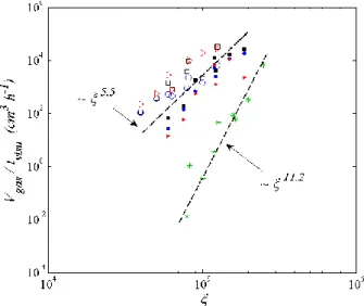
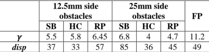
The total volume 𝑉𝑔𝑎𝑠 of entrained air is also estimated adding each measured bubble area to the power of 3/2: 𝑉𝑔𝑎𝑠 = ∑𝑁𝑖=1 𝒜𝑏𝑢𝑏3 2⁄ , with N the number of bubbles. The associated flow rate, 𝑉𝑔𝑎𝑠⁄𝑡𝑣𝑖𝑠𝑢, calculated on the visualisation time 𝑡𝑣𝑖𝑠𝑢 (15min), is plotted in Figure 19. As for the area 𝐴𝑔𝑎𝑠, experimental set of data are fitted with a power law 𝜉𝛾 which exponents are provided in Table 7.
As expected, values of 𝛾 in Table 7 differs from 𝜃3 2⁄ (Table 6) since the number of bubbles changes with 𝜉 and several size of bubbles are entrained.
12.5mm side obstacles 25mm side obstacles FP SB HC RP SB HC RP 𝜽 4.3 4.6 3.8 3.6 2.8 3.7 9.6 disp 32 34 56 63 33 48 47
Table 6. Exponents, 𝜽, of the approximated power laws giving the area of
entrained gas in function of 𝝃, i.e. 𝑨𝒈𝒂𝒔~𝝃𝜽 for the different inlet
configurations. disp is the dispersion (in %) of the experimental points around these power laws.
Figure 17. Illustration of the calculation of the entrained gas area
through the suction nozzle. Bubbles’ area is taking into account in 𝑨𝒈𝒂𝒔 when bubbles are placed under the white dashed line defined by 𝒛 = 𝒛𝒍𝒊𝒎 with 𝒛𝒍𝒊𝒎= (𝜸𝑽𝒔− 𝑽𝒃𝒖𝒐𝒚(𝒓𝒃𝒖𝒃)) 𝒇⁄ .
Figure 18. Dimensionless entrained gas area 𝑨𝒈𝒂𝒔⁄𝑫𝟐 versus . The inlet configurations with 12.5mm and 25mm size obstacles are respectively plotted with filled and empty symbols. Squares, circles, triangles and stars are used for SB, HC, RP and FP cases respectively.
(b)
(a)
Figure 19. Plot of entrained volume 𝑉𝑔𝑎𝑠 during visualization time
𝑡𝑣𝑖𝑠𝑢. The inlet configurations with 12.5mm and 25mm size obstacles
are respectively plotted with filled and empty symbols. Squares, circles, triangles and stars are used for SB, HC, RP and FP cases respectively.
Page 11 sur 12 12.5mm side obstacles 25mm side obstacles FP SB HC RP SB HC RP 𝜸 5.5 5.8 6.45 6.8 4 4.7 11.2 disp 37 33 57 85 36 45 49
Table 7. Exponents, 𝜸, of the approximated power laws giving the volume
𝑽𝒈𝒂𝒔 of entrained gas in function of 𝝃, i.e. 𝑽𝒈𝒂𝒔~𝝃𝜸 for the different inlet
configurations. disp is the dispersion (in %) of the experimental points around these power laws.
4. Conclusion
The objective of the present study is to investigate gas entrainment through an experimental set up in water. Since wakes of obstacles are expected to be present in Sodium cooled fast nuclear reactor, obstacles, with different shapes and sizes, are added at the channel inlet to produce various inlet conditions. These new results reveal the dependence of the gas entrainment to the triggers generating different structures of the turbulent flows for similar bulk properties,
i.e. flow rates. These results complement the existing
knowledge issued from the experiments using the flat plate configuration and open new perspectives.
The measurement of the suction velocity threshold required to provoke gas entrainment show that small obstacles behave similarly to the standard shear flow generated using the flat plate configuration. The configurations using the large obstacles tend to provoke gas entrainment for lower values of the suction velocity than the other configurations. Moreover, the ranked of the obstacles in terms of suction velocity required to entrain gas (at a given inlet velocity) is inversed between the two sizes of obstacles.
To study the details of the flow physical mechanisms, the occurrences and behaviour of the surface swirls are described. Moreover, in the context of nuclear safety for RNR-Na, it is important to quantify the volume of argon entrained in sodium through the heat exchanger. Then, an imaging processing tool is developed to detect the contour of surface swirl and entrained bubbles from shadowgraphy.
The different inlet configurations influence the width and the position of surface swirls. To our knowledge, the quantification of geometrical properties of the surface is a new result in the study of gas entrainment in open channel flow experiments. For the configuration with obstacles, they are larger and situated upstream from the suction nozzle. For the flat plate configuration the surface swirls are downstream the suction nozzle. It is found that for all cases, their widths vary with a power law of 𝜅. Surface swirl width increases with 𝜅 for small obstacles and the flat plate until a critical value of 𝜅 at 5500. From this value, it fluctuates around an asymptotic value for large obstacles.
The quantity of entrained gas is also estimated using a method taking into account suction velocity and buoyancy effect on bubbles. Here again, a power law of the entrained gas area was found. It implies the dimensionless parameter 𝜉 where the role of Reynolds numbers is inversed compared to the surface swirl width law. The flat plate
differs clearly from the cases with obstacles which are assembled around a same power. Number of bubbles change with values of 𝜉 and several sizes of bubbles are entrained through the suction nozzle.
To conclude, adding obstacles in the channel inlet area modifies significantly the gas entrainment and the surface swirl behaviour. In addition to provide new insights, it is expected that the detailed study of the configurations presented in this manuscript should offer interesting test cases for numerical codes validation.
5. Acknowledgements
This work is supported by the R4G program. The authors would like also to acknowledge Murielle Marchand, a CEA colleague, for her involvement in the development of BANGA experimental set up.
6. References
Baum, M.R., Cook, M.E., 1975. Gas entrainment at the free surface of a liquid: entrainment inception at a vortex with an unstable gas core. Nucl. Eng. Des. 32, 239–245. doi:10.1016/0029-5493(75)90133-8
Canny, J., 1986. A Computational Approach to Edge Detection. IEEE Trans. Pattern Anal. Mach. Intell.
PAMI-8, 679–698.
doi:10.1109/TPAMI.1986.4767851
Chang, E., 1979. Scaling law for air-entraining vortices. UB/TIB Hannover RR1519.
Cristofano, L., Nobili, M., Caruso, G., 2014. Experimental study on unstable free surface vortices and gas entrainment onset conditions. Exp. Therm. Fluid
Sci. 52, 221–229.
doi:10.1016/j.expthermflusci.2013.09.015
Eguchi, Y., Tanaka, N., 1994. Experimental study on scale effect on gas entrainment at free surface. Nucl. Eng. Des. 146, 363–371. doi:10.1016/0029-5493(94)90342-5
Eguchi, Y., Yamamoto, K., Funada, T., Tanaka, N., Moriya, S., Tanimoto, K., Ogura, K., Suzuki, T., Maekawa, I., 1994. Gas entrainment in the IHX vessel of top-entry loop-type LMFBR. Nucl. Eng. Des. 146, 373–381. doi:10.1016/0029-5493(94)90343-3
Ezure, T., Kimura, N., Hayashi, K., Kamide, H., 2008.
Transient Behavior of Gas Entrainment Caused by Surface Vortex. Heat Transf. Eng. 29, 659–666.
Ezure, T., Kimura, N., Miyakoshi, H., Kamide, H., 2011.
Experimental investigation on bubble characteristics entrained by surface vortex. Nucl. Eng. Des., 13th International Topical Meeting on Nuclear Reactor Thermal Hydraulics (NURETH-13) 241, 4575–4584. doi:10.1016/j.nucengdes.2010.09.021
Haberman, W.L., Morton, R.K., 1953. An experimental investigation of the drag and shape of air bubbles rising in various liquids (No. 802). David W. Taylor Model Basin.
Page 12 sur 12 Kimura, N., Ezure, T., Miyakoshi, H., Kamide, H., Fukuda,
T., 2009. Experimental Study on Gas Entrainment Due to Nonstationary Vortex in a Sodium Cooled Fast Reactor - Comparison of Onset Conditions Between Sodium and Water. Presented at the 17th International Conference on Nuclear Engineering, Brussels Belgium.
Kimura, N., Ezure, T., Tobita, A., Kamide, H., 2008.
Experimental Study on Gas Entrainment at Free Surface in Reactor Vessel of a Compact Sodium-Cooled Fast Reactor. J. Nucl. Sci. Technol. 45, 1053–1062. doi:10.1080/18811248.2008.9711892
Raffel, M., Willert, C., Kompenhans, J., 1998. Particle Image Velocimetry, Springer. ed.
Recoquillon, Y., 2013. Etude expérimentale et numérique des écoulements diphasiques dans la boîte à eau d’un véhicule automobile (PhD thesis). Orléans.
Recoquillon, Y., Andrès, E., Kourta, A., 2011a. Analyse et optimisation des écoulements diphasiques dans la boîte à eau d’un véhicule automobile. Presented at the 20ème Congrès Français de Mécanique, Besançon.
Recoquillon, Y., Kourta, A., Andrès, E., 2011b. Analyse des écoulements diphasiques dans la boîte à eau d’un véhicule automobile. Mécanique Ind. 12, 169–173. doi:10.1051/meca/2011110
Rossi, L., Doorly, D., Kustrin, D., 2013. Lamination, stretching, and mixing in cat’s eyes flip sequences with varying periods. Phys. Fluids 1994-Present 25, 073604. doi:10.1063/1.4812798
Takahashi, M., Inoue, A., Aritomi, M., Takenaka, Y., Suzuki, K., 1988. Gas Entrainment at Free Surface of Liquid, (I). J. Nucl. Sci. Technol. 25, 131–142. doi:10.1080/18811248.1988.9733568
Tenchine, D., 2010. Some thermal hydraulic challenges in sodium cooled fast reactors. Nucl. Eng. Des. 240, 1195–1217. doi:10.1016/j.nucengdes.2010.01.006
Tenchine, D., Fournier, C., Dolias, Y., 2014. Gas entrainment issues in sodium cooled fast reactors. Nucl. Eng. Des. 270, 302–311. doi:10.1016/j.nucengdes.2014.02.002
Vogt, T., Boden, S., Andruszkiewicz, A., Eckert, K., Eckert, S., Gerbeth, G., 2015. Detection of gas entrainment into liquid metals. Nucl. Eng. Des. 294, 16–23. doi:10.1016/j.nucengdes.2015.07.072