Extension of thermodynamic insights on batch extractive distillation to continuous operation

(1)

(2)

(3)

Abstract

We study the continuous extractive distillation of minimum and maximum boiling azeotropic mixtures A-B with a heavy or a light entrainer E, intending to assess its feasibility based on thermodynamic insights. The ternary mixtures belong to the 1.0-1a and 1.0-2 class ternary diagrams, each with two sub-cases depending on the univolatility line location. The column has three sections, rectifying, extractive and stripping. Differential equations are derived for each section composition, depending on operating parameters: distillate product purity and recovery, reflux ratio R and entrainer – feed flow rate ratio FE/F for the heavy case; bottom product purity and recovery, reboil ratio S and entrainer – feed flow rate ratio for the light entrainer case. For the case with a heavy entrainer fed as a boiling liquid above the main feed, the feasible product and operating parameters R and FE/F ranges are assessed under infinite reflux ratio conditions by using the general feasibility criterion enounced by Rodriguez-Donis et al. (Ind. Eng. Chem. Res, 2009, 48(7), 3544–3559). For the 1.0-1a class, there exists a minimum entrainer - feed flow rate ratio to recover the product, and also a minimum reflux ratio. The minimum entrainer - feed flow rate ratio is higher for the continuous process than for the batch because of the additional requirement in continuous mode that the stripping profile intersects with the extractive profile. For the 1.0-2 class both A and B can be distillated. For one of them there exists a maximum entrainer - feed flow rate ratio. The continuous process also has a minimum entrainer - feed flow rate ratio limit for a given feasible reflux ratio.

For the case with a light entrainer fed as saturated vapor below the main feed, the feasible product and operating parameters S and FE/F ranges are assessed under infinite reflux ratio conditions by using the general feasibility criterion enounced by Rodriguez-Donis et al. (Ind. Eng. Chem. Res, 2012, 51, 4643–4660), Compared to the heavy entrainer case, the main product is removed from the column bottom. Similar results are obtained for the 1.0-1a and 1.0-2 class mixtures whether the entrainer is light or heavy. With a light entrainer, the batch insight about the process feasibility holds for the stripping and extractive sections. Now, an additional constraint in continuous mode comes from the necessary intersection between the rectifying and the extractive sections.

This work validates the proposed methodology for assessing the feasibility of continuous extractive distillation processes and enables to compare entrainers in terms of minimum reflux ratio and minimum entrainer feed flow rate ratio.

Keywords

Extractive distillation – feasibility – thermodynamic insight – univolatility line - unidistribution line - reflux ratio – entrainer - feed flow rate ratio – reboil ratio – heavy entrainer – light entrainer

(4)

Résumé

Nous étudions la faisabilité du procédé de distillation extractive continue pour séparer des mélanges azéotropiques A-B à température de bulle minimale ou maximale, avec un tiers corps E lourd ou léger. Les mélanges ternaires A-B-E appartiennent aux classes 1.0-1-a et 1.0-2 qui se subdivisent chacune en deux sous-cas selon la position de la courbe d’univolatilité. La colonne de distillation a trois sections, rectification, extractive, épuisement. Nous établissons les équations décrivant les profiles de composition liquide dans chaque section en fonction des paramètres opératoires: pureté et taux de récupération du distillat, taux de reflux ratio R et rapport des débits d’alimentation FE/F dans le cas d’un tiers corps lourd; pureté et taux de récupération du produit de pied, taux de rebouillage S et rapport des débits d’alimentation FE/F dans le cas d’un tiers corps léger.

Avec un tiers corps lourd alimenté comme liquide bouillant au dessus de l’étage d’alimentation du mélange A-B, nous identifions le distillat atteignable et les plages de valeurs faisables des paramètres R et FE/F à partir du critère général de faisabilité énoncé par Rodriguez-Donis et al. (Ind. Eng. Chem. Res, 2009, 48(7), 3544–3559). Pour la classe 1.0-1a, il existe des rapports FE/F et reflux ratio minimum. Le rapport FE/F est plus important pour le procédé continu que pour le procédé discontinu parce que la faisabilité du procédé continu nécessite que les profils d’épuisement et extractifs s’intersectent. Pour la classe 1.0-2, les deux constituants A et B sont des distillats potentiels, l’un sous réserve que le rapport FE/F reste inférieur à une valeur limite maximale. Le procédé continu exhibe également une valeur minimale de FE/F à un taux de reflux ratio donné, contrairement au procédé discontinu.

Avec un tiers corps léger alimenté comme vapeur saturante sous l’étage d’alimentation du mélange A-B, nous identifions le produit de pied atteignable et les plages de valeurs faisables des paramètres S et FE/F à partir du critère général de faisabilité énoncé par Rodriguez-Donis et al. (Ind. Eng. Chem. Res, 2012, 51, 4643–4660). Comparé au cas des tiers corps lourds, le produit principal est obtenu en pied. Autrement, les comportements des classes 1.0-1a et 1.0-2 sont analogues entre les tiers corps léger et lourd. Avec un tiers corps léger, le procédé continu ajoute la contrainte que les profils de rectification et extractifs s’intersectent. La contrainte d’intersection des profils d’épuisement et extractif est partagée par les deux modes opératoires continu et discontinu.

Ce travail valide la méthodologie proposée pour évaluer la faisabilité du procédé de distillation extractive continue et permet de comparer les tiers entre eux en termes de taux de reflux ratio minimum et de rapport de débit d’alimentation minimal.

Mots-clés

Distillation extractive - courbes d’univolatilité - taux de reflux ratio - taux de solvent - entraîneur lourde - entraîneurlégerère

(5)

Acknowledgements

My deepest gratitude goes first and foremost to my supervisor Mr. Vincent GERBAUD, Chargé de recherche CNRS, for his constant encouragement and guidance. I really admire his wonderful and intriguing personality, his preciseness, patience, persistence, high requirements and great interest on research, his mind always abounded with new and effective idea, his courage to explore extensive different fields. He has walked me through all the stages of this thesis no matter weekends and evenings, without his consistent and illuminating instruction, this thesis would not have reached its present form.

I should like to acknowledge with deep gratitude the assistance and guidance given to me by Miss Hassiba BENYOUNES, lecturer of Université Des Sciences et Technologies. Oran, Algeria. I would also like to highlight the contribution of Ms. Ivonne Rodriguez-Donis, Prof. of Instituto Superior de Tecnologías y Ciencias Aplicadas, Cuba. It has been a pleasure collaborating with them and I sincerely appreciate their warm and cordial personalities. My heartfelt thanks are also due to their patience, encouragement, and professional instructions during my research activities.

I am also indebted to prof. Peter LANG of Budapest University of Technology and Economics, Faculty of Mechanical Engineering, Hungary, and prof. Jean Michel RENEAUME of Université de Pau et des Pays de l’Adour, France. Both of them are reviewers of this thesis. I thank them for spending time to give constructive suggestions, and kindly eliminate many of the errors in it, which are of help and importance in making the thesis a reality.

I am also honored by the presence of prof. Xavier JOULIA, co-founder and board member of Prosim Company who has so kindly accepted to be a part of the jury. Likewise, I would like to thank Mr. Michel MEYER, excellent professor of laboratoire de Génie Chimique, Dr. Olivier BAUDOUIN, head of process operation at Prosim. All of them have graciously accepted to be a member of the jury.

Last but not the least, my gratitude also extends to my dear colleagues and friends: Ali, Juliette, Sofia, Eduardo, Guillermo, László, Raul, Ferenc, ElAwady, Anthony，Moises, Meryem, Jean-Stephane, Fernando, René, Marco, Sayed, Nishant, Jesus, Marianne, Mary, Tibor, Adama, Marie, Mayra, Nguyen, Marie Roland and many others, without them I cannot have so happy, colorful, and wonderful life in France.

Weifeng SHEN Toulouse

(6)

i

Chapter Content

1. GENERAL INTRODUCTION ... 1

GENERAL INTRODUCTION ... 2

2. STATE OF THE ART, METHODOLOGY, OBJECTIVES ... 7

2.1 INTRODUCTION ... 8

2.2 PHASE EQUILIBRIUM ... 8

2.2.1 Phase equilibrium equations ... 8

2.2.2 Activity coefficient model ... 9

2.2.3 Non ideality of the mixture ... 11

2.2.4 Residue curve ... 13

2.2.5 Unidistribution and relative volatility ... 14

2.2.6 Ternary VLE diagrams classification ... 19

2.3 THE DISTILLATION PROCESS AND ITS IMPROVEMENT ...22

2.3.1 Highly integrated distillation columns ... 23

2.3.2 Vapor recompression distillation ... 24

2.3.3 Petlyuk arrangements ... 25

2.4 NONIDEAL MIXTURES SEPARATION ...26

2.4.1 Pressure-swing distillation ... 27

2.4.2 Azeotropic distillation ... 29

2.4.3 Reactive distillation ... 30

2.4.4 Salt-effect distillation... 31

2.4.5 Extractive distillation ... 31

2.5 LITERATURE STUDIES ON EXTRACTIVE DISTILLATION ...32

2.5.1 Extractive Batch Column configurations... 32

2.5.2 Continuous Column configurations ... 34

(7)

ii

2.5.4 Key operating parameters ... 36

2.6 METHODOLOGY FOR EXTRACTIVE DISTILLATION PROCESS FEASIBILITY IN RESEARCH ...36

2.6.1 Ternary systems studied in extractive distillation ... 37

2.6.2 Batch extractive process operation policies and strategy ... 41

2.6.3 Thermodynamic insight on extractive distillation feasibility ... 45

2.6.4 Topological features related to process operation ... 46

2.6.5 Extractive process feasibility assessed from intersection of composition profiles and differential equation ... 53

2.6.6 Extractive process feasibility from pinch points analysis ... 54

2.6.7 Feasibility validation by rigorous simulation assessment ... 56

2.7 RESEARCH OBJECTIVES ...57

3. EXTENSION OF THERMODYNAMIC INSIGHTS ON BATCH EXTRACTIVE DISTILLATION TO CONTINUOUS OPERATION. AZEOTROPIC MIXTURES WITH A HEAVY ENTRAINER ... 61

3.1 INTRODUCTION ...62

3.2 COLUMN CONFIGURATION AND OPERATION ...62

3.3 FEASIBILITY STUDY METHODOLOGY ...63

3.3.1 Thermodynamic feasibility criterion for 1.0-1a and 1.0-2 ternary diagram classes. ... 63

3.3.2 Computation of section composition profiles ... 66

3.3.3 Methodology for assessing the feasibility. ... 68

3.4 RESULTS AND DISCUSSION ...70

3.4.1 Separation of minimum boiling temperature azeotrope with heavy entrainers (Class 1.0-1a). ... 70

3.4.2 Separation of maximum boiling temperature azeotropes with heavy entrainers (class 1.0-2). ... 83

3.5 CONCLUSIONS ...96

4. EXTENSION OF THERMODYNAMIC INSIGHTS ON BATCH EXTRACTIVE DISTILLATION TO CONTINUOUS OPERATION. AZEOTROPIC MIXTURES WITH A LIGHT ENTRAINER ... 95

4.1 INTRODUCTION ... 100

4.2 STATE OF THE ART WITH LIGHT ENTRAINER ... 101

4.3 COLUMN CONFIGURATION AND OPERATION ... 103

4.4 EXTRACTIVE DISTILLATION FEASIBILITY ASSESSMENT ... 104

4.5 FEASIBILITY STUDY METHODOLOGY ... 106

4.5.1 Thermodynamic feasibility criterion for 1.0-1a and 1.0-2 ternary diagram classes. ... 106

(8)

iii

4.6 RESULTS ... 116

4.6.1 Separation of Maximum Boiling Temperature Azeotropes with light Entrainers (Class 1.0-1a). ... 116

4.6.2 Separation of Minimum Boiling Temperature Azeotropes with Light Entrainers (class 1.0-2). ... 127

4.7 CONCLUSIONS ... 138

5. CONCLUSIONS, PERSPECTIVE ... 143

5.1 CONCLUSIONS ... 144

5.2 PERSPECTIVE ... 150

6. APPENDIX: NOMENCLATURE, REFERENCE ... 151

6.1 NOMENCLATURE... 152

(9)

iv

Figure content

Figure 2.1. Typical homogeneous mixtures without azeotrope ... 11 Figure 2.2. Typical homogeneous mixtures with maximum boiling azeotrope, a negativedeviation from Raoult’s

law ... 12 Figure 2.3. Typical homogeneous mixtureswith minimum boiling azeotrope, a positive deviation fromRaoult’s

law ... 12 Figure 2.4. Typical homogeneous minimum boiling heteroazeotrope ... 12 Figure 2.5Condition of tangency between a residue curve and its corresponding distillate curve. ... 14 Figure 2.6 Feasible patterns of the VLE functions for binary mixtures of components 1 and 2: (a) equilibrium line

y(x), (b) distribution coefﬁcients Ki(x) and Kj(x),(c) relative volatility αij(x) and (d) distribution coefﬁcient

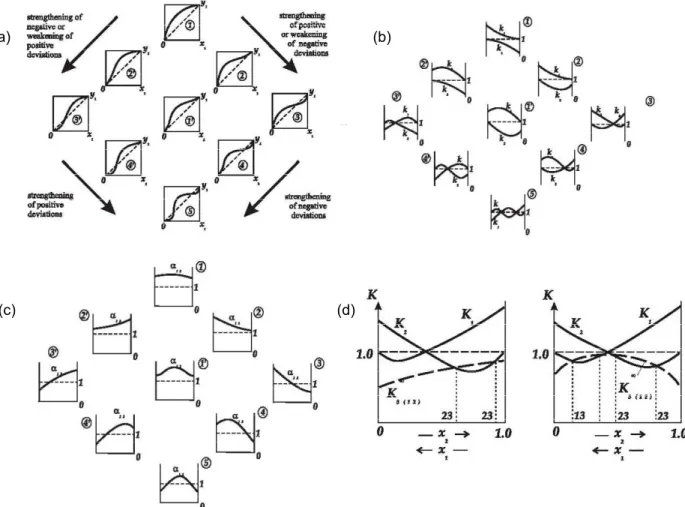
trajectories for a mixture 1-2-3 with minimum-boiling azeotrope 1-2 (Kiva et al., 2003). ... 17 Figure 2.7 Unidistribution and univolatility line diagrams for the most probable classes of ternary mixtures

according to Reshetov’s statistics (Kiva et al., 2003). ... 18 Figure 2.8 Azeotropic ternary mixture: Serafimov’s 26 topological classes and Reshetov’s statistics (Hilmen et al.,

2002). (o) unstable node, (∆) saddle, (●) stable... 20 Figure 2.9 Occurrence of classes from published data for ternary mixtures based on Reshetov’s statistics

1965-1988 (Kiva et al., 2003). ... 21 Figure 2.10 Ternary zeotropic mixtures Classes of diagrams of K-ordered regions for unilateral and bilateral

univolatility α-lines, respectively; 123, 132, 213, …, indices of K-ordered regions. ... 22 Figure 2.11. (a) Schematic diagram of HIDiC (Fukushima et al., 2006) and (b) HIDiC concentric tube column

(From PSE's Gproms manual, gP-B-611--051028 DR) ... 23 Figure 2.12 Schematic diagram of (1) direct vapor recompression distillation (1: distillation column, 2:

compressor, 3: reboiler–condenser and 4: expansion valve) and (2) external vapor recompression distillation (1: distillation column, 2,3: heat exchangers, 4: compressor and 5: expansion valve). (from

Jogwar and Daoutidis, 2009). ... 24 Figure 2.13 Schematic diagram of the fully thermally coupled (Petlyuk) arrangement (a)replaces the

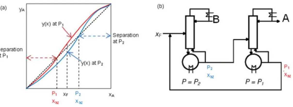
conventional arrangements with a prefractionator and a main column, and only a single reboiler and a single condenser is needed and (b) dividing wall configuration by moving the prefractionator into the same shell (from Halvorsen and Skogestad, 2011). ... 25 Figure 2.14 Effect of pressure on the azeotropic composition and corresponding continuous pressure-swing

distillation processes (from Gerbaud and Rodriguez-Donis, 2010). ... 28 Figure 2.15 Indirect separation (a) and direct (b) azeotropic continuous distillation under finite for a 1.0-2 class

(10)

v

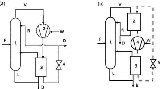
Figure 2.16 Configurations of extractive batch distillation column in rectifier and stripper ... 33 Figure 2.17. Flowsheet of typical extractive distillation with (a) heavy entrainer and (b) light entrainer ... 34 Figure 2.18 Configurations for the heterogeneous distillation column considering all possibilities for both the

entrainer recycle and the main azeotropic feed. (from Rodriguez-Donis et al. 2007) ... 35 Figure 2.19 Topological features related to extractive distillation process operation of class 1.0-1a when using a

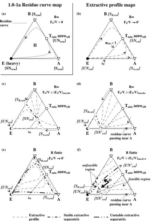
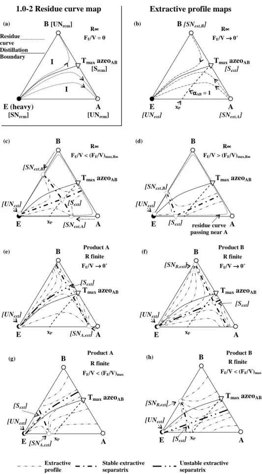
heavy entrainer (Rodriguez-Donis et al., 2009a). ... 47 Figure 2.20 Topological features related to the extractive distillation process operation of class 1.0-2 when using

a heavy entrainer. ... 52 Figure 2.21 The equilibrium stage: (a) component mass flows and (b) stream energy flows ... 56 Figure 3.1Configurations of extractive distillation column: (a) continuous (b) batch. ... 63 Figure 3.2Thermodynamic features of 1.0-1a mixtures with respect to batch extractive distillation. Separation of

a minimum boiling azeotrope with a heavy entrainer. ... 64 Figure 3.3Thermodynamic features of 1.0-2 mixtures with respect to batch extractive distillation. Separation of

a maximum boiling azeotrope with a heavy entrainer. ... 65 Figure 3.4Separation of acetone-heptane using toluene: (a) 1.0-1a class residue curve map (rcm) and batch

extractive profile map (b) (FE/V=0.01, R∞) (c) (FE/V=1,R∞) and (d) (FE/V=1,R=10). ... 71

Figure 3.5 Extractive distillation of acetone – heptane with toluene (1.0-1a class). Entrainer - feed flow rate ratio as a function of the reflux ratio. ... 72 Figure 3.6Extractive distillation of acetone – methanol with water (1.0-1a class). Entrainer - feed flow rate ratio

as a function of the reflux ratio to recover 98%mol acetone (A). ... 74 Figure 3.7Rectifying, extractive and stripping composition for four operating parameter points taken from

Figure 3.5 (b) point YU1, (b) point YF1, (c) point YU2 and (d) point YU3 ... 75

Figure 3.8Rigorous simulation result to recover acetone at FE/F=1, R=20 and FE/F=20, R=20, compared with

calculated profiles: (a-d) stripping section, (b-e) extractive section and (c-f) rectifying section. ... 77 Figure 3.9Separation of acetone-methanol using chlorobenzene: (a) 1.0-1a class residue curve map (rcm) and

batch extractive profile map (b) (FE/V=0.01, R∞) (c) (FE/V=2, R∞) and (d) (FE/V=2, R=5). ... 79

Figure 3.10Extractive distillation of acetone – methanol with chlorobenzene (1.0-1a class). Entrainer - feed flow rate ratio as a function of the reflux ratio to recover 98%mol methanol (B). ... 80 Figure 3.11 Rectifying, extractive and stripping composition for two operating parameter points taken from

Figure 3.10 (b) point YF1 and (b) point YU1 ... 81

Figure 3.12 Rigorous simulation result to recover methanol at: (a) R=1, FE/F=10; (b) R=1, FE/F=20; (c) R=20,

FE/F=10 and (c) R=20, FE/F=20. ... 83

Figure 3.13 chloroform-vinyl acetate using butyl acetate: (a) 1.0-2 class residue curve map (rcm) and batch

extractive profile map (b) (FE/V=0.1< (FE/V)max, R=15) ... 84

Figure 3.14Extractive distillation of chloroform – vinyl acetate with butyl acetate (1.0-2 class). Entrainer - feed

(11)

vi

Figure 3.15Comparison of three different entrainers to recover Chloroform (A) from the mixture chloroform – vinyl acetate. (a) Univolatility curve location. (b) Toluene, (c) Cyclohexane and (d) Butyl acetate feasible

regions. ... 87 Figure 3.16Extractive distillation of chloroform – vinyl acetate with butyl acetate (1.0-2 class). Entrainer - feed

flow rate ratio as a function of the reflux ratio to recover 98%mol vinyl acetate (B). ... 88 Figure 3.17Rigorous simulation result to recover vinyl acetate (B) at FE/F=5, R=5 and FE/F=0.1, R=5, compared

with calculating profiles: (a-d) stripping section, (b-e) extractive section and (c-f) rectifying section. ... 89 Figure 3.18acetone-chloroform using benzene: (a) 1.0-2 class residue curve map (rcm) and batch extractive

profile map (b) (FE/V=0.1 < (FE/V)max, R=60). ... 91

Figure 3.19 Extractive distillation of acetone – chloroform with benzene (1.0-2 class). Entrainer - feed flow rate

ratio as a function of the reflux ratio to recover 98%mol acetone (A)... 93 Figure 3.20 Extractive distillation of acetone – chloroform with benzene (1.0-2 class). Entrainer - feed flow rate

ratio as a function of the reflux ratio to recover 98%mol chloroform (B). ... 94 Figure 3.21Rectifying, extractive and stripping composition for four operating parameter points taken from

Figure 3.20 (a) point YU1, (b) point YF1, (c) point YU2 and (d) point YU3. ... 95

Figure 4.1 Configurations of extractive distillation column: (a) batch (b) continuous. ... 104 Figure 4.2.Thermodynamic features of 1.0-1a mixtures with respect to batch extractive distillation. Separationof

a maximum boiling azeotrope with a light entrainer. ... 106 Figure 4.3. Thermodynamic features of 1.0-2 mixtures with respect to batch extractive distillation. Separation of

a maximum boiling azeotrope with a light entrainer. ... 108 Figure 4.4. 1.0-1a class residue curve map of propanoic acid – DMF maximumn boiling azeotrope separation

using light entrainer MIBK. ... 117 Figure 4.5. Entrainer - entrainer - feed flow rate ratio FE/F as a function of the reboil ratio S. Propanoic acid –

MIBK – DMF Separation to recover A (propanoic acid). ... 118 Figure 4.6. The influence of the reboil ratio on stripping section composition profiles. ... 119 Figure 4.7.Operating parameter scene explanation.Points taken from Figure 4.5: (b) point YF1, (a) point YU1, (c)

point YF2 and (d) point YU2. ... 121

Figure 4.8. Rigorous simulation result to recover A (propanoic acid) at FE/F=1, S=15, compared with calculated

profiles: (a) rectifying section, (b)extractive section and (c) stripping section. ... 123 Figure 4.9. 1.0-1a class residue curve map of water – ethylene diamine maximum boiling azeotrope separation

using light entrainer acetone. ... 126 Figure 4.10. Entrainer - entrainer - feed flow rate ratio FE/F as a function of the reboil ratio S. Water – EDA –

acetone separation to recover B (EDA). ... 126 Figure 4.11. 1.0-2 class residue curve map of ethanol - water minimum boiling azeotrope separation using light

entrainer methanol ... 129 Figure 4.12. Entrainer - entrainer - feed flow rate ratio FE/F as a function of the reboil ratio S.

(12)

vii

Figure 4.13. 1.0-2 class residue curve map of MEK – benzene minimum boiling azeotrope separation using light

entrainer acetone. ... 131

Figure 4.14. Entrainer - entrainer - feed flow rate ratio F_E/F as a function of the reboil ratio S. MEK-benzene-acetone seperation: (a) to recover A (MEK) (b) to recover B (benzene). ... 132

Figure 4.15 Operating parameter scene explanation. Points taken from Figure 13b: (a) point YF1, (b) point YU1 ... 133

Figure 4.16. Influence of the reboil ratio on the extractive section composition profiles. ... 135

Figure 4.17. Rigorous simulation result to recover MEK (a-c) or Benzene (d-f) at S=15, FE/F=1 compared with simplified composition profiles: (a-d) stripping section, (b-e) extractive section and (c-f) rectifying section. ... 136

Table content

Table 2.1 The most important literature concerning extractive distillation separation of binary azeotropic and low relative volatility mixtures in a batch rectifier with light, intermediate or heavy entrainer. ... 39

Table 2.2 The study case related to extractive distillation separation of binary azeotropic and low relative volatility mixture in a batch rectifier with light, intermediate or heavy entrainer. ... 40

Table 2.3. The operating steps and limiting parameters of extractive distillation in configuration BED-I separating binary azeotropic and low relative volatility mixture in a batch rectifier with light, intermediate or heavy entrainer (Varga, 2006). ... 43

Table 2.4. The operating stages and limiting parameters of azeotropic extractive distillation in configuration BES-I separating binary azeotropic and low relative volatility mixture in a batch rectifier with light, intermediate or heavy entrainer (Varga, 2006). ... 44

Table 2.5 Summary of possible systems studied in the PhD thesis manuscript. ... 59

Table 3.1 Operating parameters for all study cases. ... 69

Table 3.2 Column operating specifications for rigorous simulation... 70

Table 3.3 Operating parameters corresponding to Figure 3.5. ... 73

Table 3.5. Operating parameters corresponding to Figure 3.7a,b,c,d ... 76

Table 3.6 Operating parameters corresponding to Figure 3.8a,b,c. ... 78

Table 3.7 Operating parameters corresponding to Figure 3.8 d,e,f. ... 78

(13)

viii

Table 3.14. Operating parameters corresponding to Figure 3.20. ... 94

Table 3.15. Operating parameters corresponding to Figure 3.21... 96

Table 4.1. operating parameters for all case study involving possible products. ... 115

Table 4.2. Column operating specifications for rigorous simulation ... 116

Table 4.6 Operating parameters corresponding toFigure 4.10. ... 127

Table 4.8 Operating parameters corresponding to Figure 4.14a... 133

Table 4.9 Operating parameters corresponding to Figure 4.15a,b. ... 134

(14)

1. General introduction

C

HA

P

TE

R

1

(15)

2

G

ENERAL INTRODUCTION

Distillation is the most widely used industrial method for separating liquid mixtures in many chemical and other industry fields like perfumery, medicinal and processing. The first clear evidence of distillation can be dated back to first century AD. Being the leading process for the purification of liquid mixtures, distillation columns consume about 40% of the energy used to operate plants in the refining and bulk chemical process industries according the U.S Dept of Energy. Azeotropic and low relative volatility mixtures often occur in separating industry and their separation cannot be realized by conventional distillation. Extractive distillation is then a suitable alternative process. Extractive distillation has been studied for many decades with a rich literature. Some main subjects studied include: column with all possible configurations; process operation polices and strategy; process design, synthesis, optimization; determining separation sequencing; entrainer design and selection, feasibility studies and so on. Among those topics, feasibility is always a critical issue as it is necessary to assess process feasibility before making the design specifications. Feasibility studies also contribute to a better understanding of complex unit operations such as the batch extractive distillation.

Upon the feasibility study, the design of conventional and azeotropic distillation is connected to thermodynamics, in particular the volatility of each compound and azeotrope. Furthermore, residue curve maps analysis allows assessing the feasibility under infinite reflux ratio conditions with the finding of the ultimate products under direct or indirect split conditions. However, distillation runs under finite reflux ratio conditions and finding which products are achievable and the location of the suitable feed composition region is more complicated because we must consider the dependency of composition profile on reflux ratio. This affects the range of composition available to each section profiles, due to the occurrence of pinch points, which differ from the singular points of the residue curve map. The identification of possible cut under key parameters reflux ratio, reboil ratio and entrainer - feed flow rate ratio has been the main challenge for an efficient separation of azeotropic mixtures.

Extractive distillation is a powerful and widely used technique for separating azeotropic and low relative volatility mixtures in pharmaceutical and chemical industries. Given an azeotropic mixture A-B (with A having a lower boiling temperature than B), an entrainer E is added to interact selectively with the original components and alter their relative volatility, thus enhancing the original separation. It differs from azeotropic distillation by the fact that the third-body solvent E is fed continuously in another column position than feed mixture. For decades a single feasibility rule holds in industry: extractive distillation should be operated by

(16)

3

choosing a miscible, azeotrope, relatively non-volatile component. The solvent forms no new azeotrope and the original component with the greatest volatility separates out as the top (bottom) product. The bottom (top) product consists of a mixture of the solvent and the other component.

Combining knowledge of residue curve maps and of the univolatility and unidistribution curves location Rodriguez-Donis et al (2009a, 2009b, 2010, 2012a, 2012b) published a general feasibility criterion for extractive distillation under infinite reflux ratio. The volatility order is set by the univolatility curves. Using illustrative examples covering all sub cases, but exclusively operated in batch extractive distillation, those authors found that Serafimov’s classes covering up to 53% of azeotropic mixtures were suited for extractive distillation: 0.0-1 (low relative volatility mixtures), 1.0-1a, 1.0-1b, 1.0-2 (azeotropic mixtures with light, intermediate or heavy entrainers forming no new azeotrope), 2.0-1, 2.0-2a, 2.0-2b and 2.0-2c (azeotropic mixtures with an entrainer forming one new azeotrope). For all suitable classes, the general criterion under infinite reflux ratio could explain the product to be recovered and the possible existence of limiting values for the entrainer - feed flow rate ratio for batch operation: a minimum value for the class 1.0-1a, a maximum value for the class 1.0-2, etc. The behavior at finite reflux ratio could be deduced from the infinite behavior and properties of the residue curve maps, and some limits on the reflux ratio were found. However precise finding of the limiting values of reflux ratio or of the entrainer - feed flow rate ratio required other techniques.

The feasibility always relies upon the intersection for the composition profiles in the various column sections (rectifying, extractive, stripping). Whatever the operation parameter values (reflux ratio, flow-rates...), the process is feasible if the specified product compositions at the top (xD) and at the bottom (xW) of the column can be connected by a single or by a composite composition profile. Here in this thesis we use geometrical analysis to evaluate profile intersection but mathematical ones could be used as well.

Several column configurations can be used for extractive distillation both in batch and continuous. In batch mode, both batch extractive distillation (BED) and simple batch distillation (SBD) processes can be performed either in rectifier, or in middle-vessel column, or in stripping column. With a heavy entrainer fed above the main feed, the batch column is a rectifier, with an extractive and a rectifying section and the product is removed as distillate from the top. With a light entrainer here we quote and apply the batch stripper column from Rodriguez-Donis et al., (2011), the original binary mixture (A+B) is initially charged into the column top vessel and it is fed to the first top tray as a boiling liquid. Light entrainer is introduced continuously at an intermediate tray leading to two column sections: extractive and stripping section. In the

(17)

4

continuous process, we consider the classical configuration, with the entrainer fed above the main feed, giving rise to three sections, rectifying, extractive and stripping ones.

In extractive distillation, the entrainer is conventionally chosen as a heavy (high boiling) component, however, there are some cases when its use is not recommended such as if a heat sensitive or a high boiling component mixture has to be separated. Besides, different entrainers can cause different components to be recovered or recovered overhead in extractive distillation. Therefore finding potential entrainers is critical since an economically optimal design made with an average design using best entrainer can be much less costly, Theoretically, any candidate entrainer satisfying the feasibility and optimal criteria can be used no matter it is heavy, light, or intermediate entrainer. Literature studies on intermediate entrainer or light entrainer, even though not too much, validate this assumption.

The presentation of this work focuses on four chapters:

Chapter 2 is a literature review to present the state of the art on the extractive distillation. This chapter introduces several issues related to our thesis: phase equilibrium, ternary diagram classifications, the principles of distillation and its improvement studies, possible method to separate non ideal mixtures, the state of art on extractive distillation, the general methodology used in this thesis, the objective, and organization of the thesis are shown at the end of this chapter. As this thesis is mainly concerned with feasibility studies, the most important methods are discussed in this part.

In Chapter 3, a systematic study is performed for the extractive distillation separation of azeotropic mixtures with a heavy entrainer belonging to 1.0-1a and 1.0-2 classes. The occurrence of two types of A-B azeotropic mixtures (minimum or maximum boiling temperature) and of two possible intersection of the univolatility line αAB=1 with the binary sides gives rise to four sub cases. Firstly, the column configuration is discussed. Then, the section composition profiles equations are derived for a heavy entrainer. Then a methodology in three steps is presented. In step1, based on batch feasibility knowledge, the feasibility of batch and continuous separation is studied under finite reflux ratio and entrainer - feed flow-rate, Insights gained from the batch extractive distillation criterion are extended to the feasible operation of the continuous process, with focus on the product cut sequence and operating parameter limit values. In step 2, assuming a given product purity and recovery, the feasible ranges of values of the operating parameters, reflux ratio R and entrainer - feed flow rate ratio FE/F are determined for the batch and continuous processes, and compared with the help of diagrams FE/F vs. R in continuous mode and FE/V vs. R in batch mode.

(18)

5

Comparison of three entrainers leading to the same class of diagram and sub-case is performed to check that the feasible conditions ranges are entrainer dependent, in particular the minimum reflux ratio and the minimum entrainer entrainer - feed flow rate ratio. In step 3, rigorous simulations verify the results of step 2, by providing rigorous values of the product purity and recovery.

Chapter 4 focuses on the extractive distillation feasibility studies with a light entrainer to separate minimum or maximum boiling azeotropic mixtures. The corresponding ternary diagram belongs to the 1.0-1a and 1.0-2 Serafimov’s class. Knowledge of the residue curve map and of the location of the univolatility curve αAB=1 can help assess which product is removed in the distillate. Contrary to the heavy entrainer case (Chapter 3), the main product is removed from the column bottom. The batch extractive process is a stripping column and the continuous process considers that the entrainer is fed below the main feed. The heavy entrainer methodology is now adapted to the light entrainer case. The section composition profile equations are reformulated in terms of the reboil ratio S and entrainer - feed flow rate ratio FE/F, also considering the entrainer physical state (saturated vapor or boiling liquid). The analyses of each of the four sub cases follow the same three step methodology used in the previous chapter: section profiles and methodology used, thermodynamic feasibility criterion analysis, calculation of reboil ratio vs. entrainer feed flow rate ratio diagrams and rigorous simulation, discussion and conclusion.

The last chapter deals with conclusion and future studies that can be drawn. Appendix collected some definitions of common terms in extractive distillation, the table data used in result discussion.

(19)

(20)

2. State of the art, methodology, objectives

C

HA

P

TE

R

2

(21)

8

2.1 INTRODUCTION

We first recall phase equilibrium issues to introduce the concepts of residue curve map and their classifications along with the concepts of the volatility and distribution curves. Then we survey distillation processes and their use for the separation of non ideal mixtures. We insist on extractive distillation key literature and review methods used to assess the feasibility of this process.

2.2 P

HASE EQUILIBRIUM

2.2.1 Phase equilibrium equations

The phase equilibrium behavior is the foundation of chemical mixture components separation by distillation. The basic relationship for every component in the vapor and liquid phases of a system at equilibrium is the equality of fugacities in all phases. In an ideal liquid solution the liquid fugacity of each component in the mixture is directly proportional to the mole fraction of the component. However, because of the no ideality in the liquid solution of the systems studied in the following chapters, activity coefficient representing the deviation of the mixture from ideality methods are used to describe the liquid phase behavior. For the vapor phase, ideal gas behavior is assumed leading to the gas fugacity equal to the partial pressure. Thus the basic vapor-liquid equilibrium equation is modified as:

P y f f x f_il = _i

γ

_i _i0,l = _iv = _i (2.1)

With the liquid phase reference fugacity l i

f0, being calculated from:

0 0 0 , 0 , 0 ₍ _, ₎ i i i v i l i T P P f =

ϕ

θ

(2.2) Where v i0,

ϕ

is the fugacity coefficient of pure component i at the system temperature (T) and saturated

vapor pressure, as calculated from the vapor phase equation of state (for ideal vapor phase: v i0,

ϕ

=1 ).

0

i

P is the saturated vapor pressure of component i at the system temperature.

0

i

θ

is the Poynting correction for pressure exp( 1

∫

P_* 0, )

P l i i dP V RT .

(22)

9

At low pressures, the Poynting correction is near unity and can be ignored. Thus the overall vapor– liquid phase equilibrium (VLE) relationship for most of the mixture systems in the following chapters can be described as the following equation:

* i i i iP x P y =

γ

(2.3)

When setting the condition γi=1, equation (2.3) is the so-called Raoult's Law. The computation of the

liquid activity coefficient γi requires thermodynamic models given in the next section.

Calculation of the saturated vapor pressure for a pure component is needed in Equation (2.3) for the VLE relationship. The extended Antoine equation can be used to compute liquid vapor pressure as a function of the system temperature T:

i C i i i i j i i C T C T C T C T C C P 7 6 5 4 3 2 1 0 _ln ln + + + + + = (2.4)

Where C1i to C7i are the model parameters, model parameters for many components are available in the literature or from the pure component databank of the Aspen Physical Property System.

2.2.2 Activity coefficient model

The UNIFAC, UNIQUAC, Wilson, NRTL activity coefficient model are recommended methods for highly non ideal chemical systems, The UNIFAC, UNIQUAC, NRTL model can be used for VLE, LLE and LLVE applications while the Wilson model can only be used for VLE application. (Kontogeorgis and Folas, 2010, Vidal, 2003). We use the UNIFAC model in this study to predict the VLE of each of the mixtures studied. In each case it was verified that the UNIFAC predictions agreed with available experimental data (Gmehling et al., 2004). The UNIFAC model is a semi-empirical method for the prediction of non-electrolyte activity estimation in non ideal mixtures. It is constituted by two parts: a combinatorial C

i

γ and a residual

component R i

γ .For the molecule i, the equation for the UNIFAC model is:

R i C i i γ γ γ ln ln ln = + (2.5)

The combinatorial component of the activity C i

γ is contributed to by several terms in its equation, and is the same as for the UNIQUAC model

j j j i i i i j j j i i i i i i i i C i x l x q l t q t q q z x + − −

∑

+ + −

∑

=

θ

φ

θ

φ

γ

' ' ' ' ' '_ln ln 2 ln ln (2.6)

(23)

10 Where

∑

= k k k i i i x q x q θ _(2.7)

∑

= k k k i i i x q x q ' ' ' θ _(2.8)

∑

= k k k i i i x r x r φ _(2.9) i i i i r q r z l = ( − )+1− 2 (2.10) ) ln exp( ₂ ' ' T e T d T c a t _ij _ij _ij ij k k i =

∑

θ + + + (2.11) 10 = z (2.12)

The residual component of the activity R i

γ is due to interactions between groups present in the equation ( )

[

( )

]

∑

= Γ − Γ = m 1 k k ln ln v ln i k k i R i

γ

(2.13) Where ( )i k

Γ is the activity of an isolated group in a solution consisting only of molecules i,

                            −         − = Γ

∑

= = = m j m n nj n jk j m j jk j K Q 1 1 1 k 1 ln ln

ϕ

θ

ϕ

θ

ϕ

θ

(2.14) Where:

∑

= = _m n n n j j j Q X Q 1 x θ (2.15)

(24)

11

∑∑

∑

= = = = _c i m k i i k c i i i j j x v x v X 1 1 1 _(2.16)         − =         ₋ − = T a RT U Ujk kk jk jk exp exp

ϕ

(2.17)

2.2.3 Non ideality of the mixture

In most distillation systems, the predominant non ideality occurs in the liquid phase because of molecular interactions. Equation (2.3) contains the liquid phase activity coefficient of the component j. When chemically dissimilar components are mixed together (for example, oil molecules and water molecules), there exists repulsion or attraction between dissimilar molecules. If the molecules repel each other, they exert a higher partial pressure than if the mixture was ideal. In this case the activity coefficients are greater than unity (called a “positive deviation” from Raoult‘s law). If the molecules attract each other, they exert a lower partial pressure than in an ideal mixture. Activity coefficients are less than unity (negative deviations).Activity coefficients are usually calculated from experimental data or from the aforementioned models regressed on experimental data. Azeotropes occur in a number of non ideal systems. An azeotrope exists when the liquid and vapor compositions are the same (xi=yi) at a given azeotrope temperature. There are several types of azeotropes, Figure 2.1-Figure 2.4sketch typical phase graphical representations of the

VLE. xA and yA x Vapor Liquid y TB T TA z Tequilibrium xA and yA x Vapor Liquid y P0 B P P0 A Pequilibrium xA Pure A Pure B A rich in vapor phrase yA phase

(25)

12 xA and yA xazeo vapor liquid Tazeo T TB TA xA and yA xazeo vapor liquid Pazeo P0 B P0 A P xA Azeotrope Pure A Pure B A rich in vapor phrase B rich in vapor phrase yA KA>1 KA<1 KA=1 phase phase

Figure 2.2.Typical homogeneous mixtures with maximum boiling azeotrope, a negative deviation from Raoult’s law xA and yA Vapor Liquid T Tazeo xazeo TB TA xA and yA Vapor Liquid P Pazeo xazeo P0 B P0 A xA Azeotrope Pure A Pure B A rich in vapor phase B rich in vapor phase yA

Figure 2.3.Typical homogeneous mixtures with minimum boiling azeotrope, a positive deviation from Raoult’s law T x and y Azeotrope vapor Liquid-liquid xA Azeotrope Pure A Pure B A rich in vapor phase B rich in vapor phase yA

Figure 2.4.Typical heteroazeotrope mixtures with minimum boiling azeotrope

The left part of Figure 2.1-Figure 2.4shows a combined graph of the bubble and dew temperatures,

pressure and the vapor-liquid equilibrium phase mapping, which gives a complete representation of the VLE. In addition, the right part gives the equilibrium phase mapping y vs. x alone. Each of these diagrams uniquely characterizes the type of mixture. Negative deviations (attraction) can give a higher temperature boiling

(26)

13

mixture than the boiling point of the heavier component, called a maximum-boiling azeotrope (Figure 2.2).

Positive deviations (repulsion) can give a lower temperature boiling mixture than the boiling point of the light component, called a minimum boiling azeotrope (Figure 2.3).

2.2.4 Residue curve

A residue curve map (RCM) is a collection of the liquid residue curves in a simple one-stage batch distillation originating from different initial compositions. The RCM technique is considered as powerful tool for the flow-sheet development and preliminary design of conventional multi-component separation processes. It has been extensively studied since 1900.Using the theory of differential equations, Doherty and his colleagues (e.g. Doherty and Malone, 2001a) explored the topological properties of residue curve map (RCM) which are summarized in two recent articles (Kiva et al., 2003, Hilmen et al., 2002b). The simple RCM was modeled by the set of differential equations.

∗ − = i i i _x _y dh dx (2.18)

Where h is a dimensionless time describing the relative loss of the liquid in the still-pot and dh=dV/L.xi is the mole fraction of species i in the liquid phase, and yi is the mole fraction of species i in the vapor phase. The yi values are related with the xi values using equilibrium constants Ki.

The singular points of the differential equation are checked by computing the associated eigenvalues. Within anon-reactive residue curve map, a singular point can be a stable or an unstable node or a saddle, depending on the sign of the eigenvalues related to the residue curve equation.

For non-reactive mixtures, there are three stabilities:

• Unstable node (denoted [un] with a symbol of white circle): The singular point eigenvalues are all

positive. It has a boiling point that is the lowest of the region of distillation. The residue curves move away from the unstable node with increasing temperature.

• Stable node (denoted [sn] with a symbol of solid circle): Singular points whose own values are all

negative. It has a boiling point that is the highest of the region of distillation. The residue curves move towards the stable node. Moving away from stable node along a residue curve, the temperature is decreasing.

• Saddle point (denoted [s] with a symbol of triangle): Singular points are intermediate boiling temperature points, which have at least one eigenvalue positive and the other negative. Some

(27)

14

residue curves away from a saddle point decreasing temperature and others with increasing temperature.

Some significant properties of residue curves are the following:

1. The singular points of residue curves networks are either pure component or azeotropes.

2. The Stability of singular points is an unstable node, a saddle point or a node stable and it depends on their respective boiling temperature.

3. In a simple distillation (Rayleigh’s distillation), the product follows a sequence of decreasing temperature. Thus, the unstable node will be the first distillate, followed by the saddle point and finally the node stable.

4. The orientation of the residue curve, that is to say, the changing composition of the boiling liquid, is in line with increasing temperature from the unstable node to the stable node.

5. Under total reflux ratio, the composition profile in a packed distillation column exactly follows the residue curve. Thus, in a column of infinite length at total reflux ratio, the distillate is the unstable node (direct split) or the bottom product is the stable node (indirect split).

6. The residue curve equation indicates that the equilibrium vector (y - x) is tangent to the residue

curvet point x (Figure 2.5), hinting at the still path direction in simple distillation.

7. Each residue curve is related to a vapor in equilibrium, which is named the distillate curve. The vapor curve is always located on the convex side of the corresponding residue curve (Figure 2.5).

x

Distillate curve

y

Residue curve Tangent line

Figure 2.5Condition of tangency between a residue curve and its corresponding distillate curve.

8. Two residue curves do not intercept.

2.2.5 Unidistribution and relative volatility

The distribution coefficient and relative volatility are well-known characteristics of the vapor–liquid equilibrium. The distribution coefficient Ki is defined by

(28)

15 i j i x y K = (2.19)

Ki characterizes the distribution of component i between the vapor and liquid phases in equilibrium.

K_i=1 defines the unidistribution curve. The vapor is enriched with component i if K_i>1, and is impoverished

with component i if Ki<1 compared to the liquid. The higher Ki, the greater the driving force (yi-xi) and the easier the distillation. The ratio of the distribution coefficient of components i and j gives the relative volatility. The relative volatility is a very convenient measure of the ease or difficulty of separation in distillation. The volatility of component j relative to component is defined as:

i i j j ij x y x y / / = α (2.20)

The relative volatility characterizes the ability of component i to transfer (evaporate) into the vapor phase compared to the ability of component j. Component i is more volatile than component j if αij>1, and less volatile if αij<1. For ideal and nearly ideal mixtures, the relative volatilities for all pair of components are nearly constant in the whole composition space. The situation is different for non ideal and in particular azeotropic mixtures where the composition dependence can be complex.

A large value of relative volatility α implies that components i and j can be easily separated in a distillation column. Values of αij close to 1 imply that the separation will be very difficult, requiring a large number of trays and high reflux ratio (high energy consumption). For binary systems, the relative volatility of light to heavy component is simply calledα:

) 1 /( ) 1 ( y / x x y − − =

α

(2.21) x x y ) 1 ( 1+ − =

α

(2.22)

Where x and y are the mole fractions of the light component in the liquid and vapor phases

respectively. Rearrangement of equation (2.21) leads to the very useful y-x relationship equation (2.22) that

can be employed when αis constant in a binary system. If the temperature dependence of the vapor pressure of both components is the same, relative volatility αwill be independent of temperature. This is true for many components over a limited temperature range, particularly when the components are chemically similar. Distillation columns are frequently designed assuming constant relative volatility because it greatly

(29)

16

simplifies the vapor-liquid equilibrium calculations. Relative volatilities usually decrease somewhat with increasing temperature in most systems.

Unidistribution and univolatility line diagrams can be used to sketch the VLE diagrams and represent the geometry of the simple phase transformation trajectories. The qualitative characteristics of the distribution coefficient and relative volatility functions are typical approaches for the thermodynamic topological analysis. Kiva et al., (2003) considered the behavior of these functions for binary mixtures. The composition dependency of the distribution coefficients is qualitative and quantitative characteristics of the VLE for the given mixture. The patterns of these functions determines not only the class of binary mixture (zeotropic, minimum-or maximum-boiling azeotrope, or biazeotropic), but also the individual behavior of the given mixture, as it is shown in Figure 2.6.

(30)

17

(b) (a)

(c) (d)

Figure 2.6. Feasible patterns of the VLE functions for binary mixtures of components 1 and 2: (a) equilibrium line y(x), (b) distribution coefficients Ki(x) and Kj(x), (c) relative volatilityαij(x) and (d) distribution coefficient

trajectories for a mixture 1-2-3 with minimum-boiling azeotrope 1-2(Kiva et al., 2003).

The composition dependence of the distribution coefficients of a ternary mixture of components 1, 2 and 3 can be represented by three surfaces K1(x), K2(x) and K3(x). The system of unidistribution lines Ki(x)=1 was analyzed in the composition space:

• The existence of a binary azeotrope gives rise to two unidistribution lines, and the existence of a

ternary azeotrope gives rise to three unidistribution lines.

• The point of pure component i may (or may not) give rise to a unidistribution line of component i. • A given residue curve map corresponds to a given set of feasible diagrams of unidistribution lines.

In a similar way to the distribution coefficient, the relative volatility features can be represented by isovolatility lines. Then the system of univolatility lines where αij=1 was proposed. It is evident that the point of a binary azeotrope Azij gives rise to anαij univolatility line and that the point of a ternary azeotrope gives rise to the three univolatility lines(Kiva et al., 2003).

(31)

18

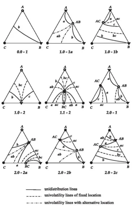
These features are represented in Figure 2.7 for the most probable classes (see the next section for the ternary diagram classification and probable occurrence).

Figure 2.7 Unidistribution and univolatility line diagrams for the most probable classes of ternary mixtures according to Reshetov’s statistics(Kiva et al., 2003).

Analysis of feasible diagrams of unidistribution and univolatility lines is given by Kiva et al., (2003). The main aim of their work was to consider feasible structures of the residue curve maps in more detail, and in fact this study helped to popularize more refined classification of the ternary diagrams. The diagrams of unidistribution lines were used as a main tool for analysis of tangential azeotrope and biazeotrope (Serafimov, 1996). Recently, Rodriguez-Donis et al (2009, 2010) studied how univolatility lines split the composition triangle into regions of certain order of volatility of components and defined a general feasibility

(32)

19

criterion for extractive distillation under infinite reflux ratio. In this work we consider unidistribution and univolatility line diagrams for the purpose of sketching the volatility order region and thus of assessing the feasible structures which will give possible products and offer information of possible limitation of entrainer feed.

2.2.6 Ternary VLE diagrams classification

The study of the thermodynamic classification of liquid-vapor phase equilibrium diagrams for ternary mixtures and its topological interpretation has a long history. Considering a ternary diagram A-B-E formed by a binary mixture A-B with the addition of an entrainer E, the classification of azeotropic mixtures in 113 classes was first proposed by Matsuyama (1978), then it was extended to 125 classes (Foucher et al., 1991a). After the work of Hilmen et al.(2002b), it became known that a more concise classification existed since the 70’s: Serafimov classification. As explained by Hilmen (2000), Serafimov extended the work of Gurikov and used the total number of binary azeotropes M and the number of ternary azeotropes T as classification parameters. Serafimov’s classification denotes a structure class by the symbol “M.T” where M can take the values 0, 1, 2 or 3 and T can take the values 0 or 1. These classes are further divided into types and subtypes denoted by a number and a letter. As a result of this detailed analysis, four more feasible topological structures, not found by Gurikov, were revealed. Thus Serafimov’s classification includes 26 classes of feasible topological structures of VLE diagrams for ternary mixtures. Both the classifications of Gurikov and Serafimov consider topological structures and thus do not distinguish between antipodal (exact opposite) structures since they have the same topology. Thus, the above classifications include ternary mixtures with opposite signs of the singular points and opposite direction of the residue curves (antipodal diagrams). Serafimov’s classification is presented graphically in Figure 2.8. The transition from one antipode to the other (e.g. changing from minimum-to maximum-boiling azeotropes) can be made by simply changing the signs of the nodes and inverting the direction of the arrows and the correspondence between Matsuyama and Serafimov’s classification is detailed in Kiva et al. (2003)and Hilmen (2000).

(33)

20

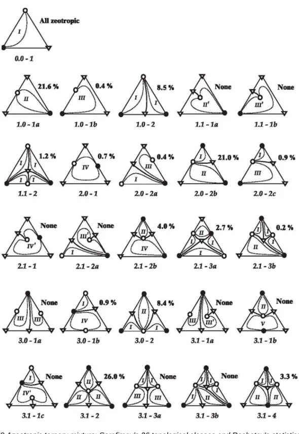
Figure 2.8 Azeotropic ternary mixture: Serafimov’s 26 topological classes and Reshetov’s statistics (Hilmen

et al., 2002). (o) unstable node, (∆_{) saddle, (}●_{) stable}

As illustrated in Figure2.7, the concentration simplex of these mixtures in the presence of an inf ection on conjugated tie and inverted tie lines consists of at least two regions characterized by different ranges for the phase equilibrium ratio Ki, where i is the component number. The region of the concentration simplex in

(34)

21

which the decreasing order of Ki remains the same concerning azeotrope ternary mixture was called the K-ordered region. These regions were separated from each other by univolatility α-lines.

The studies on the frequency of occurrences of different types of phase diagrams for ternary azeotropic mixtures were presented by Reshetov and Kravchenko (2007). All 26 Serafimov’s classes are topologically and thermodynamically feasible but their occurrence is determined by the probability of certain combinations of molecular interactions. The statistics on the physical occurrence of these 26 classes were provided to Kiva et al. (2003) by Reshetov (1998) but the original source is not available. The hereafter called “Reshetov’s statistics” are based on thermodynamic data for 1609 ternary systems from which 1365 are azeotropic. The database covers data published from 1965 to 1998. The results in Figure 2.8show that 16 out of the 26 Serafimov’s classes were reported in the literature. Although Reshetov’s statistics do not necessarily reflect the real occurrence in nature they can be used as an indicator of common azeotropic classes that are worthy of further investigation. A graphical representation of the occurrence of the various classes and types of ternary mixtures is given in Figure 2.9.

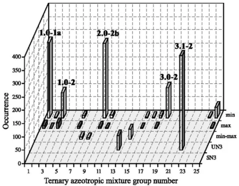
Figure 2.9 Occurrence of classes from published data for ternary mixtures based on Reshetov’s statistics 1965-1988 (Kiva et al., 2003).

The Figure 2.10 illustrates diagrams of K-ordered regions and their corresponding occurrence over the studied azeotrope mixtures classes found by the Reshetov and Kravchenko (2007).

(35)

22

1

3

2

3

1

2

3

1

2

3

1

2

3

1

2

3

1

2

3

1

2

3

1

2

3

1

2

3

1

2

3

1

2

3

1

2

3

1

2

3

1

2

3

1

2

3

1

2 Class 1

71.576%

Class 2

Class 3

Class 4

Class 5

Class 6

Class 7

Class 8

Class 11

Class 12

Class 16

Class 17

Class 18

Class 19

Class 27

Class 4a

0.127% 2.919% 11.294% 0.254% 1.269% 11.041% 0.254% 0.127% 0.254% 0.254% 0.127% 0.127% 0.127% 0.127% 0.127%

1

Figure 2.10 Ternary zeotropic mixtures Classes of diagrams of K-ordered regions for unilateral and bilateral

univolatility α_{-lines, respectively; 123, 132, 213, …, indices of K-ordered regions.}

2.3 T

HE DISTILLATION PROCESS AND ITS IMPROVEMENT

Distillation is the most widely used industrial method for separating liquid mixtures in many chemical and other industry fields like perfumery, medicinal and food processing, the first clear evidence of distillation can be dated back to first century AD (Forbes, 1970). Being the leading process for the purification of liquid mixtures, the distillation process is driven by the differences between the vapor and liquid phase

(36)

23

compositions of the mixture arising from successive partial vaporization and condensation steps (Geankoplis, 2003). Distillation operations are responsible for 40% of the energy used in the chemical process industries.

The technology that can significantly reduce the energy requirement will represent a major breakthrough, and give significant competitive edge to the companies that adopt it. Regarding its high energy consumption, which comes from the vaporization of the liquid and is related both to the mixture charge and to the reflux ratio inside the column, progress has been made by the use of HIDiC (highly integrated distillation columns) (Skogestad et al., 1992, 1997;Nakaiwa et al., 2001, 2003), vapor recompression column (Jogwar et al., 2009) and other Petlyuk-like columns (Wolff and Skogestad, 1995; Halvorsen and Skogestad, 1999; Vitoria et al.2008;Halvorsen and Skogestad, 2011).

2.3.1 Highly integrated distillation columns

Bottom product

(b)

(a)

2.3.2 Vapor recompression distillation

(b) (a)

Figure 2.12 Schematic diagram of (1) direct vapor recompression distillation (1: distillation column, 2: compressor, 3:reboiler–condenser and 4: expansion valve)and (2)external vapor recompression distillation (1:

distillation column, 2,3: heat exchangers, 4: compressor and 5: expansion valve).(From Jogwar and Daoutidis, 2009).

Vapor recompression distillation is an energy integrated distillation configuration which works on the principle of a heat pump. The vapor coming from the top of the distillation column is compressed in a compressor and is then used to transfer energy in a combined reboiler–condenser leading to the so-called direct vapor recompression distillation (Figure 2.12a). On the other hand, an external refrigerant can also be used to facilitate the energy transfer between the top vapor stream and the bottom liquid stream, leading to the so-called external vapor recompression distillation (Figure 2.12b).Direct vapor recompression is commonly used, whereas external vapor recompression is generally preferred when the column f uid is corrosive or is not a good refrigerant (Jogwar & Daoutidis 2009).

(38)

25

Muhrer et al. (1990) proposed a specific vapor recompression columns control scheme. Compared to conventional columns, heat input control was replaced by compressor control. The pressure loops were found to be faster than the composition loops. Hence, the pressure loop can be adjusted for relatively tight control independently from the composition loops. This simple conclusion can be universally used for most vapor recompression columns if they are satisfying their two requirements: the composition time constants of column must be 5 times larger than the pressure time constant, and the time constants of reboiler of conventional and vapor recompression columns should be nearly the same. For most columns vapor recompression distillation systems the two requirements can be satisfied. Jogwar & Daoutidis (2009) developed a systematic modeling framework which explicitly captures the difference between the different material and energy flows. A case of propane–propylene separation was considered to demonstrate the effectiveness of the proposed control strategy.

2.3.3 Petlyuk arrangements

Figure 2.13 Schematic diagram of the fully thermally coupled (Petlyuk) arrangement (a) replaces the conventional arrangements with a prefractionator and a main column, and only a single reboiler and a single

condenser is needed and (b) dividing wall configuration by moving the prefractionator into the same shell (from Halvorsen and Skogestad, 2011).

Petlyuk arrangements may reduce internal vapour flow rate ratio, and thereby the need for external heating and cooling. The basis for the configuration is the prefractionator arrangement in Figure 2.13, where the reboiler and condenser of the prefractionator column are removed and replaced with directly connected vapour and liquid streams. This is called a full thermallycoupled arrangement. The dividing wall column (DWC) is an implementation of the fully thermally coupled Petlyuk column arrangement (Petlyuk et al., 1965) in a single shell. Kaibel (1987) firstly introduced a distillation column with vertical partitions to separate a feed