Simple Median-Based Method for Stationary
Background Generation Using Background
Subtraction Algorithms
B. Laugraud, S. Piérard, M. Braham, and M. Van Droogenbroeck
INTELSIG Laboratory, University of Liège, Belgium
Abstract. The estimation of the background image from a video se-quence is necessary in some applications. Computing the median for each pixel over time is effective, but it fails when the background is visible for less than half of the time. In this paper, we propose a new method leveraging the segmentation performed by a background subtraction al-gorithm, which reduces the set of color candidates, for each pixel, be-fore the median is applied. Our method is simple and fully generic as any background subtraction algorithm can be used. While recent back-ground subtraction algorithms are excellent in detecting moving objects, our experiments show that the frame difference algorithm is a technique that compare advantageously to more advanced ones. Finally, we present the background images obtained on the SBI dataset, which appear to be almost perfect. The source code of our method can be downloaded at http://www.ulg.ac.be/telecom/research/sbg.
1
Introduction
Estimating the static background image from a video sequence has many inter-esting applications. Traditionally, the foreground (FG) is defined as objects or people moving in the front of the scene that form the background (BG). Note that a temporarily stopped FG object must be dissociated from the BG (e.g. a pedestrian waiting for a green light). An example of application is the rendering of non-occluded pictures of monuments, or landscapes, which are difficult to ob-serve in crowded places. Another example is the initialization of the background subtraction (BGS) algorithms [3] that aim at classifying, into a segmentation map, for each frame of a video sequence, pixels as belonging to the FG or the BG. BGS algorithms often assume that the few first frames are motionless, which leads to inappropriate segmentation maps for the beginning of the sequences if the assumption does not hold. In order to accelerate the initialization process, they could benefit from a better estimation of the initial BG image.
The SBMI challenge [8] aims at developing methods to estimate the BG image of a scene given a video sequence taken from a static viewpoint, but with potential jitter. To evaluate such methods, the SBI dataset [8], composed of 7 sequences, is provided. Their characteristics prevent the use of simple approaches such as taking the median color per pixel using all the frames (we refer to this
method as the MED method hereafter), as the BG may be visible in less than 50% of the frames for some pixels [7]. Also, for some sequences, there is no image void of occluding objects, although the BG color is visible for each pixel for at least a few frames. Heuristics used in inpainting techniques [10] might be useless in this context. The BG is assumed to be unimodal, this means that we do not have to consider effects due to dynamic textures or illumination changes in the BG, and that there is only one possible BG at each instant. Moreover, as all the sequences are quite short (they are between 257 and 499 frames long), one background image should suffice to represent the static background.
In this paper, we present a simple method to estimate the BG image. Instead of estimating the BG image to initialize BGS algorithms as discussed above, we rely on BGS algorithms to generate a reference image for the BG. One could think that it is sufficient to simply extract this image from the BG modeled by such an algorithm. However, this approach has major drawbacks. Among others, despite that some BGS algorithms build an internal BG image reference, they often have a more complex model (e.g. for the Mixture of Gaussians [13]) or even store samples (e.g. ViBe [2]). Thus, extracting a BG image from the model of a given BGS algorithm might be complicated due to the internal mechanisms involved in the model maintenance. Rather than trying to extract a reference im-age directly, our idea consists in detecting motion according to the segmentation maps produced by any BGS algorithm, and integrate this process into a generic framework. Note that the optimal BGS algorithm for video-surveillance might not be best for our purpose. For example, classifying shadowed areas in the FG would help us, but this is rarely the targeted behavior of BGS algorithms.
The paper is organized as follows. Section 2 describes the method proposed in this paper, and presents the related work. Our experiments and results are provided and discussed in Section 3. Section 4 concludes this paper.
2
Proposed method
According to Maddalena et al. [7], the stationary BG generation problem can be solved with the MED method when the BG is visible for half of the time. Unfortunately, for most sequences of the SBI dataset or also often in practice, this is not the case. Nevertheless, this simple idea combined to a BGS algorithm to select relevant frames, for each pixel, proves effective and produces excellent results. In our method, the median is computed on a per-pixel subset of frames
(of fixed size S), selected by considering the probability p∗+ of FG elements in
the neighborhood of the considered pixel, instead of the pixel only. For example, colors might be darkened in shadowed areas but still be undetected by some BGS algorithms. As casted shadows are spatially close to the associated objects,
the spatial estimation of p∗+helps discarding them. More specifically, to estimate
this probability, we divide the image plane in N × N non-overlapping patches, and compute the proportion of pixels classified in the FG class, by the BGS algorithm, for the patch containing the considered pixel. Note that we discard
the first frame processed by the BGS algorithm as the BGS model is undefined and this frame cannot be segmented.
In practice, all BGS algorithms require an initialization period during which their outputs are unreliable. The number of frames needed for the initialization is algorithm dependent, and can be larger than the number of available frames in the sequences of the SBI dataset. Therefore, we suggest to process the sequences several times. Let γ denote the total number of passes, which is chosen to be odd. The odd passes process the frames forwards, while the even ones process them backwards. Note that the idea of processing frames in a non chronological order to detect motion was first introduced in [14]. The internal model of the BGS algorithm is always updated, even during the last pass.
For each pixel, our method selects the S frames with the lowest probability
p∗+ of FG computed for the corresponding patch. The S frames are issued from
the ones processed during the γ passes, as we observed the trend that discarding the γ − 1 first passes deteriorates our results. In the case where S is too small to select all the frames with equal probabilities, we arbitrarily select the last ones encountered during the processing. Then, the BG color is estimated by taking the median of the colors in the S selected frames, the median being computed for the red, green, and blue components independently.
2.1 Related work
Following the terminology of Maddalena et al. in [7], our method is:
– Hybrid. We combine the pixel-level analysis of a background subtraction algorithm with a region-level selection process to extract patches with the highest background probabilities.
– Non-recursive. Our method stores colors observed in the previous frames in a buffer, and directly derives the estimated background image by means of a temporal median filter.
– Selective. The median is computed in each pixel on a selection of samples with high background probability.
To the best of our knowledge, the closest method of the literature has been proposed by Amri et al. [1]. Its main idea lies in the application of a median filter on a set of frames, selected according to a criterion based on motion analysis. However, this method presents significant differences with our one.
Among others, due to the different targeted application (constructing a wide panoramic image from a video sequence taken with a moving camera), the work of Amri et al. is much more complicated. Moreover, the authors propose an iterative method processing frames until a stopping criterion is achieved. And last but not least, instead of being detected by temporal analysis, the motion is detected with a comparison between each processed frame and the last esti-mated BG image. Note that such a comparison is made by using a hysteresis thresholding technique while a raw BGS algorithm is used in our method.
3
Experiments and results
Our proposed method has 4 parameters: the used BGS algorithm, the buffer size S, the amount of patches N ×N , and the number of passes γ. In our experiments, we have tested all combinations of 10 BGS algorithms, S ∈ {5, 11, 21, 51, 101, 201}, N ∈ {1, 3, 5, 10, 25, 50}, and γ ∈ {1, 3, 5, . . . , 19}. The chosen BGS algorithms are listed in Section 3.1. The metrics used to assess the estimated BG images are detailed in Section 3.2, and results are presented and discussed in Section 3.3.
3.1 Background subtraction algorithms
All BGS algorithms proceed at the pixel level. The most intuitive one, the frame difference (F. Diff.), is based on a simple motion detection method which applies a threshold to the distance of colors between consecutive frames.
As noise is not spatially and temporally uniform, other algorithms have been proposed to estimate the statistical distribution of background colors over time. Wren et al. [15] supposed a Gaussian noise, and modeled the background with a Gaussian distribution whose mean and variance are adapted constantly (Pfinder). Stauffer et al. extended this idea to handle dynamic backgrounds us-ing a mixture of Gaussians [13] (MoG G.). Zivkovic improved this by adaptus-ing the number of needed Gaussians over time [16] (MoG Z.). The Sigma-Delta al-gorithm (S-D) is another variant of Pfinder, proposed by Manzanera et al. [9], estimating the median (instead of the mean) based on a Σ − ∆ estimator.
As an alternative, El Gammal et al. [4] proposed, in their KDE algorithm (KDE), to build the distribution by applying Parzen windows on a set of past samples. ViBe (ViBe), proposed by Barnich et al. [2], uses a pure sample-based approach and random policies to sample, in a conservative way, the observed background values. Some variants have been developed by, among others, Hof-mann et al. [5] with PBAS (PBAS) by adding adaptive decision thresholds and update rates, and by St-Charles et al. [12] with SuBSENSE (SuBS.) by associ-ating these adaptive parameters with the sampling of LBSP strings.
Finally, an approach based on self organization through artificial neural net-works has been proposed by Maddalena et al. with the SOBS algorithm, whose idea is inspired from biologically problem-solving methods [6]. It should be noted that the implementations of the 10 used BGS algorithms are provided by the BGSLibrary [11] or by the authors.
3.2 The metrics used to assess the estimated background images
For each set of parameters, we have computed the eight metrics suggested by Maddalena et al. [8]. As two metrics are normalized versions of two others, we decided to keep only six of them: the Average Gray-level Error (AGE), the Per-centage of Error Pixels (pEPs) (a difference of values larger than 20 is considered as an error), the Percentage of Clustered Error Pixels (pCEPs) (any error pixel
whose 4-connected neighbors are also error pixels), the Peak-Signal-to-Noise-Ratio (PSNR), the Multi-Scale Structural Similarity Index (MS-SSIM) that es-timates the perceived visual distortion, and the Color image Quality Measure (CQM). The AGE, pEPs, and pCEPs are to be minimized, while the PSNR, MS-SSIM, and CQM are to be maximized. For any set of parameters, metric values were averaged over the 7 video sequences of the SBI dataset.
3.3 Results
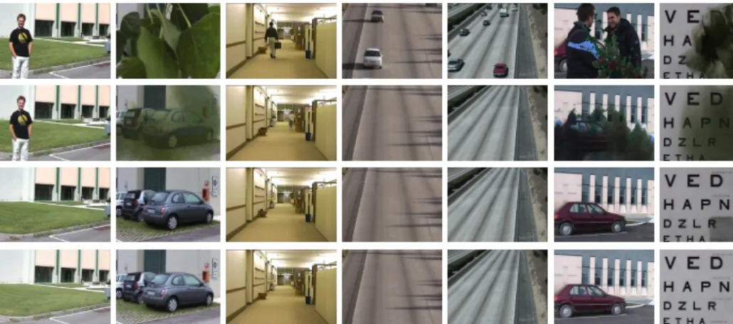
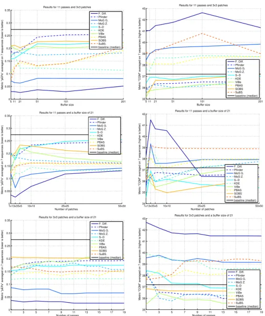
Table 1 compares the metrics for the 10 tested BGS algorithms. On average, the frame difference algorithm performs best with respect to all metrics. The best values for the other parameters are S = 21, N = 3, and γ = 11. Despite the metrics indicate our results are imperfect, Figure 1 shows that the differences between our background images and the ground-truths are barely noticeable, to the contrary of images obtained with the MED method. However, we note in Table 2 that the best BGS algorithm depends on the sequence. Figure 2 shows the performance sensitivity with respect to parameters S, N , and γ, when they vary around the optimal values given above, and compares the performance with the MED method. Despite the small size of the SBI dataset, we observed that the different metrics agree to a large extend on the ranking of the BGS algorithms for our purpose (there is a high agreement for the top 5 methods, and the frame difference is always ranked first), even if small discrepancies exist (e.g. the ranking of the MED method for the pEPs and CQM metrics).
The processing time of our method tuned with its best parameters can be easily estimated in terms of pixel throughput (the number of pixels processed per second). According to our experiments, the mean pixel throughput of a naive implementation, excluding the temporal median filter, is approximately equal to
479 × 106pixel/s for an Intel Core i7-4790K processor. Note that the most naive
implementation of a temporal median filter has an asymptotic time complexity of O(S log S), and represents an additional processing load of approximately
120 × 108pixel/s using the same processor.
4
Conclusion
In this paper, we present a simple, yet efficient, method for estimating the BG image corresponding to any video sequence taken from a fixed viewpoint. Note that the source code of our method can be downloaded at http://www.ulg. ac.be/telecom/research/sbg. The main contribution consists to embed any BGS algorithm into a generic process. For each pixel separately, this process analyses the BGS segmentation maps locally to select a subset of the frames encountered during a given number of passes. At the end of the selection process, the median is applied on the selected frames. Surprisingly, the frame difference outperforms more advanced BGS algorithms in this particular context. Results are also convincing as we obtain nearly perfect background images on the SBI dataset.
Fig. 1. The 7 video sequences of the SBI dataset (50th frame on the 1st row), the result obtained by the MED method (2nd row), our best result (F. Diff., S = 21, N × N = 3 × 3, γ = 11) (3rd row), and the corresponding ground-truth (last row). Table 1. Comparison of the BGS algorithms. The best set of parameters, as well as the averaged metrics are given for each algorithm. We selected the best sets of parameters according to the the averaged pEPs (arbitrary choice of metric).
Best parameters Averaged metrics
BGS method S N × N γ AGE pEPs pCEPs PSNR MSSSIM CQM F. Diff. 21 3 × 3 11 8.211 0.026 0.015 29.803 0.986 41.481 Pfinder 11 1 × 1 1 16.361 0.160 0.123 26.227 0.886 37.915 MoG G. 51 3 × 3 17 11.569 0.063 0.047 28.975 0.934 39.757 MoG Z. 5 50 × 50 19 13.106 0.109 0.072 25.145 0.876 37.620 S-D 11 3 × 3 1 16.029 0.141 0.111 26.619 0.881 38.324 KDE 101 1 × 1 15 11.400 0.079 0.058 27.610 0.935 39.577 ViBe 21 1 × 1 11 15.555 0.124 0.103 27.003 0.890 37.107 PBAS 11 1 × 1 9 10.406 0.057 0.039 27.030 0.947 38.550 SOBS 11 1 × 1 7 15.990 0.159 0.121 25.229 0.878 37.022 SuBS. 5 3 × 3 19 10.939 0.070 0.048 26.936 0.947 39.205
Table 2. According to the pEPs metric, the optimal BGS algorithm and set of param-eters depend on the considered video sequence.
Best parameters Metrics
Sequence BGS method S N × N γ AGE pEPs pCEPs PSNR MSSSIM CQM CaVignal F. Diff. 51 3 × 3 1 9.231 0.000 0.000 27.539 0.993 39.737 Foliage F. Diff. 201 5 × 5 19 12.018 0.015 0.000 26.019 0.992 34.113 HallAndMonitor SOBS 101 5 × 5 1 2.000 0.000 0.000 39.118 0.994 47.195 HighwayI MoG Z. 101 1 × 1 1 1.693 0.001 0.000 39.201 0.990 58.794 HighwayII MoG Z. 101 10 × 10 1 1.786 0.000 0.000 39.729 0.996 48.417 PeopleAndFoliage KDE 11 1 × 1 5 11.202 0.005 0.002 26.367 0.993 34.374 Snellen F. Diff. 11 1 × 1 5 14.858 0.056 0.047 22.426 0.982 40.001
5 11 21 51 101 201 0 0.05 0.1 0.15 0.2 0.25 0.3 0.35 Buffer size
Metric "pEPs" averaged on 7 sequences (lower is better)
Results for 11 passes and 3x3 patches F. Diff. Pfinder MoG G. MoG Z. S−D KDE ViBe PBAS SOBS SuBS. baseline (median) 5 11 21 51 101 201 35 36 37 38 39 40 41 42 43 Buffer size
Metric "CQM" averaged on 7 sequences (higher is better)
Results for 11 passes and 3x3 patches
F. Diff. Pfinder MoG G. MoG Z. S−D KDE ViBe PBAS SOBS SuBS. baseline (median) 1x13x35x5 10x10 25x25 50x50 0 0.05 0.1 0.15 0.2 0.25 0.3 0.35 Number of patches
Metric "pEPs" averaged on 7 sequences (lower is better)
Results for 11 passes and a buffer size of 21 F. Diff. Pfinder MoG G. MoG Z. S−D KDE ViBe PBAS SOBS SuBS. baseline (median) 1x13x35x5 10x10 25x25 50x50 34 35 36 37 38 39 40 41 42 Number of patches
Metric "CQM" averaged on 7 sequences (higher is better)
Results for 11 passes and a buffer size of 21
F. Diff. Pfinder MoG G. MoG Z. S−D KDE ViBe PBAS SOBS SuBS. baseline (median) 1 3 5 7 9 11 13 15 17 19 0 0.05 0.1 0.15 0.2 0.25 0.3 0.35 Number of passes
Metric "pEPs" averaged on 7 sequences (lower is better)
Results for 3x3 patches and a buffer size of 21 F. Diff. Pfinder MoG G. MoG Z. S−D KDE ViBe PBAS SOBS SuBS. baseline (median) 1 3 5 7 9 11 13 15 17 19 35 36 37 38 39 40 41 42 43 Number of passes
Metric "CQM" averaged on 7 sequences (higher is better)
Results for 3x3 patches and a buffer size of 21
F. Diff. Pfinder MoG G. MoG Z. S−D KDE ViBe PBAS SOBS SuBS. baseline (median)
Fig. 2. According to the pEPs metric averaged over the 7 sequences, the best results are obtained with F. Diff., S = 21, N × N = 3 × 3, and γ = 11. This figure shows that this is at least a local optimum as it is not possible to improve this metric by varying the parameters (left column). Moreover, we observed that our conclusion about the best set of parameters is very close to those obtained by considering other metrics (see the metric CQM in the right column). Note that the CQM metric tends to prefer an increased buffer size and a reduced number of passes. The performance of the MED method is shown as a point of comparison (baseline).
References
1. Amri, S., Barhoumi, W., Zagrouba, E.: Unsupervised background reconstruction based on iterative median blending and spatial segmentation. In: IEEE Int. Conf. Imag. Syst. and Techniques (IST). pp. 411–416. Thessaloniki, Greece (July 2010), http://dx.doi.org/10.1109/IST.2010.5548468
2. Barnich, O., Van Droogenbroeck, M.: ViBe: A universal background subtraction algorithm for video sequences. IEEE Trans. Image Process. 20(6), 1709–1724 (June 2011), http://dx.doi.org/10.1109/TIP.2010.2101613
3. Bouwmans, T.: Traditional and recent approaches in background modeling for foreground detection: An overview. Computer Science Review 11-12, 31–66 (May 2014), http://dx.doi.org/10.1016/j.cosrev.2014.04.001
4. Elgammal, A., Harwood, D., Davis, L.: Non-parametric model for background sub-traction. In: European Conf. Comput. Vision (ECCV). Lecture Notes in Comp. Science, vol. 1843, pp. 751–767. Springer, London, UK (June-July 2000)
5. Hofmann, M., Tiefenbacher, P., Rigoll, G.: Background segmentation with feed-back: The pixel-based adaptive segmenter. In: IEEE Int. Conf. Comput. Vision and Pattern Recognition Workshop (CVPRW). Providence, Rhode Island, USA (June 2012)
6. Maddalena, L., Petrosino, A.: A self-organizing approach to background subtrac-tion for visual surveillance applicasubtrac-tions. IEEE Trans. Image Process. 17(7), 1168– 1177 (July 2008)
7. Maddalena, L., Petrosino, A.: Background model initialization for static cam-eras. In: Background Modeling and Foreground Detection for Video Surveillance, chap. 3. Chapman and Hall/CRC (2014)
8. Maddalena, L., Petrosino, A.: Towards benchmarking scene background initializa-tion. CoRR abs/1506.04051 (2015), http://arxiv.org/abs/1506.04051
9. Manzanera, A., Richefeu, J.: A robust and computationally efficient motion detec-tion algorithm based on sigma-delta background estimadetec-tion. In: Indian Conference on Computer Vision, Graphics and Image Processing. pp. 46–51. Kolkata, India (Dec 2004)
10. Patwardhan, K., Sapiro, G., Bertalmio, M.: Video inpainting of occluding and occluded objects. In: IEEE Int. Conf. Image Process. (ICIP). vol. 2, pp. 69–72 (2005)
11. Sobral, A.: BGSLibrary: An OpenCV C++ background subtraction library. In: Workshop de Visao Computacional (WVC). Rio de Janeiro, Brazil (June 2013) 12. St-Charles, P.L., Bilodeau, G.A., Bergevin, R.: SuBSENSE: A universal change
de-tection method with local adaptive sensitivity. IEEE Trans. Image Process. 24(1), 359–373 (Jan 2015), http://dx.doi.org/10.1109/TIP.2014.2378053
13. Stauffer, C., Grimson, E.: Adaptive background mixture models for real-time track-ing. In: IEEE Int. Conf. Comput. Vision and Pattern Recognition (CVPR). vol. 2, pp. 246–252. Ft. Collins, USA (June 1999)
14. Van Droogenbroeck, M., Barnich, O.: Visual background extractor. World Intel-lectual Property Organization, WO 2009/007198, 36 pages (Jan 2009)
15. Wren, C., Azarbayejani, A., Darrell, T., Pentland, A.: Pfinder: Real-time tracking of the human body. IEEE Trans. Pattern Anal. Mach. Intell. 19(7), 780–785 (July 1997)
16. Zivkovic, Z.: Improved adaptive gausian mixture model for background subtrac-tion. In: IEEE Int. Conf. Pattern Recognition (ICPR). vol. 2, pp. 28–31. Cam-bridge, UK (Aug 2004)