______________________________________________
Sensitivity Analysis in the Electromagnetic
Modeling of Human Tissues
______________________________________________
By
Pouyan Ebrahimbabaie Varnosfaderani
DISSERTATION
Submitted in partial fulfillment of the requirements For the degree of Master of Science in Electrical Engineering In the Department of Electrical Engineering and Computer Science of the
University of Liège (Faculty of Applied Sciences), 2013-2014
Advisers:
Professor Christophe Geuzaine
Professor Maarten Arnst
I
ABSTRACT
The finite element method can be used to compute electromagnetic fields induced in the human body by environmental non-ionizing radiations. Such computations can be affected by uncertainty in electrical characteristics of the human body, as well as by their variability with respect to age and other physiological parameters. In this work, within a probabilistic framework, we account for the uncertainties in the electrical characteristics of the human tissues and propagate them to predictions. By restricting our attention to nonintrusive methods that can be implemented as wrappers around the finite element method (Black box), no modification of the finite element source code is required. After verifying the convergence of the method, we compute various statistical descriptors for the induced electromagnetic fields, in the brain tissues, under exposure to high frequency (microwave) and extremely low frequency (ELF) electromagnetic fields. Finally we include a sensitivity analysis of uncertainties to gain some insight into the manner in which uncertainties in the electrical characteristics of the human tissues induce uncertainties in the electromagnetic fields.
II
ACKNOWLEDGMENTS
This project would not have been possible without the support of many people. Many thanks to my advisers, Professor Christophe Geuzaine and Professor Maarten Arnst, who read my numerous revisions and helped make some sense of the confusion. Also thanks to the University of Liège. Many thanks to my parents, my brother and numerous friends, Arian, Karen, Nadege, Afshin, Abbas, Salman who endured this long process with me, always offering support and love. Finally, special thanks to Narges who changed lots of things by her kindness.
III
TABLE OF CONTENTS
PREFACE ... VI
CHAPTER 1: INTRODUCTION ...1
1.1 Computation of induced fields into the human body ...1
CHAPTER 2: LITERATURE REVIEW ...5
2.1 Uncertainty Quantification and Propagation ...5
2.1.2 Non-intrusive Methods ...6
2.1.2.1 Monte Carlo sampling method ...6
2.1.2.2 Stochastic expansion methods ...7
2.2 Stochastic Sensitivity Analysis and applications ...10
2.3 Numerical Methods for Maxwell’s Equations ...10
2.3.1 The Maxwell’s equations ...10
2.3.2 Maxwell equation in weak formulation ...11
2.3.2.1 Extremely low frequency domain ...11
2.3.2.2 Simulation in infinite spatial domains ...13
IV
TABLE OF CONTENTS
CHAPTER 3: METHODOLOGY ...16 3.1 Problem setting ...16 3.2 Characterization of uncertainties ...18 3.3 Propagation of uncertainties ...203.4 Sensitivity analysis of uncertainties ...22
CHAPTER 4: RESULTS ...24
4.1 Case A: under exposure to ELF (2D) ...24
Finite Element Method ...24
Monte Carlo Method ...26
Surrogate model ...33
Sensitivity analysis of uncertainties ...39
4.2 Case B: under exposure to RF (2D)...41
Finite Element Method ...41
Characterization of uncertainties ...45
Surrogate model ...47
Sensitivity analysis of uncertainties ...51
4.3 Interpretation of the Results ...52
CHAPTER 5: CONCLUSIONS ...54
VI
Preface
This dissertation deals with the application of spectral methods to problems of uncertainty propagation and quantification in computational electromagnetism based on finite element methods. It specially focuses on the computation of electromagnetic fields induced in the human body by environmental non-ionizing radiations. Spectral methods are probabilistic in nature, and they are consequently rooted in the rich mathematical foundation associated with probability and measure theory. However, in this dissertation, the discussion only alludes to those theoretical aspects as they are needed to set the stage for the subsequent applications. This dissertation is composed of 5 chapters. Chapter 1 discusses existing challenges in the computation of induced electromagnetic fields in the human body. This is followed by brief comments on various approaches used to deal with uncertainties. Chapter 2 focuses on numerical methods for Maxwell’s equations, and it also discusses fundamentals of uncertainly quantification, propagation and sensitivity analysis. Chapter 3 discusses so called non-intrusive methods of uncertainty propagation and their application to our problem. Chapter 4 illustrates the use of the approaches introduced in Chapter 3 by focusing on extremely low frequency (ELF) and radio frequency (RF). Chapter 5 provides a brief conclusion of the dissertation.
1
Chapter 1
Introduction
1.1 Computation of induced fields into the human body
Biological effects
People have been subject to electromagnetic (EM) radiation since the beginning of humankind. Once EM radiation came only from natural sources such as the sun and thunderstorms. Today we are subject to additional EM radiation from artificial sources. At the low end of the frequency spectrum (60 or 50 Hz) are the EM fields generated by electric power lines and small and large appliances. At the high end is nuclear radiation consisting of gamma rays and X rays. In between are the so-called radio-frequency (RF) EM waves that carry everything from AM and FM radio and television broadcasts, ham and citizen band radios, cordless and cellular phones, and personal communication devices. The term RF is layperson’s language used to describe the frequency range between a few kilohertz to several hundred gigahertz [1]. Therefore, radars for air traffic controls or for automobile speed checks, microwave ovens, computer, and other electronic products are also radiating or leaking RF EM waves, although they are not associated with radios. Very high energy electromagnetic waves, such as gamma rays or X rays, are called ionizing radiation because they ionize molecules in their paths. Uncontrolled exposure to large amounts of these waves is known to cause sickness and even death in humans [2]. The biological effects of non-ionizing RF electromagnetic waves are not well understood at this time, despite numerous of studies on the subject. There is no proof that exposure to low frequency EM fields from power -lines will cause sickness in humans. However, some studies have found a weak statistical correlation between occurrence of leukemia and length of exposure time to electric power-lines [3].
Safety limits
Most research on possible dangers from non-ionized electromagnetic radiation was researched by former Soviet Union and Eastern European Bloc countries and was quite limited until the beginning of 1970’s.Research [2]. The west also started research on the same subject, namely, the effects of EM or study of positive and negative reactions of electromagnetic fields on live organism, upon the first troubling indication. Finally, as for human exposure to RF electromagnetic fields, several organizations such as the Institute of Electrical and Electronics Engineers (IEEE) and the International Council on Non-Ionizing Radiation Protection (ICNIRP), have conducted several studies and proposed different safety limits.
IEEE safety limits
The IEEE has proposed safety limits based on more than eight years of studies by more than 100 of engineers, biophysicist, and cancer researchers. These limits are shown in the figure 1.1 [4]. At frequencies higher than 100 MHz, the human exposure limits are in terms of power density, or magnitude of the time-averaged Poynting vector. At lower frequencies, the limits are
2
expressed separately in terms of the E and H field, because each field has different biological effects.
Figure 1.1: IEEE safety limits for human exposure to RF and ELF fields
Although the IEEE standards shown in the Figure 1.1 is the accepted exposure limit at the present time, some experts recommend practicing “prudent avoidance” [1]. That is, avoid exposure to electromagnetic radiation if it can be accomplished with small investment of money or effort.
ICNIRP safety limits
The ICNIRP standard is used in most European countries and is gaining acceptance in many other countries throughout the world outside of North America. This standard provides a two-tier set of RF exposure limits. The higher tier is referred to as Occupational while the more restrictive tier is referred to as General Population. Exposure limits are given from DC to 300 GHz. Exposure limits for the magnetic field are relaxed below 100 MHz since the exposure limits at lower frequencies are based more on electro-stimulation than body heating and both induced and contact currents are related to the strength of the electric field. There are also limits for induced currents and contact currents [10]. An example of ICNIRP safety limits is shown in figure 1.2.
3
Figure 1.2: ICNIRP Exposure Limits
Computational electromagnetism
The application of computational electromagnetism (CEM) to problems involving electromagnetic fields and the human body dates back to the early 1970s. The goal was to quantify the fields penetrating in to the human body from an EM source. The techniques used in those days were mostly analytical or semi-analytical and applied to simplified object, like homogenous or layered spheres, cylinders and ellipsoids, representing the human body [5]. Later on, numerical techniques, such as the finite element methods were used with simplified models representing the tissues. In the past decade, computational hardware resource have advanced to such an extent that it is now feasible to use numerical technique to simulate and predict the inducted fields, with high degree of accuracy, in and around complex object such as a heterogeneous, anatomically realistic, human head [2]. Despite the improvements of the computer systems technology and numerous developments in techniques over the years, the results of such computations can be affected by uncertainty in electrical characteristics of the human body because of the electric properties of tissues are not precisely known and may vary depending on the individual, his/her age and other physiological parameters [11].
Problem setting
In this dissertation, first we try to use the finite element method (FEM) to compute electromagnetic fields induced in the human body by environmental non-ionizing radiations. Then within a probabilistic framework we account for the uncertainties in the electrical characteristics of the human tissues and propagate them to predictions, by restricting our attention to nonintrusive methods that can be implemented as wrappers around the finite element method (Black box). Then, we compute the probability for the electromagnetic fields to exceed thresholds defined by the international guidelines (ICNIRP), in the human tissues, under exposure to high frequency (Microwave) and extremely low frequency (ELF) electromagnetic fields. Finally we include sensitivity analysis of uncertainties to gain some insight into the manner in which uncertainties induced in the electrical characteristics of the human tissues
4
induce uncertainties in the induced fields. Despite existence of many frameworks and methods to propagate the uncertainties to predictions, here we focus on non-intrusive methods, such as stochastic expansion methods and Monte Carlo. The most attractive feature of non-intrusive methods comes with the approximations of the quantity of interest, which requires a deterministic solver only, and so needs no particular adaptation of existing codes to generate the outputs. However, the numerical cost of non-intrusive methods essentially scales with the number of deterministic model resolutions one has to perform to construct the approximation. This number of model resolutions can be large. In particular, stochastic expansion methods suffer from the curse of dimensionality (the number of model resolutions increases exponentially with the number of independent random variables in the parameterization) [7].
5
Chapter 2
Literature Review
2.1 Uncertainty Quantification and Propagation
Notation
In this dissertation, we use the following system of notation
A lowercase letter, for example, x, is a real deterministic variable.
A boldface lowercase letter, for example, x =(x1, . . . ,xm), is a real deterministic vector. An uppercase letter, for example, X, is a real random variable.
A boldface uppercase letter, for example, X=(X1, . . , Xm), is a real random vector.
An uppercase letter enclosed between square brackets, for example, [A], is a real deterministic matrix.
A boldface uppercase letter enclosed between square brackets, for example, [A], is a real random matrix.
Propagation of the uncertainties
We think of a computational model as a mapping of a set of input variables into a quantity of interest. We consider the nonlinear mapping
( ) ( )
where is the computational model, x =(x1, . . . , xm) the input variables, and the y the quantity of
the interest. Once the uncertain input variables are characterized as a random variable X with values in , the transformation of X trough the computational model provides the characterization of the quantity of interest as the random variable Y with values in such that
( ) (2.1.2)
The definition of Y as the transformation of X trough implies that the probability distribution
PY of Y is the image of the probability distribution PX of X under . For example in electromagnetic modeling of tissues, uncertain input variables could be electric conductivity or electric permittivity of the different tissues. Note that, when a vector valued quantity of interest is considered, an analysis that treats all its component simultaneously can be more informative [6].
6
2.1.2 Non-intrusive methods
The so-called non-intrusive methods rely on a set of deterministic model resolutions, corresponding to some specific values or realizations of X, to construct approximations ( ) Along this line, a deterministic simulation code can be used as a black-box (here we used the GetDP finite element solver).
Advantages
The most attractive feature of non-intrusive methods comes with the approximation of ( ), which requires a deterministic solver only, and so needs no particular adaptation of existing codes to generate the outputs. Using the computer code as a black-box also presents the advantage of making non-intrusive methods applicable to models of virtually any complexity (multi-physics, coupled problems, highly nonlinear models. . .) [7]. The numerical cost of non-intrusive methods essentially scales with the number of deterministic model resolutions one has to perform to construct the approximation. This number of model resolutions can be large. In particular, stochastic expansion methods suffer from the curse of dimensionality (the number of model resolutions increases exponentially with the number of independent random variables in the parameterization). This drawback makes non-intrusive methods computationally intensive and costly if the underlying deterministic model is expensive to solve.
2.1.2.1 Monte Carlo sampling methods
This methods is certainly quite popular, and also the simplest to implement. Monte Carlo sampling method begins by generating an ensemble of independent and identically distributed (i.i.d) samples from the probability distribution PX, written as follows:
{ }. (2.1.3)
The computational model is then used to map each sample from PX into the corresponding samples from PY that is,
( ) (2.1.4) to obtain the corresponding ensemble of i.i.d. samples from PY, written as follows:
{ } (2.1.5) Various statistical descriptors can be approximated by using methods from mathematical statics: ∑ ( ) ∑ ( ) (2.1.6)
where, is the number of samples, and are the mean and variance of the quantity of interest respectively, and are approximated values of mean and variance with respect to .
7
Effectiveness and Limitations
The Monte Carlo sampling method is most computationally efficient for problems of very high dimension, that is, for computational models with a very large number of uncertain input variables. One of the principal limitations of Monte Carlo (MC) methods concerns their convergence rate [7]. From a theoretical point of view, the law of large numbers and central limit theorem (refer to the [12]) can be used to analyze the convergence of approximations of statistical descriptors of quantity of interest such as those in (2.1.6) with respect to the number of samples. Under certain conditions, the central limit theorem ensures that accuracy improves with the square root of the number of samples [6] which is relatively low as the convergence rate. Numerous sampling methods have been proposed in order to accelerate the statistical convergence of estimators (importance sampling, variance reduction, Latin hypercube,..) but these are generally insufficient to provide accurate characterization of uncertain systems [7].
2.1.2.2 Stochastic expansion methods
Stochastic expansion methods most often involve two steps. First a surrogate model is fitted to the computational model; then, the characterization of the uncertain input variable is mapped through the surrogate model (instead of through the computational model) in to the characterization of the quantity of interest. A surrogate model is any model that mimics the relationship that a computational model establishes between the uncertain input variables and the quantity of interest and yet is computationally less expensive. Here, we focus on polynomial surrogate models.
Let elements ( ) of be referred to as multi-indices and let a (multivariate) monomial associated with a multi-index be a function from defined by . Let the number | | be referred to as the modulus of
and also the order of . Let a multivariate polynomial be a function from that maps any x to a finite sum ∑ with real coefficient . Then of order p in an m-vitiate polynomial that approximates the computational model in the PX –weighted least-square sense:
∑⌈ ⌉ ∫ | ( ) ∑⌈ ⌉ | (2.1.7)
where and, µ is the number of monomials in { | | } and { | | } collects the coefficients [6]. This procedure is pretty similar to the mathematical procedure for finding the best-fitting curve to a given set of points by minimizing the sum of the squares of the offsets (the residuals) of the points from the curve.The sum of the squares of the offsets is used instead of the offset absolute values because this allows the residuals to be treated as a continuous differentiable quantity and also the fitting technique can be easily generalized from a best-fit line to a best-fit polynomial when sums of vertical distances are used. However in this
8
case, points are distributed in the space with respect to the certain probability distribution function (PDF).
Polynomial chaos expansion
Let { | | } be a set of polynomials that span the set of all polynomials of order at most p are PX –orthonormal, that is,
∫ ( ) ( ) ⌈ ⌉ | | ( ) where PX is probability distribution of X , if and otherwise. Then polynomial chaos could be defined such that:
∑⌈ ⌉ ∫ ( ) ( ) | | (2.1.8) ( ) ∑⌈ ⌉ ( ) , (2.1.9) where the coefficients are referred to as polynomial chaos coefficients and the PX
-orthonormal polynomials as polynomial chaos. Stochastic expansion methods refer to this characterization of the quantity of interest, ∑⌈ ⌉ ( ), as a polynomial chaos expansion [6].
Nonintrusive projection methods
Despite existence of several types of implementation to obtain surrogate model (such as embedded projection or interpolatory collection method), here we describe only nonintrusive projection method. Nonintrusive projection methods approximate integrals (see equation: (2.1.8), (2.1.7)) with respect to the probability distribution PX using a quadrature rule.
Quadrature rule
A quadrature rule for integration with respect to PX is a set {( ) } of nodes and associated weight that allow the integral of any continuous, integrable function f from
with respect to PX to be approximated by a weighted sum of integrand evaluations as, ∫ ( ) ∑ ( ), (2.1.9.1)
where ∫ ( ) is referred to integration with respect to the probability distribution PX .The Gauss quadrature rule with nodes that has only positive weights and is exact for all polynomials up to order so if we set , then we can integrate exactly polynomials up to order 2P+1 [6].
First nonintrusive projection method
A first nonintrusive projection method exploits the fact that for certain “labeled” probability distribution PX, recurrence relations that can be used to produce sets { | | } of PX -orthonormal polynomials are explicitly known and can be read from tables in the literature
9
[6]. When such a set of PX-orthonormal polynomials is explicitly known in advance, the first
nonintrusive projection method provides the surrogate model as follows:
∑ ∑ ( )
| |
( ) | | (2.1.10)
That is, it provides the surrogate model by approximating the integral with respect to PX involved in the definition of the coefficients in (2.1.9) using the quadrature rule for integration with respect to PX.
Second nonintrusive projection method
A second nonintrusive projection method, which does not require a set of PX-orthonormal
polynomials to be explicitly known in advance, is obtained by approximation the integral with respect to PX involved in the definition of the objective function in (2.1.7) using the quadrature
rule for integration with respect to PX. This second nonintrusive projection method provides the
surrogate model as a solution of the following weighted least-square problem: ̃ ∑
| |
( [ ] ) [ ]( [ ] ) (2.1.11)
where is the vector, with ( ) , [M] the ( ) matrix with ( ) , and [W] the diagonal matrix with .We recall that µ is the number of monomials in { | | } and is the number of nodes in the quadrature for integration with respect to PX [6].
Notice: if [M] or [W] is rank-deficient or ill-conditioned, the use of an inadequate method may
cause a disastrous loss of numerical accuracy [6, 7]
Effectiveness
When a stochastic expansion method is used, an accurate surrogate model can usually be obtained in a computationally efficient manner if the computational model has only small or moderate number of uncertain input variables and is sufficiently smooth; once available, the propagation of uncertainties through this surrogate model usually entails virtually no overhead beyond the computational cost of its construction (low computational cost).
Limitations
Nonintrusive-projection-based implementations that use nonprobabilistic integration methods suffer from a so-called “curse-of-dimensionality” because as the number of uncertain input variables increases, nonprobabilistic integration methods lose their ability to form accurate quadrature rules with only a small number of nodes [6, 7].
10
2.2 Stochastic Sensitivity Analysis and applications
Once the characterization and propagation steps are complete, the objective of the sensitivity analysis of uncertainties is to gain some insight into the manner in which uncertainties introduced in the input variables induce uncertainties in the quantity of interest. Despite existence of several methods such as differentiation-based methods, in this section we focus only on variance-based methods.
Statistical independency
Statistically independent subsets of uncertain input variables are those between which no physical, causal relationship exists, or no logical relationship is indicated by the available information.
Significance descriptor
As the main tool for gauging the significance of a subset of uncertain input variables in inducing uncertainties in the quantity of interest, say, of the j-th subset, variance-based methods provide the following significance descriptor:
∫ (∫ ( ( ) ( ))
) (2.2.1) ( ) ∫ ( )
(2.2.2)
where denotes the random variable that collects all those components of the random variable
X that are not components of random variable [6].
Interpretation
An intuitive interpretation is obtained by recognizing ∫ ( ( ) ( ))
, as
the variance of ( ). A significance descriptor that reflects the significance of the j-th subset
of uncertain input variables in inducing uncertainties in the quantity of interest. Once all significance descriptor are available, the corresponding subsets of uncertain input variables can be arranged in order of significance.
2.3 Numerical Methods for Maxwell’s Equations
In this section we formulate the Maxwell’s equations, and discuss the finite element method to solve them. Hereafter in this section, boldface letter for example, E, is a vector.
2.3.1 The Maxwell’s equations
The fundamental theory of the electromagnetic fields is based on Maxwell’s equations. These equations govern the electromagnetic fields E, D, H and B:
11
Faraday’s law of induction: (2.3.1) Ampere-Maxwell’s law: (2.3.2) Electric Gauss’ law: (2.3.3) Magnetic Gauss’ law (2.3.4) Where
E = electric field strength (Volt per meter)
D = electric flux density (Coulombs per square meter) H = magnetic field strength (Amperes per meter)
B = magnetic flux density (Webers per square meter) or (tesla)
J = electric current density (Ampere per square meter)
= electric charge density (Coulombs per cubic meter)
Constitutive relations
Physically, the constitutive relations provide information about the environment in which electromagnetic fields occur (for example, free space, water, or plasma media)
(2.3.5) (2.3.6) (2.3.7) Where µ = magnetic permeability (H/m) = dielectric permittivity (F/m) = electric conductivity (S/m)
2.3.2 Maxwell equation in weak form
This section focuses only on the weak formulations of Radio Frequency and Extremely Low Frequency domains.
2.3.2.1 Extremely low frequency domain
In the quasi-static approximation, Maxwell’s equations (2.3.1-4) for Magnetodynamics problem are:
, , (2.3.10-a, b, c) (2.3.11) Due to the large average conductivity of tissues, the conduction currents are dominant with regard to the displacement currents and, the latter can be neglected. Besides, At ELF with such
12
conductivity ( ), the skin depth is of hundreds of meters which allows to neglect the effect of reaction field as well :
, (2.3.12) where Bs is an imposed source flux density to which the body exposed, a is magnetic vector
potential ( ) Then, using (2.3.12) and (2.3.10-a), formulation can be obtained such that:
, (2.3.13)
where, a and are magnetic vector potential ( ) and electric scalar potential (V) respectively (index s, referred to the imposed source). The computational domain ( ) can thus be restricted to the human body with an imposed boundary ( ) condition at its surface given by:
| (2.3.15) | , (2.3.14) where n is the normal vector and reference point could be any point on the surface.
The E-conform formulation
Let a be a known magnetic vector potential such that:
. (2.3.15.1) Using Faraday’s law (2.3.10-a), we can obtain (2.3.15.2):
(2.3.15.2)
where, is an unknown electric scalar potential. The weak forms of Ampere’s law (2.3.10-b), Find ( ) such that:
∫ ( ( ( ) )) ( ) ( ) , (2.3.16)
where is a test function, is the computational domain, and ( ) { ( ) ∫ ‖ ( ( ))‖ } . The time harmonic representation ( ) of the (2.3.16) is as follows:
∫ ( ( )) ( ) (2.3.17) ( ),
13
where is a test function, is the computational domain, and ( ) { ( ) ∫ ‖ ( ( ))‖ } .
2.3.2.2 Simulation in infinite spatial domains
The behavior of waves as requires the numerical treatment of boundary conditions. Several methods exist, such as Absorbing Boundary Conditions (ABC), Perfectly Matched Layer (PML), Boundary Integral Equation (BIE), etc. in this section we describe only PML.
Perfectly matched layer (PML)
A perfectly matched layer (PML) is an artificial absorbing layer for wave equations, commonly used to truncate computational regions in numerical methods to simulate problems with open boundaries.
Figure 2.3: 3D view of the PML cage.
The main idea is quite simple, wherever an X (space) derivative appears in the wave equation, it could be replace by,
( )
where is the angular frequency and is absorption function ( ).
Absorption function
Several types of absorption function exist: ( ) ( ) (Quadratic function),
( ) (Hyperbolic function),
( ) (Shifted-hyperbolic function), where, is layer thickness.
14
Action Mechanism
Wherever is positive (inside PML domain), propagating waves are attenuated because: ∫ ( )
Then
( ) ( ) ∫ ( )
Notice: should be equal to zero inside the computational domain .
2.3.2.3 Radio frequency domain
Maxwell's equations can directly give wave equation for the electric field E. Substituting Gauss' law for electricity (2.3.3), into the curl of Faraday's law of induction (2.3.1), and using the curl of the curl identity ( ) ( ) , gives the wave equation for the electric field E:
( ) (2.3.18)
where . Then we assumed, , because there is no charge density in the free space. Substituting ohm’s low ( ) in (2.3.18), gives the wave equation for the electric field such that: (2.3.19)
Time-harmonic representation ( ) of (2.3.19), is as follows:
(2.3.20)
Weak formulation
Find { ( )} such that:
∫ ( ( ))( ( )) ∫ ( )
∫ ∫ ( )
15
where , and boundary conditions have written for the figure 2.3: 1) If , (2.3.23.6)
2) If { , (2.3.23.7)
where and µ . operate such that:
( )
(2.3.23.8)
where, ( ) , ( ) , ( ) and is a damping function.
16
Chapter 3
Methodology
3.1 Problem setting
Head model
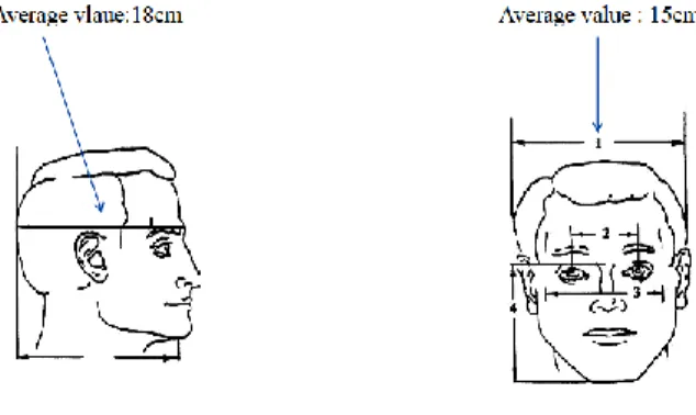
The human head is a highly complicated structure in term of material electric properties. The simplest model which can simulate the head is a box or a sphere. The sphere can either consist of a single material or comprise a central sphere of the brain white matter, which is surrounded by spherical shells of other tissues such as the brain gray matter and bone cortical also it’s possible to decrees computational cost using 2D models [3]. In this case, the head is modeled by a central ellipse of white matter which is surrounded by ellipsoidal shells of other tissues, such as the gray matter and bon cortical. You can see the realistic geometrical parameters for a normal head in the following figure,
Figure 3.1: Geometrical parameters for a normal head.
Also different anatomical regions are shown in the figure 3.2.
17
As the first step, we model the head by a central ellipse of the white matter which is surrounded by ellipsoidal shells of the gray matter and bone cortical. The geometrical parameters of each region are shown in the following figures.
Figure 3.3: 2D model of the head.
Uncertain input variables and the quantity of interest
In general, the quantity of interest should be chosen with respect to the frequency domain as well as the anatomical region of study. Regard to the ICNIRP safety limits (for the central nervous system CNS) [8], in ELF domain, the mean absolute value of the electric current density in gray matter is chosen as the quantity of interest. However, in RF domain, mean square absolute value of the electric field in gray matter is chosen as the quantity of interest. Indeed, the impacts of uncertainties in the electric characteristics of the brain tissues on the quantity of interest depend on the frequency domain. As mentioned before, in ELF domain, we assume that the relative magnetic permeability of the brain tissues is as the same as the air( ), so in such cases, only the impacts of uncertainties in the electric conductivity ( ) of tissues should be studied. However in RF domain, the impacts of uncertainties in the electric permittivity( ) should be studied as well as the impacts of uncertainties in electric conductivity of tissues.
18
3.2 Characterization of uncertainties
Probability Distribution Function (PDF)
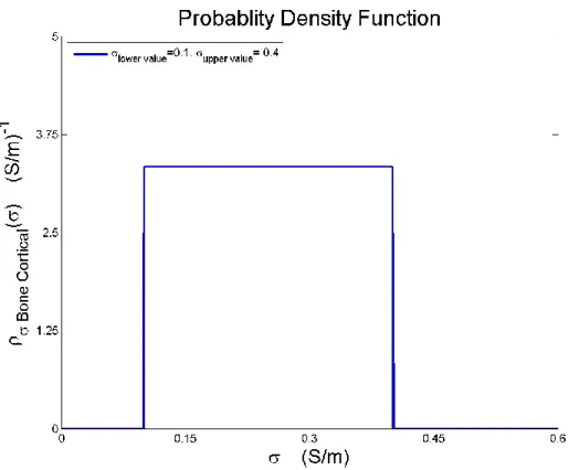
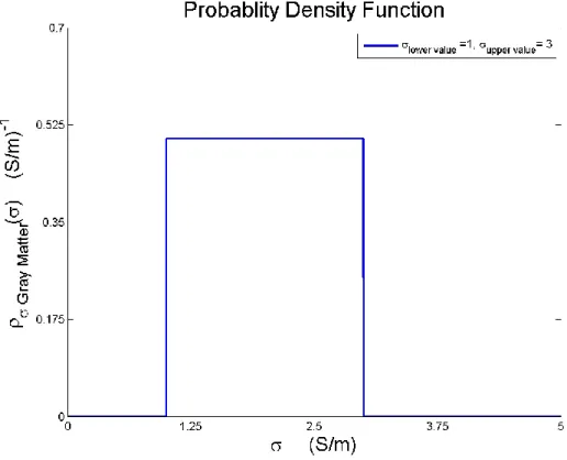
As the second step, we focus on finding the PDF of uncertain input variables. We assumed the electric conductivities of different tissues as the uncertain input variables. According to the principle of maximum entropy, if nothing is known about a distribution except that it belongs to a certain class, then the distribution with the largest entropy should be chosen as the default. In ELF domain, for electric conductivities, only two (or even only one) values per frequency point could be found among different references [9]. So, the uniform distribution is the best choice among all other labeled probability distributions. Because of The uniform distribution on the interval [a,b] is the maximum entropy distribution among all continuous distributions which are supported in the interval [a,b] (which means that the probability density is 0 outside of the interval). The probability distribution functions of electric conductivity in each anatomical region are shown in the following figures.
19 Figure 3.5: PDF of the in 50 Hz. Figure 3.6: PDF of the in 50 Hz.
20
3.3 Propagation of uncertainties
Monte CarloThe Monte Carlo sampling method begins by generating an ensemble of independent and identically distributed samples from the probability distribution . In this problem, three cases could be imagined. If electric conductivity only in one region was uncertain or electric conductivities were uncertain in two or even three different regions, such cases called 1D, 2D and 3D respectively. The computational model is then used to map each samples from its probability distribution into the corresponding sample form . For example, we may characterize a 3D case as follows:
Figure 3.7: FEM as a mapping of into the .
{( ) } , (3.3.1) ( ) . (3.3.2)
Now, it’s possible to obtain, corresponding ensemble of i.i.d samples from , written as follows:
{ } . (3.3.3)
Once these i.i.d samples from are available, various statistical descriptors can be approximated using methods from mathematical statistics. For example, the mean and variance (if they exist) can be approximated as:
∑ , ( ) ∑ ( ) . (3.3.4) This implementation is nonintrusive because it requires only the repeated solution of the computational model for different values assigned to its uncertain input variables.
21
Polynomial based surrogate model
Regard to relations which explained in detail in section 2.1.4, polynomial based surrogate models for each case (1D, 2D or 3D) could be obtained using second non-intrusive projection based method. This section discusses about 3D cases:
Figure 3.8: Surrogate model as a mapping of into the .
( ) ( ) ∑ ∑ ∑ , (3.3.5)
To find we used the second non-intrusive projection method (explained in page 9) also to prevent ill-conditioning in matrix [M] (for higher order of P), uncertain input variables should be normalized for constructing of the surrogate model. So the equation 3.3.5 should be written as follows: ( ) ( ) ∑ ∑ ∑ ( ) ( ) ( ) (3.3.6)
where, ( ) is the mean value and ( ) means standard deviation (STD). Some statistical
descriptors could be obtained directly from the surrogate model. Let {( ( ) ( )) } ,
{( ( ) ( )) } and {(
22
and weights in each dimension, then the mean and variance of the inducted current density in the gray matter could be obtained by the following relations (integration of surrogate polynomial with respect to the PDF):
∑ ∑ ∑ ( ( ) ( ) ( )) ( ) ( ) ( ) ( )
( ) ∑ ∑ ∑( (
( )
( ) ( )) )
( ) ( ) ( ) ( )
These values converge to , by increasing the order of polynomial (P).
3.4 Sensitivity analysis of uncertainties
Intuitive method
Once the characterization and propagation steps are complete, then the next step would be sensitivity analysis. The objective of the sensitivity analysis of uncertainties is to gain some insight into the manner in which uncertainties introduced in the input variables induce uncertainty in the quantity of interest. This section focuses on intuitive method, based on comparison of uncertainty percentages. Intuitive method includes the following steps:
Step 1: Compute the uncertainty percentages, for all of the uncertain input variables using the following formula,
( ) ( )
Step 2: Set all of the uncertain input variables except one (for example: ) to their mean values
then using MC to compute uncertainty percentage of output.
Figure 3.9: FEM as a mapping of into the
Step 3: Repeat step 2, for the rest of the uncertain input variables. Step 4: Interpretation of the results.
23
Variance based method
Regard to the relations (2.2.1) and (2.2.2) which described in detail in the chapter 2, in 3D cases, significance descriptor or Sobol coefficient of the gray matter ( ) obtained using the following relations (same methods for and ):
( ) ( ) ∬ (∫ ( ( ) ( )) ( ) ) ( ) ( ) , (3.3.11) ( ) ∫ ( ) ( ) (3.3.12) ∬ (∫ ( ( ) ( )) ( ) ) ( ) ( ) , (3.3.13) ( ) ∫ ( ) ( ) (3.3.14) ∬ (∫ ( ( ) ( )) ( ) ) ( ) ( ) , (3.3.15) ( ) ∫ ( ) ( ) (3.3.16)
As mentioned before, once all of the descriptors are available, the corresponding uncertain input variables can be arranged in order of significance. The higher means more significance of the uncertain input variable of in inducing uncertainties in the inducted current density in the gray matter.
24
CHAPTER 4
RESULTS
4.1 Case A: under exposure to ELF (2D)
Finite Element method
We assumed that, the magnetic field and frequency are equal to, 4 (µT) and 50 (Hz) respectively, also in this section (Finite Element Method), we set to the mean values ( =0.007 (S/m), =0.26 (S/m) , = 0.16 (S/m) ). The results are shown in the following figures (where the magnetic field is perpendicular to the surface).
Imaginary part of electric current density ( ) , where the real part is equal to zero.
25
Imaginary part of electric field ( ) , where the real part is equal to zero.
Figure 4.2
Equipotential lines ( ) , where the real part is equal to zero. Figure 4.3
26
As you can see, in the figure 4.1, has the higher value in the gray matter rather the other anatomical regions, due to the higher value of .
Monte Carlo method
Case 1D:
Let , be the only uncertain input variables (see page 21) using MC, we obtained the
following results:
Figure 4.4: FEM as a mapping of into the .
27
Figure 4.6: Convergence study of rather number of samples (MC-1D).
Case 2D:
Three different situations could be imagined: Case A:
Figure 4.7: FEM as a mapping of into the .
Case B:
Figure 4.8: FEM as a mapping of into the .
Case C:
28
Case A:
(100 random realizations) Figure 4.10
29
Case B:
(100 random realizations) Figure 4.12
30
Case C:
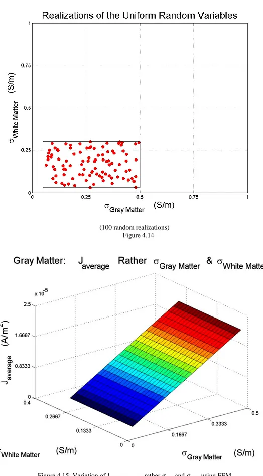
(100 random realizations) Figure 4.14
31 Case 3D
:
Let , and be uncertain:
Figure 4.16: FEM as a mapping of into the .
(100 random realizations) Figure 4.17
32
Figure 4.18: Convergence study of rather number of samples (MC-3D).
33
Figure 4.20: PDF convergence study (MC-3D).
Surrogate Model
Case 1D:
Let , be the only uncertain input variables (see page 21) using surrogate model, we
obtained the following results:
GetDp is replaced by Surrogate model. Figure 4.21
34
Figure 4.21: FEM and Surrogate model (1D).
Figure 4.22:
35
Figure 4.22: ( ) .
Case 2D:
Case A: Let be uncertain (here we explained only (Case A), other cases could be obtained using the same method).
36
Figure 4.24: Variation of rather and using FEM and Surrogate model.
Figure 4.25: .
37
Figure 4.26: ( ) .
Case 3D:
Let and be uncertain, using the following algorithm we can compare results. Beside these it’s possible to obtain statistical descriptors from the polynomial directly.
38
Figure 4.28: Mean convergence study for the Case 3D using surrogate model and FEM.
39
Figure 4.30:
Sensitivity analysis of uncertainties Intuitive method:
Step1: Compute the uncertainty percentages, for all of the uncertain input variables
Uncertain Input Variable STD (S/m) Mean (S/m)
( )
40
Step 2 &3:
Uncertain Input Variable STD (A/m2) Mean (A/m2)
( )
Uncertain Constant Constant Constant Uncertain Constant Constant Constant Uncertain
Table 4.2:uncertainty percentages of in different situations (see: section 3.4).
Step4:
As you can see, one percent uncertainty in led to, about once percent uncertainty in . However, effects of uncertainties in and could be ignored.
Variance based method:
Regard to the section 3.4, relations (3.3.10-12), we obtained the significance descriptors as the follows:
( ) ( ) , ( ) .
41
4.2 Case B: under exposure to RF (2D)
Finite Element Method
Regard to section 2.3.4, positions in the PML cage, head, dipole and their geometrical parameters have shown in the following figure:
Figure 4.32: Head and the PML cage
We assumed that, the frequency is equal to 1.8 GHz also by fixing and to their mean values, we obtained the following results (by restricting our attention to the head).
42
Imaginary part of electric current density ( ) . Figure 4.33
Real part of electric current density ( ) . Figure 4.34
43
Real part of the magnetic field ( ) , Figure 4.36
Imaginary part of the magnetic field ( ) . Figure 4.37
44
Real part of the magnetic field ( ) . (Second view)
Figure 4.38
Norm of the electric field | | ( ). Figure 4.39
45
Characterization of uncertainties
As the first step we should define, PDFs of the uncertain input variables .we assumed the electric conductivities of different tissues as the uncertain input variables. According to the principle of maximum entropy, if nothing is known about a distribution except that it belongs to a certain class, then the distribution with the largest entropy should be chosen as the default. Despite existence of the several values for electric conductivity on 1 GHz, on 1.8 GHz, only one value could be found among different references. So, the uniform distribution is the best choice among all other labeled probability distributions. Because of The uniform distribution on the interval [a,b] is the maximum entropy distribution among all continuous distributions which are supported in the interval [a,b] (which means that the probability density is 0 outside of the interval). The probability distribution functions of electric conductivity in each anatomical region are shown in the following figures.
46
Figure 4.41: PDF of the in 1.8 GHz.
47
Surrogate Model
Case 2D:
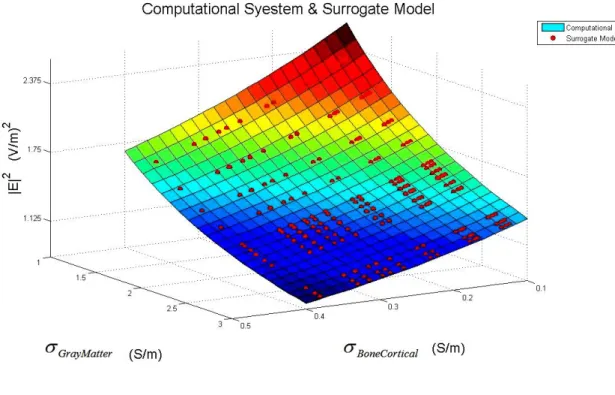
Let and be uncertain, using the following algorithm we can compare results. Beside these it’s possible to obtain statistical descriptors from the polynomial directly.
Figure 4.43: Comparison between surrogate model and FEM (Case 2D).
48
Figure 4.45: | | .
49 Case 3D:
Let and be uncertain, using the following algorithm we can compare results. Beside these it’s possible to obtain statistical descriptors from the polynomial directly.
Figure 4.45: Comparison between surrogate model and FEM (Case 3D).
50
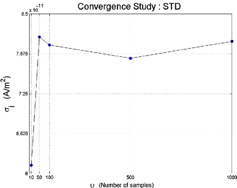
Figure 4.47: STD convergence study for the Case 3D, using surrogate model and FEM.
51
Sensitivity Analysis
Variance based method:
Regard to the section 3.4, relations (3.3.10-12), we obtained the significance descriptors as the follows:
( ) , ( ) , ( ) ,
| | ( ) .
52
4.3 Interpretation of the results
Extremely Low Frequency Domain (ELF):
Sensitivity analysis of uncertainties
As the last step, we carried out a sensitivity analysis of uncertainties, to gain insight into the manner in which uncertainties in the electric conductivities, induce uncertainty in electric current density in the gray matter. Using the variance based method, we obtained the following approximations of the significance descriptors for P=2 and =3:
Uncertain Input Variable
(A/m
2)
2
(
)
Table 4.3: Uncertain input variables with their significance descriptors
Thus the uncertainties in the electric conductivity of the gray matter are much more significant than those in the bone cortical or white matter in inducing uncertainties in the electric current density in the gray matter.
Numerical convergence study
We conducted a numerical convergence study (for all of the three cases) to examine the impact that the values assigned to P and on the results. Specially, we repeated the construction of the surrogate model and the approximation of statistical descriptors for several values of P and setting . We observed that the results presented previously for P=1 and have converged reasonably with respect to the order P of the surrogate model and the parameter that controls the number of nodes in quadrature for integration with respect to the PDFs.
53 Radio Frequency Domain (RF):
Sensitivity analysis of uncertainties
As the last step, we carried out a sensitivity analysis of uncertainties, to gain insight into the manner in which uncertainties in the electric conductivities, induce uncertainty in square norm of the inducted electric field in the gray matter. Using the variance based method, we obtained the following approximations of the significance descriptors for P=2 and =3:
Uncertain Input Variable
(V/m)
4
(
| |)
Table 4.3: Uncertain input variables with their significance descriptors
Thus the uncertainties in the electric conductivity of the gray matter and bone cortical are respectively much more significant than those in the white matter in inducing uncertainties in the square norm of the electrical field in the gray matter.
Numerical convergence study
We conducted a numerical convergence study (for all of the three cases) to examine the impact that the values assigned to P and on the results. Specially, we repeated the construction of the surrogate model and the approximation of statistical descriptors for several values of P and setting . We observed that the results presented previously for P=2 and have converged reasonably with respect to the order P of the surrogate model and the parameter that controls the number of nodes in quadrature for integration with respect to the PDFs.
54
Chapter 5
Conclusions
Computational efficiency of the polynomial surrogate model
In this dissertation, we covered sensitivity analysis in the electromagnetic modeling of the human head in its entirety. Both high and low frequency cases are included. In particular, in regard to the ICNIRP safety limits (for the central nervous system CNS), we focused on quantifying induced uncertainties in the electric current density and square norm of the electric field in the gray matter using Monte Carlo and stochastic expansion methods. These non-intrusive methods are implemented as wrappers around the finite element method (using GetDP as the finite element solver). We observed that, in this particular problem, despite the effectiveness of the Monte Carlo method (for computational models with a very large number of uncertain input variables), the polynomial surrogate model is much more computationally efficient than the Monte Carlo method due to its low computational cost and other advantages. We obtained statistical descriptors such as the mean and the variance directly from the surrogate model using the Gauss quadrature rule.
Sensitivity analysis of uncertainties
Finally, we carried out a sensitivity analysis of uncertainties. Despite the existence of several types of sensitivity analysis of uncertainties, such as methods involving scatter plots and regression, correlation, and elementary effects and differentiation based methods, in this dissertation we focused on intuitive and variance-based methods. We observed that, in the ELF domain, uncertainties in the electric conductivity of the gray matter are much more significant than those in the bone cortical or white matter in inducing uncertainties in the electric current density in the gray matter. In the RF domain, uncertainties in the electric conductivity of the gray matter and bone cortical regions are much more significant than those in the white matter in inducing uncertainties in the square norm of the electric field in the gray matter.
Challenges
Note that we used a quite pessimistic statistical law for the conductivities (uncertain input variables) due to the limited number of available samples. For example, In ELF domain, for the electric conductivities, only two values, or sometimes even only a single value per frequency point could be found in the consulted references. We chose the uniform probability distribution. Indeed, the uniform distribution on the interval [a,b] is the maximum entropy distribution among all continuous distributions which are supported in the interval [a,b] (which means that the probability density is 0 outside of the interval). Note that the presented stochastic expansion method is only effective for small or moderate number of uncertain input variables. With many uncertain parameters the proposed approach could be accelerated using advanced stochastic expansion methods. Much recent research has investigated how the computational cost of
55
stochastic expansion methods can be reduced, as well as how their range of applicability can be extended to problems of higher and higher dimensions and to computational models that lack smoothness. In particular, alternative (not necessarily polynomial) basis function and alternative formulations of the construction of the surrogate model are being investigated.
56
References
1
. Liang Chi Shang, J. A. (1995). Applied Electromagnetism (3rd Edition). Boston: PWS PUBLISHING COMPANY.
2.
P.Stavroulakis. (2003). Biological Effects of Electromagnetic fields. Berlin: Springer3.
P.Thomas. (1993). Power Struggle. Harvard Health Letter, VoL. 18,no .9 , P 14.
Fischetti, M. (June 1993). The Cellular Phone Scare. IEEE Spectrum , P. 43.5.
H.Massoudi, C. D. (1997). Long-wavelength electromagnetic power absorption in elipsoidal models of man and animals, Vol 25. IEEE , P 47-52.6.
Maarten Arnst, J.-P. P. (2013). AN OVERVIEW OF NONINTRUSIVECHARACTERIZATION,PROPAGATION,AND SENSITIVITY ANALYSIS OF UNCERTAINTIES IN COMPUTATIONAL MECHANICS. International Journal for
Uncertainty Quantification .
7.
O.P. Le Maître, O. K. (2010). Spectral Methods for Uncertainty Quantification withapplication to computational fluid dynamics. New York: Springer.