Single point incremental forming simulation with adaptive remeshing technique using solid-shell elements

Single Point Incremental Forming Simulation with Adaptive

Remeshing Technique using Solid-Shell element

J.I.V. Sena

, C. Lequesne

, L. Duchene

, A.M. Habraken

, R.A.F. Valente

, R.J.

Alves de Sousa

a_{GRIDS Research Group, TEMA Research Unity, Department of Mechanical Engineering, University of} Aveiro, 3810-193 Aveiro, Portugal, sena.ilidio@ua.pt, robertt@ua.pt, rsousa@ua.pt

b_{Université de Liège, ArGEnCo Department, MS²Fdivision, Chemin des Chevreuils 1, Liège, 4000,} Belgium, cedric.lesquesne@gmail.com, l.duchene@ulg.ac.be, anne.habraken@ulg.ac.be

ABSTRACT

Single Point Incremental Forming (SPIF) is a dieless manufacturing process in which a sheet is deformed by using a tool with a spherical tip. This dieless feature makes the process appropriate for rapid-prototyping and allows for an innovative possibility to reduce overall costs for small batches, since the process can be performed in a rapid and economic way without expensive tooling. As a consequence, research interest related to SPIF process has been growing over the last years.

Numerical simulation of SPIF process can be very demanding and time consuming, mainly due to the the high non-linearity and constantly changing contact conditions between the tool and the sheet surface, as well as the nonlinear material behavior combined with non-monotonic strain paths. To reduce the simulation time, in the present work an adaptive remeshing technique is proposed being implemented in the in-house implicit finite element code LAGAMINE. This remeshing technique automatically refines only a portion of the sheet mesh at the tool’s vicinity, therefore following the tool’s motion. As a result, uniformly refined meshes required for accuracy purposes are avoided and consequently, the total CPU time can be drastically reduced.

In this work, the proposed automatic refinement technique is applied developed within a Reduced Enhanced Solid-Shell (RESS) framework to further improve numerical efficiency. Finally, validations by means of benchmarks are carried out, with comparisons against experimental results.

Keywords: single point incremental forming; adaptive remeshing method; solid-shell finite element

formulations; implicit analysis, sheet metal forming

† _{Corresponding author}

J.I.V. Sena

Department of Mechanical Engineering, University of Aveiro, 3810-193 Aveiro, Portugal Phone: +351234378150, Fax: +351234370953, Email: sena.ilidio@ua.pt

1. Introduction

Sheet metal forming is a widely used manufacturing process, being nowadays well-developed. The final products have good quality, are geometrically accurate and it allows the production of parts ready to be used. Additionally, the process is used for large batches which amortize the cost of the tools, producing large quantities of components during a short time interval. However, the possibility to use conventional stamping processes to build low production’s batches or personalized prototypes can be expensive.

In R&D processes, prototype manufacturing is an important step in product development. Consequently, it is important to shorten the product’s life-cycle and costs in its initial development. As a result, Incremental Sheet Forming (ISF) appears as a new possibility to decrease the costs in small volume production (Jeswiet et al., 2005). It introduces the use of metallic sheet for small batches production in an economic way without the need of expensive tooling or dedicated tools. In fact, the study and development of this process has been growing over the last years. An extra innovative advantage of ISF technology is the possibility to produce parts in polymeric sheet, which is difficult to achieve with traditional forming methods.

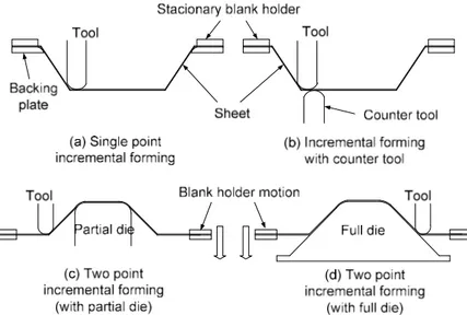
The ISF process evolved since the 90’s, and new variants were developed and patented (Emmens et al., 2010). In the literature, ISF processes are referenced as belonging to a group called asymmetric incremental sheet forming (AISF). The AISF variants can include four different configurations techniques (Jeswiet et al., 2005), as shown in Figure 1.

Figure 1 – Asymmetric incremental sheet forming variants.

The main common aspect in these variants is the use of a spherical forming tool in constant contact with the workpiece. The sheet is also clamped at its edges using a blank-holder. During forming, the tool travels along the workpiece, following a specific trajectory chosen by the user.

In the present work, particular attention is devoted to the Single Point Incremental Forming (SPIF) variant (Figure 1.a). SPIF can be considered as the real dieless forming technology, as envisioned by Leszak (Leszak, 1967). Within the AISF process group classification, the SPIF method is also called “negative forming” (Park and Kim, 2003), with its application being a breakpoint with traditional forming processes.

The classic press-stamping process deforms the sheet metal in only one step (can also be in multiple steps). The sheet is forced by a punch against a mould, stretching the blank to the desired shape, while the edges are restrained by a blank holder but also allowing some sliding. In the SPIF process, on the other hand, the sheet metal is gradually deformed by a localized force. The tool is guided through a numerical control system, which defines the tool path according to the final shape. The pre-programmed contour combines the continuous contact of the tool along the sheet surface with successive small vertical increments. After each vertical increment, a contour in the next horizontal plane starts, with the final component being formed layer by layer. The backing plate shown in Figure 1.a is needed to decrease springback effects during forming. The springback phenomenon can also be avoided using a

compensatory algorithm (Allwood et al., 2010). In any case, the opposite surface does not contact with any die or support.

Experimental and numerical research works, came to the conclusion that classical theories applied to conventional stamping processes were not suitable for SPIF. Particularly, there are evidences that point to an apparent increased formability and different deformation mechanisms (Eyckens et al., 2009) in SPIF.

The main goals of experimental developments in the literature include process optimization and the understanding on how its physical characteristics can influence forming. A number of authors experimentally studied the final product in order to analyse the influence of several parameters involved in the SPIF process. The following forming parameters were discovered to be important in SPIF process: the geometry of the forming tool, the sheet material, the sheet thickness, the tool path, the increment size, the forming speeds (rotation and relative motion) and lubrication (Ambrogio et al., 2011; Durante et al., 2009; Cerro et al., 2006; Kim et al., 2002; Kopac and Kampus, 2005).

Due to the vast number of new topics, many works have been carried out dealing with particular aspects of the process. From the numerical simulation standpoint, the SPIF process represents a particular challenge concerning computation time, which tends to be higher than those of conventional processes, both for implicit or explicit analysis. Previous results in the literature show that numerical simulation needs a compromise between accuracy and CPU efficiency related to the temporal integration scheme, material law, finite element formulation and mesh size (Lequesne et al., 2008; Bouffioux et al. 2008; Henrard, 2008; Eychens et al., 2009; Hadoush and van den Boogard, 2008 and 2009; Aerens et al., 2010; Sena et al. 2011, Arfa et al., 2012).

The current paper presents the numerical validation of adaptive remeshing procedure using a solid-shell finite element formulation. The paper is divided into seven main topics: i) an introduction; ii) a brief state-of-the-art about numerical simulation developments; iii) the description of the adaptive remeshing method developed; iv) the formulation of RESS finite element used in numerical simulation of SPIF; v) a sensitivity analysis of the adaptive remeshing parameters; vi) the numerical simulation results for an incrementally formed conical shape, and vii) the final considerations.

2. Numerical simulation of SPIF: A review

Single point incremental forming (SPIF) can be an interesting option in the prototyping and small batches production, as previously outlined. The literature review presented in the following focus with more emphasis the research work about numerical simulation developments, with the aim to provide a better understanding on the process and its peculiarities.

Many issues appear when simulating SPIF process resorting to the Finite Element Method (FEM). As always, a compromise between accuracy and CPU efficiency is necessary. Accuracy from the numerical simulation’s results, specially related to the prediction of the forming forces, is important and contributes to the protection of the tool and the machinery used in the process.

The adopted temporal integration scheme, the finite element formulation and mesh refinement procedure are the main topics in present work. Below, it is presented a brief summary of numerical studies about different aspects of the process, as found in the literature.

FEM is an approximation technique which computes the solution of algebraic equation systems, based on equilibrium equations, which depend of the problem type and can be static or dynamic. The integration of these equations over time can be based on two different integration schemes: explicit or implicit. Both solution procedures are commonly available in commercial FEM codes, having been investigated for SPIF process simulation in the literature.

Bambach and Hirt (2007) have carried out FEM analyses about SPIF processes with ABAQUS/Explicit and ABAQUS/Standard (ABAQUS, 2005), for optimizing the tool path. Those authors compared the values of sheet thickness and geometry accuracy against the experimental results along a radial section of a conical shape. The blank was modelled with shell finite elements and the friction coefficient was set to zero in the Finite Element model. As a result, the authors concluded that an explicit scheme using scaling time step of 10-4_{s was a suitable choice. When compared to a mass scaling} procedure (with a time step of 10-5_{s), obviously the results didn’t deteriorate considerably, however the} calculation time increases from 30 minutes to more than three hours. A direct comparison of the thickness provided using the explicit and implicit analyses demonstrates that the maximum difference between both schemes occurred when the vertical pitch is performed. Due to the high kinetic energy transmitted through the tool during the sudden change from the in-plane movement to the vertical pitch (Bambach

and Hirt, 2007). The obtained force also has a deviation when the vertical displacement is performed. To avoid the vertical pitch influence, the spiral tool path was tested and the tool forces obtained in the implicit and explicit scheme were in good agreement.

Yamashita et al. (2008) have used a dynamic explicit finite element code LS-DYNA to perform a quadrangular pyramid with variations in its height. Several types of tool paths were tested in order to find the effect on the deformation behaviour. The thickness strain distribution and the force acting during the tool travel were evaluated. The effect of the density of the sheet material and the travelling speed of the tool are pre-examined and optimized to determine the computational condition to use in the simulation in LS-DYNA, for reducing the computational time. It was concluded that numerical simulation using explicit scheme might be used for the tool path optimization of the SPIF process.

Sena et al. (2011) have validated the results coming from numerical simulations of SPIF process using the reduced enhanced solid-shell (RESS) formulation (Sousa et al., 2007), and comparing it with solid finite elements available in ABAQUS software (ABAQUS, 2005). In this preliminary work, isotropic hardening and implicit analysis were considered. The results from numerical simulations were also compared to those obtained with the experiments. The experimental results were used as reference to assess the effectiveness of several finite element formulations, including the RESS formulation and a set of solid (eight node, 3D) finite element options, namely: C3D8 (full integration), C3D8R (full reduced integration) and C3D8I (full integration with incompatible deformation modes) available in ABAQUS. The main differences between ABAQUS solid elements and the RESS element is the possibility to vary the number of integration points through the sheet thickness, in the latter formulation. For ABAQUS solid elements, the number of layers through the thickness direction must be increased in order to have more than one (C3D8R) or two (C3D8/C3D8I) integration points per layer in this direction. With the RESS formulation, on the other hand, the number of integration points can be unlimited increased within a single layer.

Concerning the role of the finite elements adopted here, it was concluded that reduced and selective reduced integrated solid elements have significant error levels when simulating SPIF processes (Sena et al., 2011). The addition of Enhanced Assumed Strain (EAS) modes, as appearing in RESS formulation, was shown to improve the overall quality of results. A plausible explanation is the bending-dominated deformation mechanisms that appear during the forming process, usually better described using enhanced strain-based formulations. RESS finite element, using enhanced deformations, provides better or at least comparable results with conventional solid finite elements from commercial packages. However, the use of this formulation can help decrease the computational cost, given the special integration scheme employed, and that is the reason to also use this formulation in the present work.

Henrard (2008) have developed a strategy to perform SPIF simulations with dynamic explicit integration time scheme with an in-house code called LAGAMINE (Cescotto and Grober, 1985). The simulations were performed using a line test benchmark, and the mesh model was built with the COQJ4 shell element (Jetteur and Cescotto, 1991; Li, 1995). Initially, the line-test simulation was run without mass scaling and using different diagonal mass matrices (Henrard, 2008). However, the results were not satisfactory due to poor shape accuracy when compared with implicit strategies. The mass-scaling value increases the largest stable time step and speed up the simulation. The computation time with mass-scaling factor of 104 _{is around 50% of the computation time of the implicit scheme. However, a} mass-scaling factor of 103 _{guaranties the stability but the CPU time does not decrease, and the use of dynamic} explicit strategy introduces inertia terms into the equilibrium equations. The choice of the mass-scaling factor affects the compromise between accuracy and the computation time. The explicit strategy was therefore shown to be more unstable than the implicit approach, with mesh sensitivity higher than with an implicit scheme.

Lequesne et al. (2008) have implicitly modelled the SPIF process using LAGAMINE. In order to decrease the simulation time of SPIF simulation combined with an implicit integration scheme, a new method using adaptive remeshing procedure was developed. The sheet mesh was modelled with 4-node shell element implemented in the code, called COQJ4. The contact surface uses the same nodes connectivity of the shell finite element combined with classical penalty method (Habraken and Cescotto, 1998). The spherical tool was modelled as a rigid body. Once this paper deal with the extension of this method from shell to solid-shell elements, its detailed description will be given in the next section, Section 3. The validation of adaptive remeshing in SPIF process for shell elements was performed using a line test simulation from the work of Boufioux et al. (2008).

Hadoush and van den Boogaard (2008) have proposed an implementation of a mesh refinement/derefinement (RD) approach to reduce the computing time of SPIF process simulation. The RD approach consists in a refined mesh in the vicinity of the tool since there is a small contact area between the tool and the sheet metal, while the rest of the sheet can have a coarse mesh. During the process simulation, the mesh connectivity is continuously changing, because of the tool motion. This

approach is implemented in an in-house implicit FE package. The finite element type used is a triangular shell element and each coarse element is divided in four new refined equal elements when it is in the tool neighborhood. The main goal of this approach is to keep the number of elements as low as possible during the simulation. In the numerical simulation it is used a pyramid with 45º of wall as the analysis test. The state variables, when the new refined elements are generated, are transferred from the old coarse element to the new smaller elements. To conclude, the RD approach reduces the computing time for the reference model approximately 50%. The achieved equivalent plastic strain with this approach showed a good agreement with the reference model.

The main differences between the remeshing procedure which will be described in Section 3 and the one proposed by Hadoush and van den Boogaard (2008) are the finite elements type used and the refinement/derefinement criterion. In this last approach, the refinement criterion is performed if the geometrical error exceeds an indicator value. It measures the variation of the geometry within the blank. This variation is based on a set of tangent axes determined for each element. The variation of these sets of tangents from each element to its neighbourhood elements indicates the geometry variation. A nodal averaging technique is used to quantify this variation. The derefinement occurs if the variation within the group of refined elements decrease and it is less than the user input value. Consequently, the coarse element takes the place of the refined elements.

From this brief literature review, the authors that use commercial codes have claimed that the explicit scheme is the most appropriate, instead of implicit scheme. The authors that use the implicit scheme achieved equivalent results and it is ensured that the results have converged correctly. However, a refinement strategy solution was adopted to reduce the computation time using the implicit scheme. These features are not available in common commercial FEM code. In this work, a special focus will be given to the adaptive remeshing method chosen, the finite element formulation implemented and the numerical integration schemes. To keep the referred focus, implicit analysis is used to perform the numerical simulations. It is worth noting that no previous work has been carried out using remeshing strategies with solid elements, which makes this work innovative. Solid and solid-shell elements are important to provide generality as using full 3D constitutive modelling and direct thickness measurement.

3. Adaptive remeshing method

This section introduces and describes the adaptive remeshing method implemented in the finite element in-house code LAGAMINE, developed at the University of Liège (Lequesne et al., 2008). This remeshing method is currently available for two different types of finite elements: shell finite element and eight nodes solid-shell finite element, specifically the RESS finite element.

In SPIF, the blank surface where high deformations occur is always close to the current tool location. In this technique only a portion of the sheet mesh is dynamically refined at the tool vicinity and following its motion. Doing so, the requirement of initially refined meshes is avoided and consequently, the global CPU time can be reduced.

Figure 2 – Adaptive remeshing procedure.

The adopted remeshing criterion is based on the shortest distance between the centre of the spherical tool and the nodes of the contact finite element. The size of the tool vicinity is defined by the user through the expression:

(

+

) ,

2 2 2

D

≤

α L

R

The coarse element respecting the criterion is deactivated and become a “cell” (storage name for new elements) which contains all information about the new smaller elements. Each coarse element is divided into a fixed number of new smaller elements. The generation of all new nodes in a cell is located between two old nodes, A and B.

A 1

B 2

p n

: Old Nodes : New Nodes Figure 3 – Generation of new nodes.

Its current positions, last step position and initial position are computed using the following interpolation:

,

p

p

= 1-

+

n+1

n +1

























q

q

q

where n is the number of new nodes between A and B, p is the new node number, qp, qA and qB are

respectively the degrees of freedomof node p. The local coordinate,

ξ

2p

ξ =

- 1 .

n +1

The sequential procedure to geometrically divide the coarse element starts with the contact element partition. Subsequently, the partition information is transferred from the contact element to split the solid-shell element. The information transferred between contact element and solid-solid-shell element is performed by using pointers (memory allocation).

The transference of stresses and state variables from the coarse elements to the new elements is performed using an interpolation method. The interpolation method is based in a weighted-average formula from the work of Habraken, (1989). The transference is performed from the integration points of the coarse finite elements in the vicinity of the new integration point which belong to the new elements generated.

During the simulation, selected cells of refined elements are removed. This remeshing method creates selected nodes that are incompatible with the non-refined finite element with common edge. As this does not take into account any transition zone between coarse and fine elements, there are three types of nodes: old nodes, free new nodes and constrained new nodes. The nodes which belong to a cell edge with common edge with a removed cell or with a coarse element non-refined become constrained nodes (Figure 4) or also mentioned as slaves nodes. The constrained nodes are used to allow the structural compatibility of the mesh. The degrees of freedom and positions of the constrained nodes on a “cell” edge depends on the two old master-nodes, which are extremities of this edge. The new slave-nodes can have a different position from the initial relative position between the two old nodes (masters) because they were free before. Doing so, new relative positions are computed based in the intersection of the segment between the two master nodes.

Figure 4 – Constrained nodes generation during the adaptive remeshing method.

The constrained nodes must remain at the same relative positions between two old master-nodes and the elements where the nodes belong have a new shape. Consequently, the global list of degrees of freedom (DOF) is modified. The DOF of the slave nodes are replaced with the master’s DOF which belongs to a common edge. If the master nodes have fixed DOF and the new node belongs to a common edge, its DOF becomes fixed. There are two types of DOF q: unconstrained, qf (free),andconstrained, qs (slave):

=

 

_{ }

.

 

q

q

q

The constrained DOF which belong to the slave nodes are computed in function of unconstrained DOF:

q

=

Nq

N

= 0.5*(1± ξ) ,

where N is an interpolation matrix. Equation (4) is rewritten without qs:

,

=

=

 

_{ }

 

I

q

Aq

A

N

where I is an identity matrix applied to unconstrained nodes.

The variable number of DOF induces modification in the force equilibrium and the stiffness matrix: T f T f

=

,

=

,

f

A f

K

A K A

where ff is the forces equilibrium array and Kf is the stiffness matrix of the unconstrained degrees of freedom.

When the tool is far from a refined element and the “cell” does not respect the neighborhood criterion, (Equation 1), the refined elements are removed and the coarse element is reactivated. However, the shape prediction could be less accurate if the new elements are removed. Consequently, an additional criterion is used to avoid losing accuracy. This is based in the distance, d, between the current position of every new node, Xc, and a virtual position, Xv, as illustrated in Figure 5.

Figure 5 – Distortion criterion, lateral view.

The virtual position is the position of the new node when it has the same relative position in the plane described by the coarse element. This position is computed by interpolation between the four nodes positions in the element plane, Xi, of the coarse element:

=

(

)

,

H ξ,η

∑

X

X

where Hi is the interpolation function, and

ξ

η

d

≤

d

d =

X

-

X

,

where dmax is the maximum distance chosen by the user. If the criterion is not respected for a node, it means that the mesh distortion is significant and the refinement remains on the location of the coarse element. Then, the coarse element is not reactivated and remains a cell with refined elements. As some nodes are removed, to avoid holes in the mesh numbering, all the nodes in the cell are renumbered from the removed node.

During the SPIF process simulation many elements are refined and coarsened, so as a result many cells are created and removed. A “linked list” is used as a data structure to insert and remove cells at any point in the list. It consists of a sequence of objects and each one contains arbitrary data fields and a reference (“link") pointing to the next object. A cell is an object which has: the coarse element number, the table of edge state, the table of nodes, the table of refined elements and the following pointer. At each equilibrium state (end of the increment), the arrays are reallocated and the linked list input is updated due to the remeshing procedure. The principal advantage of a linked list compared to a conventional array is that the order of the linked items can be different from the order used to store the information in the memory. This property allows reading in a different order the list of cells.

4. Reduced Enhanced Solid-Shell finite element (RESS)

The development of finite element formulations for sheet metal forming has allowed new modelling techniques, such as “solid-shell” elements, which combines the main features of shell formulations with a solid topology. The RESS (Alves de Sousa et al., 2005, 2006, 2007) finite element is a hexahedral element with 8 nodes where each node has three degrees of freedom (displacements). The advantage of RESS integration scheme is the possibility to eliminate the volumetric locking phenomena, due to a reduced integration in the element plane. Besides the use of reduced integration procedures, there are other well established techniques in the literature to avoid locking phenomena. In this context, the EAS method was applied to increase the element’s deformation modes, in order to avoid locking problems. Originally, EAS method was proposed by Simo and Rifai (1990). Within this approach, the strain field is enriched in order to enlarge the subspace of admissible deformation modes (Alves de Sousa et al., 2003) and, therefore, to increase the flexibility of the finite element formulation attenuating locking effects. In this formulation, only one enhancing variable is needed to attenuate the volumetric locking (Alves de Sousa et al., 2005). Consequently, the vector of enhanced internal variables is equivalent to a single scalar.

Volumetric locking effects are reduced using the EAS method and the reduced integration in the element plane. However, the reduced integration in the element plane provides spurious modes of deformation, called “hourglass”. Consequently, a stabilization scheme is needed to eliminate the hourglass effect. The combination of EAS method and hourglass stabilization in plane, with the use of an unlimited number of integration points in thickness direction characterizes this element. More details of

this solid-shell element can be found in the series of works from Alves de Sousa et al. (2005; 2006; 2007).

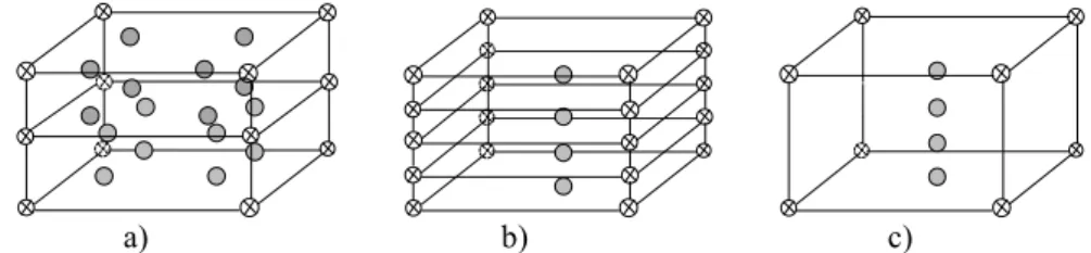
The use of a conventional solid element requires several element layers to correctly capture bending effects, but multiple layers of finite elements along the thickness direction increases the computation time. Figure 6 presents the advantage of RESS finite element structure compared with different finite elements integration scheme. In the Figure 6, all formulations lead to 4 integration points through thickness directions, but the computational effect decrease from a) to b) and from b) to c).

a) b) c)

Figure 6 – Comparison between (a) fully integrated, (b) reduced integrated and (c) RESS formulation, regarding the number of integration points.

In general, the main aspects previously described contribute to the computational advantages of this formulation. The choice of a solid-shell element to simulate sheet metal forming operations is also based on the possibility to use a general constitutive law, while classical shell finite elements are implicitly based on plane stress assumptions. Additionally, thickness variations and double-sided contact conditions are easily and automatically considered with solid-shell finite elements.

5. Line test benchmark

In this section, a simple test is used to assess the effectiveness of adaptive remeshing parameters combined with RESS formulation described in the previous section.

The test description is based on the work of Bouffioux et al. (2008). It consists of a line test using a SPIF machine where a square metallic sheet, with a thickness of 1.2 mm and clamped along its edges, is plastically deformed. The friction coefficient between the tool and the sheet is assumed to be equal to 0.05, and the tool radius is 5 mm. The different stages of the experimental test are schematically illustrated in Figure 7.

Figure 7 – Schematic description of the experimental setup (Bouffioux et al, 2008).

The complete tool path is composed by five steps with an initial tool position tangent to the sheet surface: starting with an indentation of 5 mm (step 1), a linear motion at the same (constant) depth along the X axis occurs (step 2). After that, a second indentation takes place, down to the depth of 10 mm, relatively to the initial position (step 3). Then, a new linear motion (now backwards along the X axis) is imposed, again at a constant depth (step 4), and finally an unloading stage (step 5, not shown in the picture) occurs and brings the tool to its initial position.

The material chosen for the sheet is an aluminium alloy AA3003-O. The material behaviour is elastically described by E = 72600 MPa and ν = 0.36. The hardening parameters for the plastic range are described by a Swift’s law. The material parameters sets used in the current work were the parameters selected from the work of Henrard et al. (2010), for 3D solid finite elements. These material parameters

were achieved using identification methods (Henrard et al., 2010). Among those results available in the literature, one material set was carefully selected to perform the line-test simulations.

Table 1 – Constitutive parameters for an aluminium alloy AA3003-O (Henrard et al., 2010).

Name and hardening type Yield surface coefficients Swift parameters

Hill + Isotropic hardening F=1.224; G=1.193; H=0.8067; N=L=M=4.06 K=183; n=0.229; ε0=0.00057

The relevance of this test is the following: it generates stress and strain values similar as the ones present in incremental forming, even the “extreme” ones as step down of 5mm, which are strongly higher than in classical formed components. The comparison is only related to one constitutive model selected, Table 1, as it was optimum compared to the experimental.

5.1. Numerical Simulations

The main numerical outputs presented in this section are related with the final shape of the sheet, the cross-section along the symmetric axis and the evolution of the tool force achieved. The forming forces (reaction force on the spherical tool) and the deformed shape come from the experimental analysis of Bouffioux et al. (2008). These results will be considered as the reference data in the following sections, to be compared against the numerical simulations.

To assess the influence of the number of integration points along the thickness direction, numerical simulations were carried out with RESS finite element, as presented in the work of Sena et al. (2011). The obtained results showed no variation concerning the different number of integration points adopted (for a range from 3 to 10 points). This is possibly due to the deformation mechanism present, dominated by membrane components even if bending is present. The number of integration points through the thickness chosen for the current work is 5 Gauss points (GP).

Figure 8 illustrates two distinct mesh refinements. The initial refined mesh is composed by 806

elements disposed in one layer in the thickness direction. The coarse mesh used with adaptive remeshing method is composed by 72 elements on the sheet’s plane with one layer of solid-shell elements in the thickness direction. The nodes at the top layer of both meshes define the contact element layer at the surface. The contact modelling is based on a penalty approach at each integration point and on a Coulomb’s law (Habraken and Cescotto, 1998). Finally, the initially refined (reference mesh) and the coarse meshes have two layers of elements (the solid-shell and the contact elements) in the thickness direction, i.e., the total number of elements are 1612 and 144 elements, respectively.

Figure 8 – Reference mesh and coarse mesh used with adaptive remeshing.

The following results are based on the computation of the errors between the experimental measurements and the numerical predictions. The influences of adaptive remeshing parameters are evaluated for the final shape, CPU time and the reaction force of the tool. The force error is determined during the tool loading steps.

The purpose of the next section is to search the optimal adaptive remeshing parameters values in order to use them in future SPIF numerical simulations with the current remeshing technique described in Section 3.

5.1.1. Sensitivity analysis of remeshing parameters

This section provides the analysis of adaptive remeshing parameters which allow the best approximation to the experimental measurements. The simulations were performed to verify the parameters influence in the numerical results. Different values for each parameter were tested for derefinement distance (d) as well the vicinity size (α): d were 0.005mm, 0.05mm, 0.1mm and 0.2mm; α coefficient were 0.1, 0.6, 0.8 1.0 and 1.6. The value of n (number of nodes inserted in one edge) adopted was 3, from preliminary tests using the line-test benchmark.

The final results choices are based in the parameters values which allow less accuracy error for each combination of adaptive remeshing parameters. The relative error average is computed using the following expression: 2 2 i=1 (Num. - Exp.) Error(%) = * 100 Exp. N N _ _{ }  _{  }             

∑

where Num. is the numerical value, Exp. is the experimental value and N is the number of points in X axis (Figure 7). The difference between the numerical value and the experimental is computed for the common abscise values, X axis presented in Figure 7. The numerical values in the X axis were linearly interpolated to match the corresponding X values of experimental measurements.

The following figures exhibit the sensitivity results for different combination values between α coefficient and d parameter using the line test benchmark.

Axial force Shape Total force CPU time 0 2 4 6 8 10 12 14 16 0 0,1 0,2 0,3 0,4 0,5 0,6 0,7 0,8 0,9 1 1,1 1,2 1,3 1,4 1,5 1,6 1,7 α coef. E rr o r (% ) 0 100 200 300 400 500 600 700 800 900 1000 1100 C P U t im e (s )

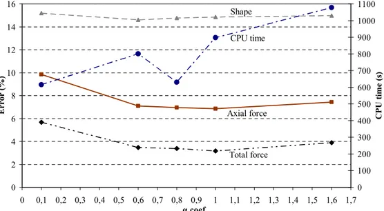
Figure 9 – CPU time and error sensitivity in the prediction of forces and shape for d equal to 0.2 mm. Increasing the value of α coefficient with d equal to 0.2 mm, the error of force prediction tends to decrease with more significance than the shape error. In terms of CPU performance, generally the time increases but there is an exception when the α coefficient is equal to 0.8. Increasing the value of the α parameter, the number of generated new elements increases during the remeshing procedure, and consequently, the CPU time increases. However, the adaptive remeshing parameters affect also the convergence performance during the simulation. This is due to the fact that the number of iterations performed decreases and directly reduces the simulation time. In this case, α is equal to 0.8, which allows better convergence performance, has similar CPU time compared with α equal to 0.1, which allows the generation of less number of elements during the adaptive remeshing method.

Axial force Shape Total force CPU time 0 2 4 6 8 10 12 14 16 0 0,1 0,2 0,3 0,4 0,5 0,6 0,7 0,8 0,9 1 1,1 1,2 1,3 1,4 1,5 1,6 1,7 α coef. E r r o r ( % ) 0 100 200 300 400 500 600 700 800 900 1000 1100 C P U t im e ( s)

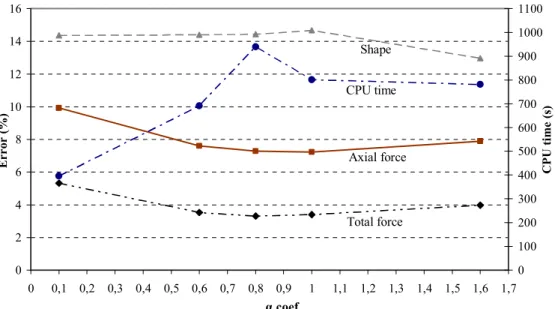
Figure 10 – CPU time and error sensitivity in the prediction of forces and shape for d equal to 0.1 mm. When d parameter is equal to 0.1 mm the force error decreases when the value of α coefficient increases until α value equal to 1 which enables lowest error. The error concerning the shape prediction decreases with α parameter higher than 1.0. In terms of CPU time, generally the time increases for increased α values. In Figure 10, the combination of α value equal to 0.8 and d equal to 0.1mm, the CPU time has an opposite behaviour in comparison with previous results of d equal to 0.2 presented in Figure 9. Axial force Shape Total force CPU time 0 2 4 6 8 10 12 14 16 0 0,1 0,2 0,3 0,4 0,5 0,6 0,7 0,8 0,9 1 1,1 1,2 1,3 1,4 1,5 1,6 1,7 α coef. E r r o r ( % ) 0 100 200 300 400 500 600 700 800 900 1000 1100 C P U t im e ( s)

Figure 11 – CPU time and error sensitivity in the prediction of forces and shape for d equal to 0.05 mm. When d is equal to 0.05 mm, the values of α parameter which allow lowest error are between 0.6 and 1.0. The error determination for the shape prediction decreases for α value higher than 1. The CPU time has the tendency to increase with the α coefficient. However, at the intermediate values of the α parameter (0.8 and 1.0), the CPU time is lower than with α value equal to 0.6, showing again an effect of convergence efficiency related to specific values of remeshing parameters.

Axial force Shape Total force CPU time 0 2 4 6 8 10 12 14 16 0 0,1 0,2 0,3 0,4 0,5 0,6 0,7 0,8 0,9 1 1,1 1,2 1,3 1,4 1,5 1,6 1,7 α coef. E r r o r ( % ) 0 100 200 300 400 500 600 700 800 900 1000 1100 C P U t im e ( s)

Axial Force error(d=0.005mm) Shape error (d=0.005mm)

Figure 12 – CPU time and error sensitivity in the prediction of forces and shape for d equal to 0.005 mm. Figure 12 demonstrates similar results as the previous ones using d equal to 0.005 mm, which nearly prevents any derefinement. These simulations should be the most accurate for shape, however they show that the shape error value stabilizes for all values of d lower than 0.2 mm similar shape errors was reached. The CPU time seems to be quite stable (d = 0.05 mm) or to decrease (d=0.1 mm; 0.005 mm) when α value is higher than 1.0 combined with d values lower than 0.2 mm. The common aspect in all results is that the average error for total force prediction is lower than the average error of axial force. The load in axial force (Z direction) can be influenced by high accuracy of tangential forces, from X and Y directions (Figure 7), and its values remains stabilized for the same values of α parameter.

The following figures exhibit the adaptive remeshing parameters sensitivity error of CPU time time, force and shape predictions in a different perception manner. The error is exhibited in the following figures in function of d values for different α coefficients.

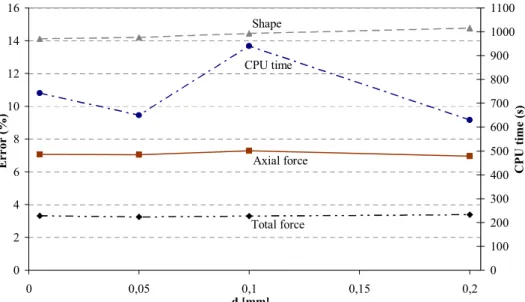
Axial force Shape Total force CPU time 0 2 4 6 8 10 12 14 16 0 0,05 0,1 0,15 0,2 d [mm] E r r o r ( % ) 0 100 200 300 400 500 600 700 800 900 1000 1100 C P U t im e ( s)

Figure 13 – CPU time and error sensitivity in the prediction of forces and shape for α coefficient equal to 0.1. The combination of α coefficient equal to 0.1 with different d values enables higher error than the others values chosen in the prediction of axial force and total force. In contrast, the CPU times to perform the simulations are low. With low value of α coefficient, the mesh area of refinement is small. Consequently, the number of coarse elements included in the refinement is minimal, as the total number of elements.

Analyzing figures 14, 15 and 16 for α values ranging from 0.6 to 1.0, it is verified that the error prediction of shape, axial force and total force are analogous with negligible difference between each parameters set. The only differentiation is the CPU time spent to perform each simulation.

Axial force Chape Total force CPU time 0 2 4 6 8 10 12 14 16 0 0,05 0,1 0,15 0,2 d [mm] E r r o r ( % ) 0 100 200 300 400 500 600 700 800 900 1000 1100 C P U t im e ( s)

Figure 14 – CPU time and error sensitivity in the prediction of forces and shape for α coefficient equal to 0.6.

Axial force Shape Total force CPU time 0 2 4 6 8 10 12 14 16 0 0,05 0,1 0,15 0,2 d [mm] E r r o r ( % ) 0 100 200 300 400 500 600 700 800 900 1000 1100 C P U t im e ( s)

Axial force Shape Total force CPU time 0 2 4 6 8 10 12 14 16 0 0,05 0,1 0,15 0,2 d [mm] E r r o r ( % ) 0 100 200 300 400 500 600 700 800 900 1000 1100 C P U t im e ( s)

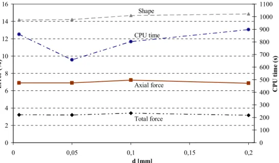
Figure 16 – CPU time and error sensitivity in the prediction of forces and shape for α coefficient equal to 1.0.

Figure 17 presents distinct values of error prediction for shape, axial force and total force in comparison with the combination sets exhibited above, Figure 13 to Figure 16. The error of shape prediction is lower than the previous parameters combination. The adaptive remeshing parameters which presents less shape prediction error is α coefficient equal to 1.6 combined with d value lower or equal to 0.1mm. Using α coefficient equal to 1.6 combined with d value equal to 0.2mm, the shape error is comparable as the previous results. However, the axial force prediction and total force prediction show higher error in relation to numerical results obtained previously.

Axial force Shape Total force CPU time 0 2 4 6 8 10 12 14 16 0 0,05 0,1 0,15 0,2 d [mm] E r r o r ( % ) 0 100 200 300 400 500 600 700 800 900 1000 1100 C P U t im e ( s)

Figure 17 – CPU time and error sensitivity in the prediction of forces and shape for α coefficient equal to 1.6.

In general, the choice of adaptive remeshing parameters values for α coefficient has more effect on the force prediction than the d parameter. Analysing the shape prediction error of all figures in function of d parameter, it is verified that this result is more sensitive to d than to α coefficient. The simulation performance is affected by the adaptive remeshing parameters using different combination values for d and α parameters. A combination of a high α coefficient with small value of d parameter, it allows a huge number of new remeshing elements at the end of the simulation. However, in the particular case of line-test benchmark it does not mean that the simulation is slower due to the better convergence and performs less number of iterations in the FE analysis.

Figure 18 illustrates the number of elements and nodes evolution during the adaptive remeshing procedure. The adaptive remeshing parameters chosen were: α coefficient is equal to 1.6, d parameters equal to 0.2mm and n equal to 3 nodes per edge.

140 240 340 440 540 640 740 0 0,2 0,4 0,6 0,8 1 1,2 1,4 1,6 1,8 Time step U n it [ N u m b e r ]

Number of elements Number of nodes

Figure 18 – Evolution of number of elements and nodes during the adaptive remeshing procedure. The minimum number of elements and nodes are 144 elements and 189 nodes, respectively. The number of elements and nodes varies during the tool motion. When the step 4 (see Figure 7) is executed the number of elements increases due to the higher level of mesh distortion. Figure 19 presents the final number of elements for each combination of α with d parameters for a constant number of nodes divisions per edge (n) equal to 3.

400 720 784 784 848 400 720 752 784 848 400 592 656 656 784 400 496 560 560 624 300 350 400 450 500 550 600 650 700 750 800 850 900 0,1 0,6 0,8 1 1,6 α coef. N º o f e le m e n ts

Nº of elements (d=0.005) Nº of elements (d=0.05) Nº of elements (d=0.1) Nº of elements (d=0.2) Figure 19 – Final number of elements for different pair combination of remeshing parameters.

As mentioned, d equal to 0.05 mm or equal to 0.005 mm presents similar results even for the final number of elements. Exceptionally with α equal to 0.8 the final number of elements is different for both values chosen for d parameter. However, for the different values of d parameter for an equal value of α coefficient, demonstrates that the d parameter has influence in the final number of elements.

Analysing the results sets provided by the sensitivity analysis, the intermediate values were chosen. In terms of force prediction, α parameter exposes better accuracy using the intermediate values [0.6, 0.8 and 1.0] for each combination with d parameter. However, the intermediate values attributed to α parameter shows less accuracy in terms of shape prediction. The shape prediction has better accuracy

when the value of α coefficient is 1.6 and d parameter is smaller than 1.0 mm. Globally, the error of shape prediction presents a smaller difference between each combination of parameters than the error obtained for the force prediction. In this sense, the final choice should be an attribution of an intermediate value for α coefficient. The values of adaptive remeshing parameters selected are: α coefficient equal to 1.0 and for d parameter two different values were selected, which are 0.05 mm and 0.1 mm. These two values will be analysed in the following section in the forming of a conical geometry. The number of nodes division per element’s edges (n) will be also analysed with details in the next section.

Table 2 shows the performance for different adaptive remeshing parameters selected from the previous results and reference mesh (initial mesh refinement).

Table 2 – Average error of shape and force prediction.

Adaptive remeshing Total force error (%)

Axial force error (%) Shape error (%) CPU time (s) α = 1.0 and d=0.05mm 3.192 6.899 14.218 658.176 α = 1.0 and d=0.1mm 3.406 7.232 14.672 801.513 Reference mesh 5,347 3,078 13,557 2300,819

A relative good correlation was obtained between the simulation results and the experimental measurement using both mesh refinement strategies. The comparisons between the numerical results obtained with adaptive remeshing method and with the reference mesh are similar. However, the remeshing procedure presents better accuracy for the total force achieved and final shape prediction. The initial refinement mesh has better accuracy (less error) in the axial force and shape predictions. Even for such small SPIF simulation, the computation time is reasonably large using an initial refined mesh. The number of elements in the reference mesh is clearly large and evidences the advantages of adaptive remeshing technique used, obtaining similar numerical results with less computation time.

6. Simulation of incrementally formed conical shape

This section updates the results of Sena et al. (2013). The numerical simulation of SPIF addressed in the current section consists into a conical aluminium part from the NUMISHEET 2014 benchmark proposal. It is 45º wall-angle with a depth of 45 mm. The sheet material is an AA7075-O with an initial thickness of 1.6 mm. The backing plate maximum and minimum diameters are 148 mm and 140 mm respectively. The tool tip diameter is 12.66 mm and the tool path is based on successive circles with a vertical step size of 0.5 mm per contour, consisting in 90 vertical steps. The initial tool position is located at the sheet centre with an initial gap between the tool and sheet of 0.5 mm. The experimental tool path point was available. The dimensions of ideal design and backing plate geometry are schematically shown

in Figure 20.

Figure 20 – Forming of a conical shape: geometric dimensions.

The elastic material behaviour is described by the Hooke’s law (E = 72000 MPa and ν = 0.33). The adopted hardening type is isotropic and its parameters for the plastic domain are described by Swift and Voce laws.

Figure 21 exhibits the comparison between the experimental measurements of uniaxial tensile test and the theoretical curves described by the equation of Swift and Voce hardening laws. According to the benchmark proposal data an isotropic behaviour and von Mises is assumed.

0 50 100 150 200 250 300 350 400 0,00 0,10 0,20 0,30 0,40 0,50 0,60 0,70 0,80 True Strain S tr e ss [ M P a ]

Experimental 45º Experimental 90º (TD) Experimental 0º (RD) Theoretical Swift 0º Theoretical Swift 45º Theoretical Swift 90º Theoretical Voce 0º Theoretical Voce 45º Theoritical Voce 90º

Figure 21 – Comparison between the experimental uniaxial tensile test measurements and the theoretical curves using Swift and Voce hardening laws.

In general, the material behaviour in different experimental measurement directions has similar values of stress which leads to consider an approximate isotropic material behaviour. In terms of theoretical hardening description, the Swift hardening law has better approximation to the experimental measurements than the Voce hardening law. The chosen material parameters are listed in Table 4, from the benchmark proposal.

Table 3 – Material parameters.

Test type Test direction Hardening type Parameters

Biaxial tension - Swift law K=335.1MPa; n=0.157; ε0=0.004 Uniaxial tension 0º Voce law K=129,17MPa; n=30.55; σ0=97.4MPa Uniaxial tension 0º Swift law K=386.93MPa; n=0.229; ε0=0.004

6.1. Numerical Simulations

The main numerical outputs presented in the following sections are the final shape of the sheet and the evolution of the tool force in the tool axial direction achieved during the simulation. In order to reduce the computation time, a 45º pie of sheet is modelled and rotational boundary conditions are imposed by displacements on the edges (Bouffioux et al., 2010; Henrard et al., 2010). For isotropic material, the pie mesh with 45º can predict as accurately as the full 360º meshes in terms of shape, thickness and force (Henrard, 2008). The numerical shape prediction is extracted from the cross-section along the middle line (figures 22 and 23) of the 45º pie used within the FE model to avoid inaccuracy due to boundary conditions and taking the abscise as the radius. No distinction was made between X and Y, the numerical results are considered equal in all directions. Finally, Coulomb’s friction coefficient between the tool and sheet is set to 0.01, value suggested in the benchmark proposal. Two meshes were tested: an initially refined mesh (reference mesh) with 5828 elements without the remeshing method and a coarse mesh initially with 410, elements combined with the remeshing technique.

Figure 22 – Reference mesh with 5828 finite elements used to perform a 45º wall angle cone simulation. The values used for each remeshing parameter were chosen based on the line-test benchmark from the previous section. The parameter d is tested with two different values (0.05 mm and 0.1 mm). The number of nodes per edge is also tested for different values (from 1 to 4 nodes). Both adaptive remeshing parameters are analysed for different values to verify their influence and compromise between the CPU time and numerical accuracy. The value of the α coefficient is fixed and equal to 1.0.

Figure 23 presents the coarse mesh used with different numbers of nodes per edge (n), from 1 to 4 nodes.

Figure 23 – Coarse mesh of 410 finite elements used with adaptive remeshing to perform a 45º wall angle cone simulation.

The rotational boundary condition was imposed in order to minimize the effect of missing material at the both edges of the pie. This type of boundary condition (BC) is a link between the displacements of both edges. The main purpose to use the rotational BC is due to the tool motion which always moves in the same direction. The material in the tool vicinity is forced to move inducing the twist effect of the shape around its rotational symmetric axis. The tendency to twist can be simulated using the rotational BC applied at the edges of the pie. The twist effect can’t be predicted using symmetric BC.

Table 4 shows the results obtained with RESS finite element, concerning the final number of elements at the end of the numerical simulation for different level of refinement combined with different values of d parameter.

Table 4 – Final number of elements for different level of refinement.

Nº of nodes per edge (n) Initial nº of elements Final nº of elements for d=0.05 mm Final nº of elements for d=0.1 mm 1 410 1330 1010 2 410 2498 1976 3 410 3994 3322 4 410 6010 5510 Reference 5828 5828 5828 Tool direction Tool direction

6.1.1. Shape and thickness prediction

Figure 24 presents all the numerical results obtained using the adaptive remeshing method in comparison with the numerical results using the reference mesh. The numerical results with adaptive remeshing procedure use d parameter equal to 0.05 mm.

-50 -45 -40 -35 -30 -25 -20 -15 -10 -5 0 5 0 5 10 15 20 25 30 35 40 45 50 55 60 65 70 75 80 Radius [mm] D ep th [ m m ] 0 0,2 0,4 0,6 0,8 1 1,2 1,4 1,6 1,8 T h ic k n es s [m m ]

Bottom and Top n=1 Bottom and Top n=2

Bottom and Top n=3 Bottom and Top n=4

Bottom and Top Reference mesh Thickness n=1

Thickness n=2 Thickness n=3

Thickness n=4 Thickness Reference mesh

Figure 24 – Final shape and thickness prediction using adaptive remeshing with α coefficient equal to 1.0 and d equal to 0.05 mm.

Globally, the shape predictions with different refinement levels have similar results when compared with the reference mesh. The thickness prediction has analogous results compared to the reference thickness. However, the thickness prediction using 1 node per edge presents lower value of thickness in some prediction points in the conical shape wall.

Figure 25 presents the absolute error of shape prediction for different levels of refinement (n) and reference mesh. The average shape error is presented as absolute value computed using the following equation:

2 Error

i=1

Shape (mm) = (Num. - Exp.) N N  _{ }  _{ }  _{ }      

∑

where Num. is the numerical value, Exp. is the experimental value and N is the number of points in radius direction. The difference between the numerical value along the cross section and the experimental for different direction is computed for the common values in radius direction. Previously, the numerical values along of middle cross section in the radius axis were linearly interpolated for the corresponding radius values of experimental measurements.

Two different values assigned to d parameter of the adaptive remeshing procedure are compared. The reference mesh is represented in the following figure with the parameter n as equal to zero (n=0).

0 0,1 0,2 0,3 0,4 0,5 0,6 0 1 2 3 4

Nº of nodes per edge (n)

S h a p e e r r o r [ m m ] 0 5000 10000 15000 20000 25000 30000 35000 40000 45000 C P U t im e ( s) d=0.05mm RD d=0.1mm RD d=0.05mm TD

d=0.1mm TD CPU time d=0.05mm CPU time d=0.1

Figure 25 – Shape prediction error and CPU time for different levels of remeshing refinement and reference mesh.

The shape error was computed for different refinement levels combined with two different values of d parameter. In general, the average shape error is less than 1 mm for all numerical results obtained with different refinement levels, as well as with the reference mesh. The CPU time increases from n equal to 1 until n equal to 4, as expected. However, for n equal to 4 the CPU time is higher than the time spent using an initial refined mesh. The reason is the fact that the number of elements in the tool motion direction is more than the double of the number of elements in the same direction using the reference mesh. In this circumstance the use of 4 nodes per edge (n=4) is not interesting to apply specifically in this example. The solution to decrease CPU time using a high number of nodes per edge with adaptive remeshing procedure is the uses of homogeneous coarse mesh. This means that the number of coarse elements on the tool motion direction should be lower, in order to have at least a similar final number of finite elements in tool motion direction using adaptive remeshing method. In this sense it is possible a reasonable comparison between the initial refined mesh and the coarse mesh with the application of adaptive remeshing procedure using n equal to 4 nodes per edge. The CPU time difference between both values of d parameter is negligible for n equal to 1, 2 and 3. However, the CPU time for n equal to 4 for both d values are significant, for d equal to 0.05 mm the CPU time is higher than d equal to 0.1. A small value of d allows the remaining of remeshing elements during its generation in the coarse mesh. The shape prediction with highest level of refinement does not means that it will provide the best shape accuracy. Using the refinement strategy of adaptive remeshing method, the best number of nodes division per edge (n) is 2 nodes combined with d equal to 0.1 mm. However, none of the case of n value equal to 1 and n equal to 3 combined with d equal to 0.1 mm or d equal to 0.05 mm provides a huge difference. The average errors of shape predictions in transverse direction (TD) and in rolling direction (RD) are similar. Concerning to the CPU time is low compared with the CPU time spent with reference mesh.

The following sections present the numerical results of adaptive remeshing with 2 nodes division per edge combined with d equal to 0.1 mm and α coefficient is equal to 1.0. The adaptive remeshing parameters were chosen based in the number of nodes per edge (n) which allows an acceptable average error in both directions with a good agreement with the CPU time. The comparison with experimental measurements and reference mesh is made.

Figure 26 and Figure 27 present shape and thickness predictions using adaptive remeshing technique. The comparison was performed for different experimental measurement directions, rolling direction (RD) and transverse direction (TD).

-50 -45 -40 -35 -30 -25 -20 -15 -10 -5 0 5 0 5 10 15 20 25 30 35 40 45 50 55 60 65 70 75 80 Radius [mm] D e p th [ m m ] 0 0,2 0,4 0,6 0,8 1 1,2 1,4 1,6 1,8 T h ic k n e ss [ m m ]

Shape prediction (n=2) Bottom layer Experimental shape RD

Experimental thickness RD Thickness prediction (n=2)

Figure 26 – Shape and thickness prediction in the rolling direction (RD) with adaptive remeshing refinement (n=2). -50 -45 -40 -35 -30 -25 -20 -15 -10 -5 0 5 0 5 10 15 20 25 30 35 40 45 50 55 60 65 70 75 80 Radius [mm] D ep th [ m m ] 0 0,2 0,4 0,6 0,8 1 1,2 1,4 1,6 1,8 T h ck n e ss [ m m ]

Shape predict (n=2) Bottom surface Experimental shape TD Experimental thickness TD Thickness prediction (n=2)

Figure 27 – Shape and thickness prediction in the transverse direction (TD) with adaptive remeshing refinement (n=2).

Figure 26 and Figure 27 exhibit a suitable accuracy on the numerical shape prediction in comparison with the experimental measurements. The symmetry assumption for the numerical results in both directions is validated. The differences between the measurements in the transverse direction (TD) and rolling direction (RD) are negligible for a symmetric conical shape.

An analogous analysis was performed for the thickness prediction. The numerical thickness prediction has an acceptable accuracy compared with the experimental results in both measured directions. However, the final thickness experimentally measured is higher than the initial thickness in the central area of the sheet and in the area near the clamped zone of the backing plate. This effect is not predicted in the numerical model because the sliding effect is not considered: the clamped boundary

condition is applied in the mesh limits (figures 22 and 23). The main comparison is the final thickness value along the final wall angle shape, where the higher deformations occur and in that sense the numerical results obtained have reasonable accuracy.

6.1.2. Minor and major plastic strain prediction

The current section presents the minor and major plastic strains in rolling and transverse directions. The obtained numerical results are considered equal for both directions. The comparison of numerical results are performed between the reference mesh and adaptive remeshing procedure using 2 nodes per edge (n=2) in relation to the experimental measurement. Figure 28 and Figure 29 exhibit the results comparison in rolling and transverse directions.

-0,08 -0,06 -0,04 -0,02 0,00 0,02 0,04 0,06 0,08 0,10 0,12 0 10 20 30 40 50 60 70 80 Radius[mm] M in o r p la st ic s tr a in

Minor plastic strain (Reference mesh) Experimental Minor plastic strain RD

Minor plastic strain (n=2) Experimental Minor plastic strain TD

Figure 28 – Minor plastic strain prediction.

-0,05 0,00 0,05 0,10 0,15 0,20 0,25 0,30 0,35 0,40 0,45 0 10 20 30 40 50 60 70 80 Radius[mm] M a jo r p la st ic s tr a in

Major plastic strain (Reference mesh) Experimental Major plastic strain RD

Major plastic strain (n=2) Experimnetal Major plastic strain TD