The final publication is available at link.springer.com
DOI: 10.1007/s11119-013-9332-7
Bayesian Methods for Predicting LAI and Soil Water Content
Majdi Mansouri . Benjamin Dumont . Vincent Leemans . Marie-France Destain
Département des Sciences et Technologies de l’Environnement, Université de Liège (GxABT), 2 Passage des Déportés, 5030 Gembloux, Belgium
mfdestain.ulg.ac.be; tel : +32 (0)81622164; fax : +32(0)81622167
Abstract
LAI of winter wheat (Triticum aestivum L.) and soil water content of the topsoil (200 mm) and of the subsoil (500 mm) were considered as state variables of a dynamic soil-crop system. This system was assumed to progress according to a Bayesian probabilistic state space model, in which real values of LAI and soil water content were daily introduced in order to correct the model trajectory and reach better future evolution. The chosen crop model was mini STICS which can reduce the computing and execution times while ensuring the robustness of data processing and estimation. To predict simultaneously state variables and model parameters in this non-linear environment, three techniques were used: Extended Kalman Filtering (EKF), Particle Filtering (PF), and Variational Filtering (VF). The significantly improved performance of the VF method when compared to EKF and PF is demonstrated. The variational filter has a low computational complexity and the convergence speed of states and parameters estimation can be adjusted independently. Detailed case studies demonstrated that the root mean square error (RMSE) of the three estimated states (LAI and soil water content of two soil layers) was smaller and that the convergence of all considered parameters was ensured when using VF. The interest of assimilating measurements in a crop model allows accurate prediction of LAI and soil water content at a local scale. As these biophysical properties are key parameters in the crop-plant system characterization, the system has the potential to be used in precision farming to aid farmers and decision makers in developing strategies for site-specific management of inputs, such as fertilizers and water irrigation.
Keywords Crop model . Bayes . Soil water content . LAI . Data assimilation . Extended Kalman
Introduction
Up to now, despite the wide development of agricultural technology, decisions regarding field management are still made by the farmer (Hautala and Hakojarvi, 2011). There is thus a need for decision making systems furnishing strategies for effective management of inputs, such as fertilizers and irrigation water. Leaf area index (LAI) and soil water content are key parameters within this scope (Behera and Panda, 2009). LAI is the total one-sided area of leaf tissue per unit ground surface area (square meters per square meter). It determines the water and gas exchanges, and consequently influences the photosynthetic primary production and plant growth. Soil water content is the content of water in the soil, held in the spaces between soil particles. It greatly influences the processes related to plant growth and agricultural production since it affects the capacity of plants to extract water and soil nutrients. The prediction of soil water content is important for management practices, such as nitrogen redistribution or irrigation. In this paper, the prediction of LAI and soil water content relies on the fact that they are considered as state variables of a crop model. Indeed, a dynamic crop model analyses the temporal evolution of state variables as a function of input variables including soil and crop characteristics, management practices (namely, nitrogen supply), and climate variables. Nevertheless, accurate prediction of state variables is not straightforward in these models. Most of the equations describing the evolution of state variables are non-linear approximations of biophysical processes. For example, the evolution of LAI comprises three phases, growth, stability, and senescence described by different formalisms according to the models (Palosuoa et al., 2011). In STICS for example, these three phases are respectively described by logistic, constant and linear equations (Brisson et al., 2003). Uncertainties affect the input variables. Common problems encountered include mis-calibration or poor maintenance of instruments, weather inputs taken too far from the experimental site and soil properties defined from published data soil series rather than field measurement (Bellochi et al., 2009). The importance of accurate soil and weather input data increases as the environment becomes more limiting for plant growth and development (Weiss and Wilhem, 2006). Measurement uncertainties on the outputs have also important implications for model calibration and validation. As a consequence of the non-linearity, the state variables do not have a Gaussian distribution, even if all the errors are normally distributed.
For these reasons, it is interesting to modify the model during the crop lifecycle to make it a better predictor for a specific situation, such as a given agricultural field (Makowski et al., 2004). Clearly, this implies introducing measurements of state variables such as the LAI and the soil water content in the model in order to estimate its accuracy and achieve better prediction.
Regarding measurements, several methods have been developed to quantify LAI at the field scale (Jonckheere et al., 2004). The reference method, which involves harvesting the vegetation and measuring the area of all leaves within a delimitated area, is destructive. Other methods that infer LAI from measurements of the transmission of radiation through the canopy (Breda, 2003) are non-destructive. For example, the Plant Canopy Analyser LAI 2000 (Li-COR, Lincoln, USA) is easy-to-apply and is often used to estimate the LAI indirectly. Its main drawback is due to the fact that the sensor cannot get totally underneath low-level canopies. To solve that problem, Van Wijk and Williams (2005) combined field measurements of canopy reflectance (NDVI) and light penetration through the canopy (gap-fraction) and obtained accurate non-destructive assessment of the variability of LAI in low level vegetation. More recently, methods have been proposed to obtain real-time data processing of LAI. Gebbers et al (2011) developed a rapid mapping of the LAI on the basis of ground-based laser rangefinders mounted on a vehicle. Sakamoto et al. (2012) applied a camera-based observation system using vegetation indices for monitoring of seasonal changes in several biophysical parameters of maize such as
LAI. Leemans et al. (2012) explored the potential of a stereo vision device to measure the LAI at different growth stages of wheat. In these three cases, the accuracy of the estimation was comparable to that obtained by commercial sensors. From these research studies, it appears that ground-based non-invasive sensors will become affordable in the near future to evaluate the spatial and temporal variability of LAI with an acceptable accuracy and a reduced work load.
A review of the available methods available for estimating soil water content is given by Dobriyal et al. (2012). The reference method is destructive and involves oven drying a soil sample of known volume at 105 °C for 24 h. The water content is calculated by subtracting the oven dry weight from the initial field soil weight (Lunt et al., 2005). Besides methods based on radioactivity, measurement of the capacitance between soil-implanted electrodes, time domain reflectometry (TDR) and ground penetrating radar (GPR) methods are widely used. More recently, large arrays of sensors (using wireless sensors networks to transmit the data) developed for the field measurement of soil water content have been shown to be able to characterize
automatically the spatio-temporal variability of soil water content (Stacheder et al., 2009; Zhang et al., 2011; Sudha et al., 2011). Low-cost and low-power sensors are distributed in the field and are included in platforms that efficiently integrate the measurement of soil water content (measurement of the capacitance between soil-implanted electrodes) and the data transmission to the end-user (even over long distances, typically several kilometers).
With regard to the algorithms, the introduction of measurements of state variables such as the LAI and the soil water content in to the model in order to correct ‘its trajectory’ and achieve better prediction may be considered as an optimal filtering problem. This consists of recursively updating the posterior distribution of the unobserved state given the sequence of observed data and the state evolution model. The filtering problem has been addressed with several methods, such as the Kalman Filter (KF) which provides an optimal Bayesian solution but is limited by the non-universal Gaussian modeling assumptions. An application of this technique to a linear dynamic crop model predicting a single state variable, the winter wheat biomass, was presented by Makowski et al. (2004). The authors showed how the model predictions can be sequentially updated by using several measurements, and studied the sensitivity of the results to the variance of the model errors. The Ensemble Kalman Filtering (EnKF) (Xiao et al., 2009), Extended Kalman Filtering (EKF) (Calvet, 2000), and the Unscented Kalman Filtering (UKF) (Van Der Merwe & Wan, 2001) have been proposed to improve the KF flexibility. Xiao et al. (2009) developed a real-time inversion technique to estimate LAI from time series reflectance data using a coupled dynamic and radiative transfer model.
Other state estimation techniques use a Bayesian framework to estimate the state and/or parameter vector. This approach relies on computing the probability distribution of the unobserved state given a sequence of the observed data in addition to a state evolution model. Consider an observed data set y which is generated from a model defined by a set of unknown state variables and/or parameters z. The information about the data are completely expressed via the parametric probabilistic observation model P
( )
yz . The randomness of a process can be solved by constructing a distributionP( )
zy , called the posterior distribution, which quantifies the information about the system after obtaining the measurements. According to Bayes theorem, the posterior can be expressed as( )
( )
( )
( )
y P z P z y P y z P = (1)whereP
( )
yz is the conditional distribution of the data given the vector z, which is called the likelihood function, P( )
z is the prior distribution which quantifies the information about z before obtaining the measurements, and P( )
y is the distribution of the data. Unfortunately, for most non-linear systems and non-Gaussian noise observations, closed-form analytic expressions of the posterior distribution of the state vector are intractable (Kotecha and Djuric, 2003). To overcome this drawback, a non-parametric Monte Carlo sampling-based method called Particle Filtering (PF) was proposed by Doucet and Tadic (2003). The latter method presents several advantages since: (i) it can account for the constraint of a small number of data samples, (ii) the online update of the filtering distribution and its compression are simultaneously performed, and (iii) it yields an optimal choice of the sampling distribution over the state variable by minimizing the Kullback-Leibler (KL) divergence (MacKay, 2003).Recently, a variational filtering (VF) has been proposed for solving the non-linear parameter estimation problem (Mansouri et al., 2009) but, until now, the method has been applied only for tracking/localization in wireless sensor network problems. The variational filter can be applied to large parameter spaces, has better convergence properties and is easier to implement than the particle filter. Both of them can provide improved accuracy over the extended Kalman filter. Nevertheless, some practical challenges can affect the accuracy of estimated states and/or parameters, namely the presence of measurement noise in the data, the restricted availability of the measured data samples and the larger number of model parameters.
The objectives of the paper are to compare three filtering methods to estimate the temporal evolution of LAI and soil water content of two soil layers (topsoil, 200 mm and subsoil, 500 mm) during the whole plant lifecycle: the Extended Kalman Filtering, the Particle Filtering and the Variational Filtering. In this investigation, the state vector to be estimated at any time instant is assumed to follow a Gaussian model, where the expectation and the covariance matrix are constants. The comparison relies on the computation of the RMSE and the number of parameters that can be accurately predicted. The basic crop model used in this study is mini STICS (Tremblay and Wallach, 2004; Makowski et al., 2004) which has several advantages since it can reduce the computing and execution times and has the nice property of being a good dynamic model, ensuring the robustness of data processing and estimation.
Materials and methods
Problem Statement
A crop model can be described by a discrete set of equations:
(
)
(
k k k k)
k k k k k k v , , u , x h y w , , u , x f x θ θ = = −1 −1 −1 −1 (2)where k is an index corresponding to the time, xk is the vector of state variables, utis the vector
of input variables, θtis a parameter vector, yk is the vector of the measured variables, wtand vt
are respectively model and measurement noise vectors, g and l are non-linear differentiable functions, the first one determines the new state variables as a function of the preceding situation, while the second expresses the dependence of the measurements. It is assumed that the error terms wtand vt have normal distributions with zero expectation, and that they are mutually
independent.
Estimating the state vectorxk, as well as the parameter vector θk, it is assumed that the parameter vector is described by the following model:
1 1 − − + = k k k θ γ θ (3)
where
γ
k−1 is white noise. In other words, the parameter vector model (3) corresponds to a stationary process, with an identity transition matrix, driven by white noise. A new state vector is defined that augments the two vectors together as follows:(
)
+ = = − − − − − 1 1 1 1 1 k k k k k k k k w , u , x f x z γ θ θ (4)where zk is assumed to follow a Gaussian model where at any time k the expectation µk and the
covariance matrix λk are both constants. Also, defining the augmented vector,
= − − − 1 1 1 k k k w γ ε (5)
(
−1 −1 −1)
ℑ = k k k k z ,u , z ε(
k k k)
k z ,u , y =ℜ ν (6)where ℑ and ℜare differentiable non-linear functions.
General State Evolution Model (GSEM)
In this paper, a general state evolution model GSEM (Mansouri et al., 2009) is employed instead of the kinematic parameter model (Kotecha and Djuric, 2003) usually used in tracking problems. In fact, the GSEM model is more practical for non-linear and non-gaussian situations where no a priori information on the state value is available. The state variable zk at instant k is assumed to follow a Gaussian model, where the expectation µk and the precision matrix λk are both random. Gaussian distribution for the expectation and Whishart distribution for the precision matrix form a practical choice for the filtering implementation. The hidden state zk is extended to an augmented state α =k
(
zk,µk,λk)
, yielding a hierarchical model as follows,k µ ∼N
(
µk µk−1,λ)
k λ ∼W(
λkS)
k z ∼N(
µkλk)
(7)where the fixed hyper-parameters λ,S and nare respectively the random walk precision matrix, the degrees of freedom and the precision of the Wishart distribution. Note that assuming random mean and covariance for the state zk leads to a prior probability distribution covering a wide range of tail behaviors allowing discrete jumps in the state variable.
In fact, the marginal state distribution is obtained by integrating over the mean and precision matrix: k k k k k k k k k k|z ) p(z | , )p( , |x )d z ( p −1 =
∫
µ λ µ λ −1 µ λ (8)where the integration with respect to the precision matrix leads to the known class of scale mixture distributions introduced by Barndorff-Nielsen (Kotecha and Djuric, 2003). Low values of the degrees of freedom n reflect the heavy tails of the marginal distributionp(zk|zk−1).
Variational Bayesian Filter
The variational approach consists in approximating p(αk|z1:k) by a separable distribution
) ( q ) ( q ) x ( q ) (
q αk = k µk λk that minimizes the Kullback-Leibler divergence (DKL) between the
true filtering distribution and the approximate distribution,
( )
( )
( )
(
)
∫
= k k : k k k KL d p q log q p q D α α α α α 1 (9)The minimization is subject to constraint
∫
q( )
αk dαk = 1. The Lagrange multiplier method usedin Vermaak et al. (2003) shows that the updated separable approximating distribution q(αk)
has the following form:
) , ( N ) | ( q ) S | ( W ) ( q ) , | ( N ) ( q ) , | z ( N ) z | y ( p ) z ( q p k p k k k * k k n k * k * k k k k k k k k k λ µ µ µ λ λ λ µ µ µ λ µ ∝ ∝ ∝ ∝ −1 (10)
where .q denotes the expectation operator relative to the distribution q. The parameters are
iteratively updated according to the following scheme:
(11)
In fact, taking into account the separable approximate distribution at time k−1, the predictive distribution is written, ) ( ) S z z z z ( S n n ) z ( * k p k * k p k T k k T k k T k k T k k * k * p k k * k p k p k k k * k * k 1 1 1 1 1 1 1 1 − − − − − − − + = = + + + − = + = + = + = λ λ λ µ µ µ µ µ µ λ λ λ λ µ λ λ µ
) ( q ) | , z ( p d ) ( q ) | ( p ) z | ( p k p k k k k k k k k : k µ µ λ α α α α α ∝ ∝ − − − − −1 1 1
∫
1 1 1 (12)The exponential form solution, which minimizes the Kullback-Leibler divergence between the predictive distribution p(αk|z1:k−1) and the separable approximate distribution qk|k−1(α), yields Gaussian distributions for the state and its mean and Wishart distribution for the precision matrix: ) n , V ( N ) ( q ) , ( N ) ( q ) , ( N ) z ( q * * n k k | k * * k k | k q k q k k k | k k | k k | k k | k k | k k | k k | k 1 1 1 1 1 1 1 1 1 − − − − − − ∝ ∝ ∝ − − − λ λ µ µ λ µ (13)
where the parameters are updated according to the same iterative scheme as and the expectations are exactly computed as follows:
1 1 1 1 1 1 1 1 1 1 1 1 1 1 1 1 1 1 1 1 1 − − − − − − − − − − − + + + − = + = − + − = − + = + = = − − − − − − ) S z z z z ( S n * k | k n p k k | k k * k k ) z ( ) ( k | k k | k k | k k | k k | k k | k q T k k T q k q k T q k q k q T k k * k p k p k k | k k k | k k * k k * k k * k p k * k p k µ µ µ µ λ λ λ λ µ λ λ µ λ λ λ µ µ (14)
Compared to the particle filtering method, the computational cost and the memory requirements are dramatically reduced by the variational approximation in the prediction phase. In fact, the expectations involved in the computation of the predictive distribution have closed forms, avoiding the use of Monte Carlo integration.
Case study and crop model presentation
The data used in this paper derive from an experiment designed to study wheat growth response (Triticum aestivum L., cultivar Julius) under different nitrogen fertilization levels during the crop season 2008-09. The experimental blocks were prepared on two soil types (loamy and sandy loam), corresponding to the agro-environmental conditions of the Hesbaye region in Belgium. The measurements were the results of four replications by date, nitrogen level and soil type. Each replication was performed on a small block (2 m × 6 m) within the original experiment as a complete randomised block distribution, spread over the field within each soil type, to ensure measurement independence. A wireless micro-sensor network (eKo pro series system, Crossbow Technology, USA) was used to continuously characterize the soil at two depths (200 and 500 mm) and the atmosphere within the vegetation. Six eKo nodes supporting sensors were implemented throughout the experimental blocks, on the two soil types. The following biophysical variables were measured: water content (EC-5, Decagon, USA), soil moisture potential and soil temperature (eS1101, Watermark, USA), ambient relative humidity and air temperature (SHT7x, Sensirion, Switzerland), global radiation (6450, Davis, USA). A weather station (ES2000, MEMSIC, USA) was also implemented in the experimental field in order to measure wind speed, wind direction and pluviometry. LAI, biomass, and soil nitrogen content were regularly measured manually.
The model for which the methods were tested is Mini STICS model (Makowski et al., 2004). Its structure can be derived from the basic conservation laws, namely material and energy balances. It contains dynamic equations that indicate how each state variable evolves from one day to the next as a function of the current values of the state variables, of the input variables and of the parameter values. Encoding these equations over time allows one to eliminate the intermediate values of the state variables and relate the state variables at any time to the explanatory variables on each day up to that time. However, the model involves several parameters that are usually not known, which include the radiation use efficiency expressing the biomass produced per unit of intercepted radiation, the maximal value of the ratio of intercepted to incident radiation and the coefficient of extinction of radiation. The model parameters determined by Makowski et al. (2004) are shown in Table 1.
Problem Formulation
Based on the equations described in Makowski et al. (2004), the mathematical model LSM of the LAI and soil water content is given by:
( )
(
(
)
)
( )
(
(
)
)
( )
(
(
)
θ)
θ θ + − = + − = + − = 1 2 2 1 1 1 1 3 2 1 t HUR f t HUR t HUR f t HUR t LAI f t LAI (15)where t is the time, f1−3 are the corresponding model functions, and θ is the vector of parameters driving the simulations (Table 1). LAI is the leaf area index and HUR1 (resp. HUR2) is the volumetric water content of layer 1 (resp. layer 2). Discretizing the model (15) using a sampling interval of ∆t (one day), one obtains:
( )
[
]
( )
[
]
( )
[
]
3 1 1 3 2 1 1 2 1 1 1 1 2 2 1 1 − − − − − − + + ∆ = + + ∆ = + + ∆ = k k k k k k k k k w HUR t g HUR w HUR t g HUR w LAI t g LAI θ θ θ (16) where j ( ) ,..., jw∈1 3 is a process Gaussian noise with zero mean and known variance 2
j
γ
σ . Up to now,
model (16) assumes that the parameter θ is constant. These parameters are ADENS, DLAIMAX, and PSISTURG. ADENS is a parameter of compensation between stem number and plant density. In the case of wheat, it is the tillering ability. DLAIMAX is the maximum rate of the setting up of
LAI and PSISTURG is the absolute value of the potential of the beginning of decrease in the cellular extension. For estimating some (or all) of these parameters, the equations describing their evolution are also needed:
1 1 1 − − + = k k k ADENS ADENS γ 2 1 1 − − + = k k k DLAIMAX DLAIMAX γ 3 1 1 − − + = k k k PSISTURG PSISTURG γ (17)
where j( ) ,..., j∈1 3
γ is a process Gaussian noise with zero mean and known variance 2
j
γ
σ . Combining
(16) and (17), one obtains:
(
)
[
]
1 1 1 1 1 1:LAIk= g k− ∆t+LAIk− +wk− f θ(
)
[
]
2 1 1 1 2 2:HUR1k = g k− ∆t+HUR1k− +wk− f θ(
)
[
]
3 1 1 1 3 3:HUR2k= g k− ∆t+HUR2k− +wk− f θ (18) 1 1 1 4:ADENSk =ADENSk− + k− f γ 2 1 1 5:DLAIMAXk =DLAIMAXk− + k− f γ 3 1 1 6:PSISTURGk =PSISTURGk− + k− f γwhere fk∈(1,...,6) are some non-linear functions and where
(
)
T w , w , w w= 1 2 3 and γ =(
γ1,γ2,γ3)
T are respectively the measurement and process noise vector, which quantify randomness at both levels. In other words, the augmented state: zk =(
xk,θk)
T is formed which is the vector to be estimated. It can be given by a 6 by 1 matrix:( )
( )
( )
k k k k k k HUR ,: x HUR ,: x LAI ,: x 2 3 1 2 1 → → →( )
k k ,: ADENS x 4 → (19)( )
( )
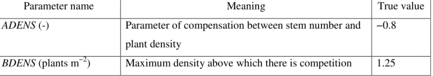
k k k k PSISTURG ,: x DLAIMAX ,: x → → 6 5Table 1. Model parameters (Makowski et al., 2004)
Parameter name Meaning True value
ADENS (-) Parameter of compensation between stem number and
plant density
−0.8
between plants
CROIRAC (mm degree −
day−1)
Growth rate of the root front 2.5
DLAIMAX (m2 leaves m−2 soil degreedays−1)
Maximum rate of the setting up of LAI 0.0078
EXTIN (-) Extinction coefficient of photosynthetically active
radiation in the canopy
0.9
KMAX (-) Maximum crop coefficient for water requirements 1.2
LVOPT (mm root cm−3 s) Optimum root density 5.0
PSISTO (kPa) Absolute value of the potential of stomatal closing 1000
PSISTURG (kPa) Absolute value of the potential of the beginning of
decrease in the cellular extension
400
RAY ON (mm) Average radius of roots 0.2
TCMIN (°C) Minimum temperature of growth 6
TCOPT (°C) Optimum temperature of growth 32
ZPENTE (m) Depth where the root density is 1/2 of the surface root
density for the reference profile
1.20
ZPRLIM (m) Maximum depth of the root profile for the reference
profile
1.50
The abilities of EKF, PF and VF to solve this non-linear state estimation problem are tested through different cases summarized below. In all cases, it is assumed that three states (LAI,
HUR1 and HUR2) are measured. This assumption is realistic since HUR1 and HUR2 are continuously measured by soil water content micro-sensors. Up to now, LAI is obtained by reference measurements but automatic methods are in progress (Gebbers et al., 2011; Leemans et al., 2012; Sakamoto et al., 2012).
i) Case 1: the three states (LAI, HUR1 and HUR2) along with the parameter ADENS are estimated.
ii) Case 2: the three states (LAI, HUR1 and HUR2) along with the parameter ADENS and
iii) Case 3: the three states (LAI, HUR1 and HUR2) along with the parameter ADENS,
DLAIMAX and PSISTURG are estimated.
Sampling data generation
To obtain original dynamic data, the model was first used to simulate the temporal responses LAIk, HUR1k, HUR2k on the basis of the recorded climatic variables. The sampling time used for discretization was 1 day.
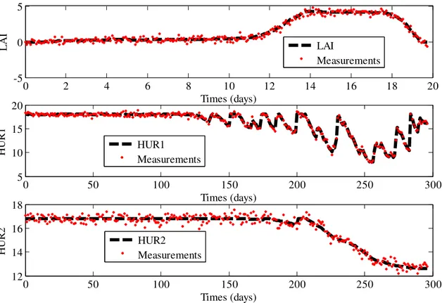
Moreover, to characterize the ability of the different approaches to estimate both the states and the parameters at same time, “true” parameter values were chosen (Table 1). The advantage of working by simulation rather than on real data is that the true parameter values are known. It is thus possible to calculate the quality of the estimated parameters and the predictive quality of the adjusted model for each method. The drawback is that the generality of the results is hard to know. The results may depend on the details of the model, on the way the data are generated and on the specific data that are used. The simulated values, assumed to be noise free, are shown in Figure 1. The evolution of LAI during the wheat’s lifecycle presents the three expected phases, growth, stability and senescence. Daily variations of shallow ground water show fluctuations that were damped in the subsoil layer.
These simulated states were then contaminated with zero mean Gaussian errors, i.e., the measurement noise vk−1~
(
)
2
0, v
Figure 1. Simulated LSM data used in estimation: state variables (LAI leaf area index,
HUR1volumetric water content of the layer 1; HUR2 volumetric water content of the layer
2).
Simulations results analysis
In this section, in the first study, the performance of EKF, PF and VF in estimating the three states, the leaf-area index LAI, the volumetric water content of the layer 1 HUR1 and the volumetric water content of the layer 2 HUR2 are compared.
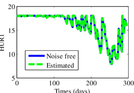
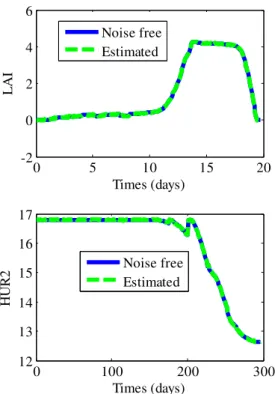
It can be observed from Figures 2, 3 and 4, as well as Table 2, that the VF shows improved estimation performance over EKF and PF. The EKF estimation was not as accurate as the ones corresponding to PF and VF due to the essential limitation of the EKF in non-linear environments. Also, the estimation improvement of VF over PF is due to the fact that the VF
0 2 4 6 8 10 12 14 16 18 20 -5 0 5 Times (days) L A I LAI Measurements 0 50 100 150 200 250 300 5 10 15 20 Times (days) H U R 1 HUR1 Measurements 0 50 100 150 200 250 300 12 14 16 18 Times (days) H U R 2 HUR2 Measurements
yields an optimal choice of the sampling distribution over the estimated state by minimizing the KL divergence.
Figure 2. Estimation of LAI, HUR1, HUR2 using EKF.
0 5 10 15 20 -2 0 2 4 6 Times (days) L A I 0 100 200 300 5 10 15 20 Times (days) H U R 1 Noise free 0 100 200 300 12 13 14 15 16 17 Times (days) H U R 2 Noise free Estimated Noise free Estimated
Figure 3. Estimation of LAI, HUR1, HUR2 using PF. 0 5 10 15 20 -2 0 2 4 6 Times (days) L A I 0 100 200 300 5 10 15 20 Times (days) H U R 1 0 100 200 300 12 13 14 15 16 17 Times (days) H U R 2 Noise free Estimated Noise free Estimated Noise free Estimated
Figure 4. Estimation of LAI, HUR1, HUR2 using VF.
Table 2. Root mean square errors (RMSE) of estimated states
Technique RMSE
LAI HUR1 HUR2
EKF 0.0612 0. 0548 0. 0283 PF 0. 0338 0. 0304 0. 0242 VF 0. 0179 0. 0154 0. 0111 0 5 10 15 20 -2 0 2 4 6 Times (days) L A I 0 100 200 300 5 10 15 20 Times (days) H U R 1 0 100 200 300 12 13 14 15 16 17 Times (days) H U R 2 Noise free Estimated Noise free Estimated Noise free Estimated
In the second study, the effect of the number of estimated parameters on the estimation performances of EKF, PF and VF and in estimating the states and parameters of the LSM process model was examined.
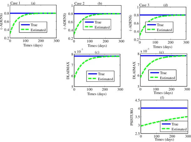
The estimation of the state variables and parameter(s) for these three cases were performed using the three state estimation techniques, EKF, PF and VF. The estimation results for the model parameters using these techniques are shown in Figures 5, 6 and 7, respectively. For example, Figure 5 shows the estimation of the parameters using EKF: Figure 5(a) show the estimates of ADENS, Figure 5(b,c) estimates ADENS and DLAIMAX, and Figures 5(d,e,f) present the estimation of all three parameters ADENS, DLAIMAX, and PSISTURG. Also, Tables 3, 4 and 5 compare the performance of the three estimation techniques for the three cases. For example, for case 1, Table 3 compares the estimation root mean square errors for the three state variables LAI, HUR1 and HUR2 (with respect to the noise-free data) and the mean of the estimated parameter DLAIMAX at steady state (i.e., after convergence of parameter(s)) for different cases using the three estimation techniques.
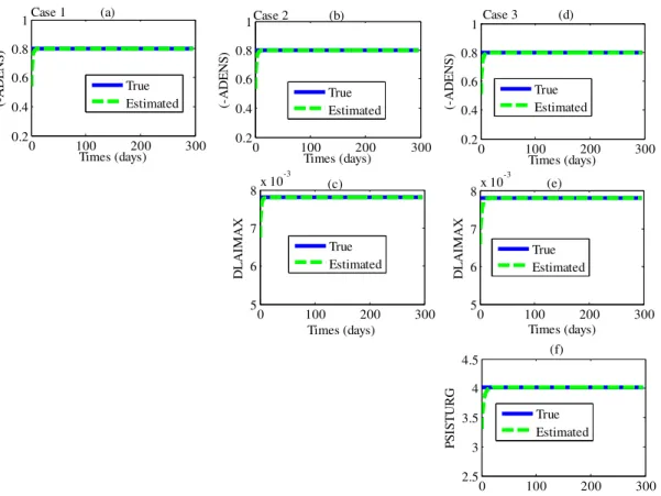
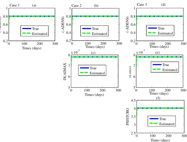
It can be seen from the results presented in Tables 3, 4 and 5 that in all cases, the PF outperformed the EKF (i.e., provides smaller RMSE for the state variables), and that the VF showed a significant improvement over all other techniques. These results confirm the results obtained in the first comparative study, where only the state variables were estimated. The advantages of the VF over the PF (and the PF over the EKF) can also be seen through their abilities to estimate the model parameters. For example, EKF could perfectly estimate one parameter in case 1 (see Fig. 5 (a)), but it took longer to estimate a second parameter in case 2 (see Figures 5(b, c)), and it could not converge for the third parameter in case 3 (see Figure 5(d, e, f)), where it is used to estimate all three parameters. The PF, on the other hand, could estimate all parameters in all cases 1-3, even though it took longer to converge in case 3, where all three parameters were estimated (see Fig. 6). The VF, however, could estimate all parameters in all three cases, and converged faster than all other techniques (see Fig. 7). These advantages of the VF are due to the fact that it provides an optimum choice of the sampling distribution used to approximate the posterior density function, which also accounts for the observed data and the effectiveness of using a general state evolution model.
The results also show that the number of estimated parameters affect the estimation accuracy of the estimated state variables. In other words, for all estimation techniques, the estimation RMSE of LAI, HUR1 and HUR2 increases from the first comparative study (where only the state variables are estimated) to case 1 (where only one parameter, DLAIMAX, is estimated) to case 3 (where all three parameters, ADENS, DLAIMAX, and PSISTURG , are estimated). For example, the RMSEs obtained using EKF for LAI in the first comparative study and cases 1-3 of the second comparative study were 0.0612, 0.0614, 0.0617, and 0.0659 respectively, which increased as the number of estimated parameters increased (refer to Tables 3, 4 and 5). This observation is valid for the other state variables HUR1 and HUR2 and for all other estimation techniques, PF and VF.
Figure 5. Estimation of the LSM model parameters using EKF for all cases - case 1 (ADENS, a), case 2: (ADENS, b and DLAIMAX, c), case 3: (ADENS, d; DLAIMAX, e; PSISTURG, e).
0 100 200 300 0.2 0.4 0.6 0.8 1 Times (days) (-A D E N S ) Case 1 (a) True Estimated 0 100 200 300 0.2 0.4 0.6 0.8 1 Times (days) (-A D E N S ) Case 2 (b) True Estimated 0 100 200 300 5 6 7 8x 10 -3 Times (days) D L A IM A X (c) True Estimated 0 100 200 300 0.2 0.4 0.6 0.8 1 Times (days) (-A D E N S ) Case 3 (d) True Estimated 0 100 200 300 5 6 7 8x 10 -3 Times (days) D L A IM A X (e) True Estimated 0 100 200 300 2.5 3 3.5 4 4.5 Times (days) P S IS T U R G (f) True Estimated
Figure 6. Estimation of the LSM model parameters using PF for all cases - case 1 (ADENS, a), case 2: (ADENS, b and DLAIMAX, c), case 3: (ADENS, d; DLAIMAX, e; PSISTURG, e).
0 100 200 300 0.2 0.4 0.6 0.8 1 Times (days) (-A D E N S ) Case 1 (a) 0 100 200 300 5 6 7 8x 10 -3 Times (days) D L A IM A X (c) 0 100 200 300 0.2 0.4 0.6 0.8 1 Times (days) (-A D E N S ) Case 2 (b) 0 100 200 300 0.2 0.4 0.6 0.8 1 Times (days) (-A D E N S ) Case 3 (d) 0 100 200 300 5 6 7 8x 10 -3 Times (days) D L A IM A X (e) 0 100 200 300 2.5 3 3.5 4 4.5 Times (days) P S IS T U R G (f) True Estimated True Estimated True Estimated True Estimated True Estimated True Estimated
Figure 7. Estimation of the LSM model parameters using VF for all cases - case 1 (ADENS, a), case 2: (ADENS, b and DLAIMAX, c), case 3: (ADENS, d; DLAIMAX, e; PSISTURG, e).
Table 3. Root mean square errors (RMSE) of estimated states and mean of estimated parameters - case 1
Technique RMSE
Mean at steady state
LAI HUR1 HUR2 ADENS
EKF 0.0614 0. 0551 0. 0286 −0.8 PF 0. 0341 0. 0311 0. 0245 −0.8 VF 0. 0182 0. 0157 0. 0115 −0.8 0 100 200 300 0.2 0.4 0.6 0.8 1 Times (days) (-A D E N S ) Case 1 (a) True Estimated 0 100 200 300 0.2 0.4 0.6 0.8 1 Times (days) (-A D E N S ) Case 2 (b) True Estimated 0 100 200 300 5 6 7 8x 10 -3 Times (days) D L A IM A X (c) 0 100 200 300 0.2 0.4 0.6 0.8 1 Times (days) (-A D E N S ) Case 3 (d) True Estimated 0 100 200 300 5 6 7 8x 10 -3 Times (days) D L A IM A X (e) 0 100 200 300 2.5 3 3.5 4 4.5 Times (days) P S IS T U R G (f) True Estimated True Estimated True Estimated
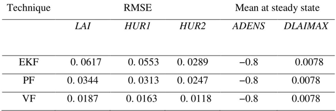
Table 4. Root mean square errors (RMSE) of estimated states and mean of estimated parameters – case 2
Technique RMSE Mean at steady state
LAI HUR1 HUR2 ADENS DLAIMAX
EKF 0. 0617 0. 0553 0. 0289 −0.8 0.0078 PF 0. 0344 0. 0313 0. 0247 −0.8 0.0078 VF 0. 0187 0. 0163 0. 0118 −0.8 0.0078
Table 5. Root mean square errors (RMSE) of estimated states and mean of estimated parameters - case 3
Technique RMSE Mean at steady state
LAI HUR1 HUR2 ADEN
S
DLAIMA X
PSITURG
EKF 0.0659 0. 0585 0. 0291 −0.8 0.0078 did not converge
PF 0.0368 0.0347 0.0276 −0.8 0.0078 4
VF 0.0211 0.0218 0.0172 −0.8 0.0078 4
The effectiveness of daily introduction of measurements of LAI and soil water content into a crop model has thus been demonstrated. Amongst the chosen filtering techniques, the VF method appeared to be the more efficient. For example, in the estimation of soil water content, the maximum value of the RMSE was 2.1 % at 200 mm depth (where the daily fluctuations may be high) while it was 1.7 % at 500 mm depth (where the daily fluctuations are damped).
Besides the accurate prediction of the three state variables LAI, HUR1 and HUR2, the VF method allows estimation of the model’s parameters. Hence, the method has the potential to determine model outputs such as yield, protein content, soil nitrogen content, ...
From a practical point of view, the set up of the method implies the need to distribute sensors able to measure spatial and temporal changes of state variables. As mentioned in the introduction, low-cost and low-power wireless sensor networks for soil water content monitoring are already available. On the other hand, several methods have been proposed to obtain real-time data processing of LAI. Even if further development is yet needed, these methods will probably become efficient in the near future. Consequently, the monitoring of these variables of interest near the crops and scattered over the field and their introduction in real-time in crop models opens new perspectives for precision agriculture. Indeed, thanks to these techniques, it will be possible to improve the accuracy of crop models, which are powerful tools for decision making systems and specifically for the management of inputs such as irrigation water and fertilizer supply.
Conclusions
On the basis of synthetic data, this study shows the value of using a Bayesian framework to predict state variables such as leaf area index (LAI) and soil water content of two soil layers. This approach relies on computing the probability distribution of the unobserved states given a sequence of the observed data by using a dynamic crop model. However, as crop models are non-linear and the observations are affected by non-Gaussian noise, the model parameterization is not obvious and the quality of the estimation is sometimes hazardous.
In this paper, to solve that problem, three techniques, Extended Kalman Filtering (EKF), Particle Filtering (PF), and Variational Filtering (VF) were compared to predict simultaneously three state variables (LAI and soil water content of two soil layers, 200 and 500 mm) and the associated parameters in a wheat (Triticum aestivum L.) crop. Variational filter has a low computation complexity and the convergence speed of states and parameters estimation can be adjusted independently. On the basis of case studies, the significantly improved performance of the VF method when compared to EKF and PF was shown. Indeed, the root mean square error of the state variables was smaller and the convergence of all estimated parameters was ensured.
Introducing regularly measured state variables in a crop model working in a Bayesian framework and solving the global problem by variational filtering is thus promising for estimating state variables such as leaf area index and soil water content. The proposed method has the potential to accurately predict crop yield, this latter being computed as a combination of state variables.
Finally, this study highlights the value of having on-line low-cost and reliable sensors able to characterize the spatio-temporal variability of the main state variables involved in soil-crop systems, so that these latter would become more adapted to site-specific yield analysis and management recommendation.
References
Behera, S., & Panda, R. (2009). Integrated management of irrigation water and fertilizers for wheat crop using field experiments and simulation modeling. Agricultural Water Management, 96 (11), 1532-1540.
Bellochi, G., Rivington, M., Donatelli, M., & Matthews, K. (2009). Validation of biophysical models: issues and methodologies. A review. Agronomy for Sustainable Development, 30, 109-130.
Breda, N. (2003). Ground‐based measurements of leaf area index: a review of methods, instruments and current controversies. Journal of Experimental Botany, 54 (392), 2403-2417.
Brisson, N., Gara, C., Justes, E., Roche, R., Mary, B., Ripoche, D., Zimmer, D., Sierra, J., Bertuzzi, P., Burger, P., Bussière, F., Cabidoche, Y.M., Cellier, P., Debaeke, P., Gaudillère, J.P., Hénault, C., Maraux, F., Seguin, B., & Sinoquet, H. (2003). An overview of the crop model STICS. European Journal of Agronomy, 18, 309-332.
Calvet, J. (2000). Investigating soil and atmospheric plant water stress using physiological and micrometeorological data. Agricultural and Forest Meteorology, 103(3), 229–247.
Dobriyal, P., Qureshi, A., Badola, R., & Hussain, A. (2012). A review of the methods available for estimating soil moisture and its implications for water resource management. Journal of Hydrology, 458-459, 110-117.
Doucet, A., & Tadic, V. (2003). Parameter estimation in general state-space models using particle methods. Annals of the Institute of Statistical Mathematics, 55(2), 409–422.
Gebbers, R., Ehlert, D., & Adamek, R. (2011). Rapid mapping of the leaf area index in agricultural crops. Agronomy Journal, 103(5), 1532-1541.
Hautala M., Hakojarvi M. (2011). An analytical C3-crop growth model for precision farming.
Precision Agriculture, 12, 266-279.
Jonckheere, I., Fleck, S., Nackaerts, K., Muys, B., Coppin, P., Weiss, M., & Baret, F. (2004). Review of methods for in situ leaf area index determination. Part I. Theories, sensors and hemispherical photography. Agricultural and Forest Meteorology, 121, 19-35.
Kotecha, J., & Djuric, P. (2003). Gaussian particle filtering. In IEEE Trans. on Signal
Processing, 51(10), 2592–2601.
Leemans, V., Dumont, B., Destain, M.-F., Vancutsem, F., & Bodson, B. (2012). A method for plant leaf area measurement by using stereo vision. In F. Juste (Eds) Proceedings of
CIGR-AgEng 2012 International Conference on Agricultural Engineering, July 8-12, Valencia (Spain), Paper C-2315.
Lunt, I., Hubbard, S., & Rubin, Y. (2005). Soil water content content estimation using ground-penetrating radar reflection data. Journal of Hydrology, 307, 254–269.
MacKay, D. J. C. 2003. Information Theory, Inference and Learning Algorithms. Cambridge University Press, Cambridge, UK.
Makowski, D., Jeuffroy, M., & Guérif, M. (2004). Bayesian methods for updating crop-model predictions, applications for predicting biomass and grain protein content. Bayesian Statistics
and Quality Modelling in the Agro-Food Production Chain. In M. van Boekel, A. Stein, A. van Bruggen (Eds). Wageningen UR Frontis Series, 57–68.
Mansouri, M., Snoussi, M., & Richard, C. (2009). A nonlinear estimation for target tracking in wireless sensor networks using quantized variational filtering. In IEEE (Eds), Proceedings 3rd
International Conference on Signals, Circuits and Systems, E-ISBN: 978-4244-4398-7, pp. 1-4.
Palosuoa, T., Kersebaumb, K., Angulo, C., Hlavinka, P., Moriondo, M., Olesen, J., Patil, R., Ruget, F., Rumbaur, C., Takac, J., Trnka, M., Bindi, M., Caldag, B., Ewert, F., Ferrise, R., Mirschel, W., Saylan L., Siska B., & Rotter R. (2011). Simulation of winter wheat yield and its variability in different climates of Europe: A comparison of eight crop growth models. European Journal of Agronomy, 103-114.
Sakamoto, T., Gitelson, A., Wardlow, B., Arkebauer, T., Verma, S., Suyker, A., & Shibayama, M. (2012). Application of day and night digital photographs for estimating maize biophysical characteristics. Precision Agriculture, 13, 285-301.
Stacheder, M., Koeniger, F., & Schuhmann, R. (2009). New Dielectric Sensors and Sensing Techniques for Soil and Snow Moisture Measurements. Sensors, 9(4), 2951-2967.
Sudha, N., Valarmathi, M., Babu, M., & Susan, A. (2011). Energy efficient data transmission in automatic irrigation system using wireless sensor networks. Computers & Electronics in
Agriculture, 78(2), 215-221.
Tremblay, M. & Wallach, D. (2004). Comparison of parameter estimation methods for crop models. Agronomie, 24 (6-7), 351–365.
Vermaak, J., Lawrence, N., & Perez, P. (2003). Variational inference for visual tracking,” In IEEE (Eds) Computer Vision and Pattern Recognition. Proceedings of the 2003 IEEE Computer
Society Conference, 1, 1–773.
Van Wijk, M., & Williams, M. (2005). Optical instruments for measuring leaf area index in low vegetation: Application in arctic ecosystems. Ecological Applications, 15 (4), 1462-1470.
Van Der Merwe, R., & Wan, E.A. (2001). The square-root unscented Kalman filter for state and parameter-estimation. In IEEE (Eds), ICASSP, IEEE International Conference on Acoustics,
Speech and Signal Processing - Proceedings 6, 3461-3464.
Weiss, A., & Wilhem, W. (2006). The circuitous path to the comparison of simulated values from crop models with field observations. Journal of Agricultural Science,144, 475-488.
Xiao, Z., Liang, S. Wang, J., & Wu, X. (2009). Use of an ensemble Kalman filter for real-time inversion of leaf area index from modis time series data. In IEEE (Eds), Geoscience and Remote
Sensing Symposium, 2009 IEEE International, IGARSS 2009 4, 4–73.
Zhang, R., Guo, J., Zhang, L.; Zhang, Y., Wang, L., & Wang, Q. (2011). A calibration method of detecting soil water content based on the information-sharing in wireless sensor network.