M. Papadrakakis, V. Papadopoulos, V. Plevris (eds.) Kos Island, Greece, 12–14 June 2013
TRANSIENT FOKKER-PLANCK EQUATION WITH SPH METHOD
APPLICATION IN SEISMIC DESIGN
T. Canor1 and V. Deno¨el2
1National Fund for Scientific Research of Belgium University of Liege, ArGEnCo Dept., Structural Engineering div.
Chemin des Chevreuils, 1 (bˆat B52/3) e-mail: [email protected]
2 University of Liege, ArGEnCo Dept., Structural Engineering div. Chemin des Chevreuils, 1 (bˆat B52/3)
e-mail: [email protected]
Keywords:Fokker-Planck equation, Smoothed Particle Hydrodynamics (SPH), Meshless method, Reliability problem
Abstract. In reliability theory, the knowledge of the time evolution of the probability density function (pdf) of the response of a diffusive random system may be required. The time evolu-tion of this pdf is described by the transient Fokker-Planck-Kolmogorov (FPK) equaevolu-tion. This equation models the conservation of probability in the system state space. The transient FPK equation is an interesting tool for the study of reduced models of structures in the context of transient random excitations such as earthquakes. In this case, the deterministic approach can be competitive compared with classical Monte Carlo simulations, especially for extreme value problems.
This paper presents a flexible method for the resolution of transient FPK equation using a Lagrangian method inspired by the mesh-free method: Smoothed Particle Hydrodynamics (SPH) method.
Numerical implementation shows notable advantages of SPH method for solving FPK equa-tion in an unbounded state-space compared with mesh-based method : (i) the conservaequa-tion of total probability is explicitly written, (ii) no artefact is required in low density zones, (iii) the positivity of the pdf is ensured, (iv) the formalism offers straightforward extension to higher dimension systems, (v) the method is adapted for a large kind of initial conditions, even slightly dispersed distributions.
In the paper, the method is illustrated with a particular interest for reliability problems in seismic applications. Probabilities of failure are calculated for strongly nonlinear systems (non-linear viscous forces, hysteretic behaviour) subjected to transient excitations, for reasonable computation times compared with stochastic simulations.
1 INTRODUCTION
In many engineering matters, systems are submitted to random excitations. Probabilistic theories aim at describing the time evolution of properties of a system by means of statistical characteristics such as probability density function ψ (pdf) or cumulants [1]. For a deterministic system driven by random loadings, governed by diffusive equations, the time evolution of the pdf is given by the transient Fokker-Planck-Kolmogorov (FPK) equation.
Generally, the time evolution of the random state vector X(t) ∈ Rn is mathematically
de-scribed by a stochastic differential equation [2],
dX = f dt + g dB (1)
where f (t, X(t)) :R+×Rn → Rnis a nonlinear vector function, g(t, X(t)) :R+×Rn → Rn×m
a nonlinear matrix function and W(t) = dB/dt a m-dimensional white noise vector. The FPK equation expresses the diffusion of probability density of X(t) and the conservation of the total probability. It takes the form of a second order partial differential equation [3]
∂ψ ∂t =− n ∑ i=1 ∂ ∂xi ( ˜ fiψ ) + n ∑ i=1 n ∑ j=1 ∂2 ∂xi∂xj (Dijψ) (2)
where ψ(t, X) : R+× Rn→ [0, +∞] is the joint-pdf of elements of X(t), with the initial state distribution ψ0(x), respecting the Kolmogorov axioms
∫
Rn
ψdx = 1 and ψ(x, t) > 0,∀x ∈ Rn. (3)
and where fi(t, X(t)) are the drift coefficients and Dij(t, X(t)) the diffusion coefficients
de-fined as 2Dij = (ggT)ij. For a dynamical system, the FPK equation models the transport of the
probability density of the response X(t) across the state space of the system. A well-posed prob-lem is obtained with additional far-field conditions (or vanishing condition) lim∥x∥→+∞(ψfi) =
lim∥x∥→+∞(ψDij) = lim∥x∥→+∞(ψ∂iDij) = 0 at any time t, in an unbounded domain.
The common method to solve stochastic differential equations consists in simulating samples of the response of the system [4]. However, the rate of convergence decreases with the desired statistical order [5]. For years, many semi-analytical methods have been developed to avoid plethora of simulations (closure technique, statistical linearization or stochastic averaging), but they turn out to be too approximate or unstable in some applications. From this viewpoint, the resolution of FPK equation remains attractive for reduced systems, because a pdf contains all the statistical characteristics of a random vector and gives information about the tail distribution. The exact explicit solution for transient FPK equation may be obtained in only few cases, in particular for linear systems driven by Gaussian excitation and some nonlinear Hamiltonian systems [3]. Nevertheless, for most of the nonlinear systems, such exact solutions cannot be calculated explicitly and the use of numerical methods is inevitable [6].
The first numerical technique used to solve FPK equation was the finite difference method [7]. In further attempts, the finite element (FE) method has also been used [8]. This method allows to solve the unsteady equation or immediately the stationary equation through an eigen-value problem. Nevertheless, the finite element method encounters difficulties in modelling the far-field boundary conditions. To overcome this problem, Spencer [8] proposes to mesh a suffi-ciently large domain. In any case, the positivity of the pdf is not properly ensured: if elements
are too large or the meshed domain too small some spurious waves can propagate through the state space and spoil the quality of the solution. This FE method may thus fail in creating ar-tificially and numerically the vanishing condition. Furthermore, the finite element method is tediously extended to multidimensional systems.
In the field of kinetic theory, the FPK equation presents a great interest for modelling com-plex fluid dynamics. Chauvi`ere and Lozinski [9, 10] use a spectral discretization method. In this approach, some drawbacks similar to the FE method may be encountered as the dependence of the positivity with the refinement of the mesh and instability for high gradient in the pdf [10]. Ammar et al. [11, 12, 13] develop a method based on a separate representation of variables, which allows to decouple the numerical integration in each dimension of the system. In com-plex fluid theory, the FPK equation (1) is formulated for a random state vector X(t) defined on a bounded domain [14]. However, in mechanical or civil engineering [1], the occurrence of rare events is a major issue and the question of the tail distribution is not addressed. Furthermore, in a bounded domain, the stability and the efficiency of the method is not the same issue as it is in an unbounded state space.
The time dependence of systems modelled with Eq.(1) is explicitly considered in the time dependence of drift and diffusion coefficients. In the FE method, the matrices of the system must be computed at each time step and the modal reduction for transient problem is not pos-sible anymore. And yet, the explicit time dependence of drift and diffusion coefficients is a basic problem in transient dynamics. For example, in earthquake engineering [15], the seismic excitation is usually modeled as a diffusive process modulated by a time window. Therefore, the FPK equation has explicit time-dependent coefficients.
In this work, a particle strategy is explored to deal with the FPK equation related to dy-namical diffusive systems. The FPK equation is viewed as a convection-diffusion equation in a Lagrangian paradigm. The smoothed particle hydrodynamics (SPH) method, a meshfree particle method, is used for the resolution of FPK equation.
An efficient method for solving the transient FPK equation in an unbounded domain must be able (i) to adaptively cover all the state space from initial condition to steady-state, (ii) to ensure the vanishing condition in the far field (iii) to precisely capture important distortions of the pdf and (iv) to assuredly maintain the positivity of pdf. The SPH method, with the implementation details given next, fulfils all these requirements.
The SPH method, as other particle methods, has been widely used for the resolution of diffusion equations. This method was developed by Lucy in 1977 [16] and first applied to astrophysical problems. Thus far, the method has been applied to many problems of continuous and discontinuous dynamics as fluid flow problems [17], damage and fracture [18], impact computation [19] or heat conduction [20]. The main principles of the SPH method are widely developed in [21, 22, 23]. In the context of kinetic theory, Chaubal et al. [24] applies first SPH technique to the dynamics of liquid crystalline polymers on a closed domain. Particle strategies for solving the Fokker-Planck equation are commonly used in this theory [11, 25]. Inspired by these previous works, this paper proposes an application of the SPH formalism to solve the transient FPK equation related to diffusive random systems independently of their size. In this context, a new formulation of the conservation equation using the Lagrangian formalism is proposed and some considerations to deal with the vanishing condition are exposed.
In the following sections, the SPH method is briefly exposed, then the FPK equation is transformed into the SPH formalism. Finally, the developments are applied to some seismic engineering problems.
2 SMOOTHED PARTICLE HYDRODYNAMICS
The SPH method consists in transforming a set of PDE’s into integral equations by the use of an interpolation function to numerically estimate scalar or vectorial fields (density, velocity, energy) at a point. Thus, the evaluation of an integral is transformed into a sum over some neighbouring particles. In this method, a grid is unnecessary, because interactions between neighbouring particles are modelled with interpolation functions.
2.1 Integral representation of a field
The concept of integral representation of a field f (x) in SPH method uses the properties of the Dirac-delta function δ(x), i.e.
∫
Rn
f (x′)δ (x− x′) dx′ = f (x) (4)
The function δ(x) cannot be numerically represented. Therefore, the Dirac delta function is replaced by a function W (r, h), the kernel function, such that,
lim
h→0W (|x − x
′|, h) = δ(x − x′) (5)
with h the smoothing length. The kernel approximation of f (x) with the kernel function is < f (x) >=
∫
Rn
f (x′)W (|x − x′|, h)dx′. (6)
According to the Delta function property (5), < f (x) >→ f(x) when h → 0. Eq. (6), as a smoothed approximation of f (x), is then discretized, for a number Np of particles, as
< f (x) >≈ Np ∑ j=1 f (xj)W (|x − xj|, h)∆Vj = Np ∑ j=1 mj ρj f (xj)W (|x − xj|, h) (7)
where mj, ρj and ∆Vj are respectively the mass, the density and the volume of a particle j,
respectively. Eq. (7) is the particle approximation of the field f (x), which can be particularized at a particle i, < f (xi) >= Np ∑ j=1 f (xj)Wij∆Vj (8)
with Wij = W (rij, hi) and rij the distance between xiand xj. Eq. (8) highlights the difference
between the particle value f (xi) and the kernel approximation < f (xi) >. These values must
not be confused [17], even if they can be sufficiently close if h is small enough. 2.2 Kernel function
In SPH method, a kernel function must [23] (i) be normalized to one, (ii) respect the Delta function property, (iii) be positively defined on a compact support, (iv) be monotonically de-creasing, (v) be symmetric and (vi) smooth. In this work, the original Lucy kernel function is used. Introduced by Lucy in 1977 [16], this kernel is a polynomial function continuously derivable over its compact support, such that
with R = r/h andI(A) the indicator function of the subset A. The parameter αddepends on
the dimension n of the state space. From (9), αdis equal to 5/πh2, 105/16πh3 and 28/π2h4in
a two-,three- and four- dimensional state spaces, respectively. 3 SPH formulation of FPK equation
3.1 Lagrangian paradigm
In the context of fluid dynamics, an Eulerian description of motion can be imagined as the one given by a fixed observer looking at the evolution of fluid properties in a finite, fixed and undeformable volume. Contrarily, a Lagrangian description of motion can be viewed as the motion described by observers sitting on a moving particles. These views modify the interpre-tation of the equations of motion: in a Lagrangian formalism (in SPH), the integration points are moving according to trajectories depending on the modelled system.
The Eulerian formulation of a convection-diffusion phenomenon of a scalar field ϕ is trans-formed into a Lagrangian formulation by introducing the concept of material derivative D/Dt,
Dϕ Dt = ∂ϕ ∂t + v· (∇ϕ) = ∂ϕ ∂t + n ∑ i=1 vi ∂ϕ ∂xi (10)
where v is the medium velocity. The FPK equation (2) can also be recast into such a Lagrangian formalism, such as ∂ψ ∂t =− n ∑ i=1 ∂ ∂xi ( ψ ( ˜ fi− n ∑ j=1 ∂Dij ∂xj − 1 ψ n ∑ j=1 Dij ∂ψ ∂xj )) =− n ∑ i=1 ∂ ∂xi (viψ) (11)
where vi(X, t) is the i-th component of v(X, t) defined as
vi = ˜fi− n ∑ j=1 ∂Dij ∂xj − 1 ψ n ∑ j=1 Dij ∂ψ ∂xj . (12)
The velocity v, so-called diffusion velocity [26], has a term divided by ψ, but there is no hidden difficulties. Indeed, if ψ represents a density of probability, a particle cannot have a density equal to zero because it cannot have a mass equal to zero; nor it can occupy an infinite volume.
The conservation equation (11) is further developed to introduce the total derivative ∂ψ ∂t + n ∑ i=1 ∂ ∂xi (viψ) = Dψ Dt + n ∑ i=1 ψ∂vi ∂xi = Dψ Dt + ψ∇ · v = 0 . (13)
and the vectorial equation of transport across the state space simply reads dX
dt = v (14)
with v the velocity field defined in (12).
In this method, the steady-state regime must be interpreted from a Lagrangian perspective: the particle velocity is not null, but the particles keep on moving along (n− 1)-dimensional isoprobability manifolds, as shown in [27].
3.2 Conservation equation
The quantity of probability µj carried by a particle j, (analogous to mass in fluid), is defined
as the product of the particle volume ∆Vj and the particle density ψj. Taking into account (8),
the particle approximation of ψ at particle i is
< ψ(xi) >= Np ∑ j=1 ψjWij∆Vj = Np ∑ j=1 µjWij (15)
where µj = ψj∆Vj. In dedicated literature, Eq.(15) is mentioned as the summation density
approach. The conservation of mass is explicitly formulated in the particle approximation, because the mass of each particle is invariant. From a computational point of view, there is no need to solve the conservation equation as a differential equation. At this stage, the positivity of the pdf is ensured, because each particle approximation is a sum of positive terms.
The initialization of masses is a key issue in the method. From the arbitrary initial distri-bution of particles in the state space, the reconstructed field is calculated where particles are initially located < ψ(xj) >. The masses µj and the initial particle values ψ0,j are related
by µj = ψ0,j∆V0,j, where ∆V0,j is the initial volume associated with the j-th particle, which
corresponds to a hypercubic subspace if the initial arrangement of particles is regular. After ini-tialization, the particle masses are kept constant in time. Consequently, with this initialization technique, there is no equation to solve, neither for the initialization of masses, nor during the transient resolution.
3.3 Transport equation
According to (15), the probability density of a particle i depends on Wij and therefore on
particle positions at time t. To calculate the position of a particle i, Eq.(14) is integrated. A first-order forward Euler integration scheme is used
Xt+∆ti = Xti + vti∆t (16) (the comparison with a leap-frog scheme is also shown in [27]). The velocity is discretized, according to the concept of integral approximation of a vector field. Equation (12) becomes
v(X) = f (X)− D∇ψ(X)
ψ(X) (17)
and the particle approximation of Eq.(17) is
vti = f (Xti)− D<∇ψ(X t i) > < ψ(Xt i) > (18) where < ψ(Xti) > is calculated with Eq.(15) and <∇ψ(Xti) > calculated as
<∇ψ(Xti) >=
Np
∑
j=1
µj∇iWij. (19)
The Lagrangian formalism makes the method relatively independent with regard to the final solution. With SPH, particles move from the initial to the stationary distribution by themselves. Contrarily, in mesh-based method, the mesh must cover a large space to be able to represent every transient step of the solution.
3.4 Smoothing length
To adapt the smoothing length with particle position, different authors suggest relations to maintain the number of neighbouring particles constant. The simplest relation consists in keep-ing the product (h0√dρ0)i for each particle constant in time, where d is the dimension of the
considered space. The smoothing length is updated with the evolution of ρi, thus
hi = h0,i ( d √ ρ0 ρ ) i . (20)
Interaction between particles is a key problem in SPH method. Indeed, a particle i interacts only with particles contained in its compact support. Therefore, it is useless to check possible interaction if two particles are too far from each other. Specific literature widely covers this topic [22, 23].
3.5 Estimation of statistical moments
The SPH method and the integral representation of pdf also allow an approximation of statis-tical moments of the random state vector X = [X1..., Xn]T. Indeed, the particle approximation
of statistical moments reads < E[Xα1 1 ...X αn n ] >= ∫ Rn xα1 1 ...x αn n < ψ(x) > dx (21)
where E[·] is the expectation operator and αi ∈ N for i = 1..., n. Therefore, if the masses are
reasonably well calculated by the previous relations, Eq.(21) in an SPH formalism yields
< E[Xα1 1 ...X αn n ] >≈ Np ∑ i=1 ( n ∏ k=1 (Xi)αkk ) < ψi > ∆Vi. (22)
In this approximation technique, particles are seen as integration points. The volume ∆Vi
occu-pied by the ithparticle is also considered as the integration volume. This approximation means
that the kernel approximation < ψi > of the pdf is constant in the volume of the particle.
This integration technique is similar to the rectangle integration method. The computation of statistical moments is posterior to the solution of the FPK equation.
The choice of ∆Vi as integration volumes is justified, if the reciprocity in the interaction
between particles is imposed. The reciprocity exists, if Wij is equal to Wji, as demonstrated in
[27]. Among available ways to have this property, the method adopted here consists in averaging the reciprocal kernel functions between two particles as
Wij = Wji =
1
2(W (rij, hi) + W (rij, hj)) . (23) 3.6 Probability of exceedance
The proposed SPH method also allows the computation of probability function depending on the pdf of the state vector X(t). The mathematical formulation of a structural reliability problem [15] consists in calculating the probability of exceedance Pf defined as the probability
integral
Pf(t) =
∫
Ωf
where Ωf ∈ Rn denotes the subspace where exceedance (or failure) occurs. In the presented
SPH method, the calculation of such a probability may be estimated directly: at a given time, only the mass of particles contained in the domain Ωf contributes to the probability of failure.
Therefore, an estimation of the probability of failure < Pf(t) > at a given time t is
< Pf(t) >= Np
∑
j=1
µjI(Xj(t)∈ Ωf) (25)
whereI(A) is the indicator function of a subset A. 4 Applications
The transient FPK equation finds a potential interest in seismic design. In this topic, reliabil-ity and probabilreliabil-ity of failure are usual questions. The estimation of a probabilreliabil-ity of exceedance is therefore required. In this section, the resolution of FPK equation with SPH method is ap-plied to reduced models of structures submitted to seismic loadings. First, a two-dimensional system damped by a nonlinear fluid viscous devices is considered, and then a three-dimensional system system having a nonlinear hysteretic behaviour.
4.1 Probability of exceedance of a nonlinear SDOF oscillator
Fluid dampers installed on civil structures are commonly used as energy sinks for seismic protection. The structure is supposed to mainly respond in its first mode and a nonlinear viscous damper is considered to mitigate the vibrations due to an earthquake. The nonlinear behaviour of the damping device deeply influences the response of the structure [28]. The equation of motion for the modal coordinate q is
¨
q + 2ξω0q + ηsign( ˙q)˙ | ˙q|α+ ω02q = aW (26)
where ω0 and ξ are the natural circular frequency and the damping ratio of the system,
respec-tively. The nonlinear viscous force is characterized by the damper exponent α typically ranging from 0.2 to 1 [29] and η the damping coefficient (related to the generalized mass of the system). The excitation is modelled by a white noise W (t) modulated by a time window a(t) defined as
a(t) = ( t t1 )n1 , t≤ t1 1, t1 < t < t2 exp (n2(t2− t)) t2 ≤ t . (27)
Thus, the only non-zero element of the diffusion matrix is D22(t) = S0a2 with E[W (t)W (t +
τ )] = 2S0δ(τ ). The approximation of the probability of exceedance Pf developed in Section
3.5 is illustrated in this example with an outcome space defined as ΩT ={q ∈ R : |q| > T > 0} with x = [q ˙q]T the state vector of the system with T a threshold related to the ductility of the
system.
The parameters have the numerical values: ω0 = π, ξ = 1%, η = 0.25, α = 0.35 and
S0 = 0.2. The time window is characterized by n1 = 1, t1 = 2, n2 = 2 and t2 = 6. The initial
uncorrelated Gaussian distribution has standard deviations equal to 0.15 for q and 0.10 for ˙q and mean values equal to zero. The number of particles is 1650 and the Courant number is 0.8. Initially, particles are regularly arranged in a rectangle with edge sizes of 1.2 and 0.8 in q and ˙q directions, respectively.
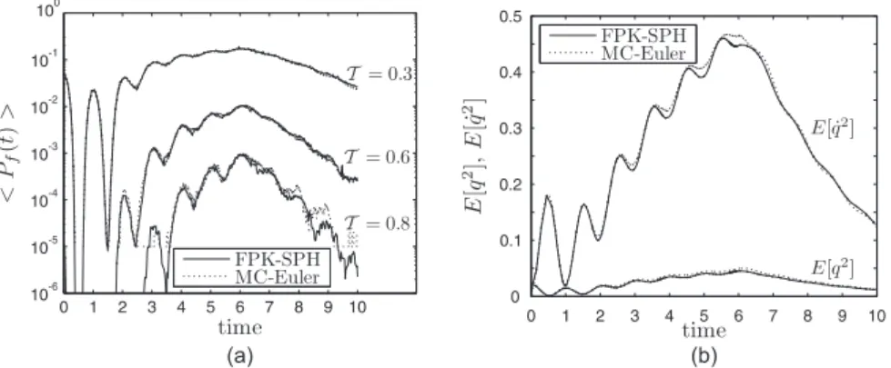
Figure 1: SDOF system with nonlinear viscous damper (Np= 1650). The probability of exceedance Pf(a) for the
system (26) is estimated for different thresholdsT . The results obtained by solving FPK with SPH are compared with Monte-Carlo (MC) simulations (105samples). The estimated second-order moments of q and ˙q are compared
with simulations (b) .
Figure 1-a shows < Pf > for different thresholds T calculated with FPK equation and
Eq.(25). These results are compared with Monte-Carlo simulations (105 samples and 216time
steps). For the Monte-Carlo method, Eq.(26) is integrated with a forward Euler scheme [4]. This figure shows the good agreement between results obtained with both methods, especially for high probabilities of exceedance. As expected, the convergence of stochastic simulations for low probabilities (in the order of 10−4) is not achieved. Because the response is not ergodic, a larger number of simulations is required to obtain accurate results. However, the computation of FPK equation has required about 11000 adaptive time steps and a single simulation has covered six orders of magnitude. Figure 1-b shows the estimation of the second-order moments of q and
˙
q estimated with Eq.(21) and highlights the ability of the method to capture the oscillations of the moments (and therefore in the system response). Some small differences with simulation results are observed, but the second-order moments of q and ˙q are properly estimated, despite an order of magnitude of difference between them, because the pdf is more stretched in the ˙q direction than in the q direction.
4.2 Probability of exceedance of a hysteretic oscillator
As another application, an SDOF system presenting a nonlinear elastoplastic behaviour and subjected to a transient seismic loading is considered. This example shows that the proposed method gives accurate information about the tail distribution through a reliability problem.
The equations of motion for a second-order structural system with hysteretic behavior are ¨ q + 2ξω0q + Φ = a˙ ⋆W Φ = ω2 0(αq + (1− α)z) ˙z = ˙q (A− (βsign( ˙qz) + γ) |z|n) (28) with q the dimensionless coordinate of the SDOF system, ξ the structural damping ratio and ω0 the natural circular frequency. The excitation is a white noise W (t) (E[W (t)W (t + τ )] =
2S0δ(τ )) modulated by a time window a⋆(t), while Φ(q, z) is the elastoplastic restoring force.
This force is a convex combination of a linear stiffness component and a hysteretic component depending on the hardening parameter α. The hysteretic behavior is controlled by the Bouc-Wen model characterized by the dimensionless variable z gathering the loading history and by the four parameters A, γ, β and n [30]. The outcome space is defined as ΩT ={q ∈ R : |q| > T > 0} for different values for the threshold T .
In this example, the parameters of the system are chosen as ω0 = π, ξ = 5%, α = 0.5 and
S0 = 1.0 and those of the Bouc-Wen model are A = 1, γ = 0.5, β = 0.5, n = 1. This set of
data provides a significantly nonlinear response. The time window is chosen as a⋆(t) = fmax t tmax exp ( 1− t tmax ) (29) with tmax = 2 and fmax = 1. The initial uncorrelated Gaussian distribution is slightly dispersed
with standard deviations equal to 0.05 and means equal to zero for q, ˙q and z. The number of particles is 9261 (=213) and the Courant number is 0.8. Initially, particles are regularly arranged
in a cube with an edge size of 0.4, and thus with 21 particles along each dimension.
Figure 2: (a) Probability density function ψ of the elastoplastic oscillator calculated with 9261 particles at time
t = 3.6 corresponding to the maximum variance. The darker the larger pdf, the lighter the lower pdf. Side
and bottom views are projections on lateral faces; they illustrate the saturation effect on z ∈ [−1; 1] although the solution space isR3. (b) Probability of exceedance Pf for system (28) estimated for different thresholdsT .
Results obtained with SPH are compared with Monte-Carlo (MC) simulations (5· 105samples).
This example shows in a three-dimensional state space that information about the tail distri-bution is accurately obtained with a reasonable number of particles and a number of time steps limited to 35000. With only one run, the proposed method covers six orders of magnitude in the probability of exceedance, see Fig. 2-b, whilst the Monte Carlo simulation, presented here with 5· 105runs, poorly estimates probabilities lower than 10−5. It would require approximately 108 runs to capture probabilities less than 10−5.
Besides this apparent robustness regarding the adaptation of the particle field from initial to transient states, the SPH algorithm proves to be efficient in containing the particles in the authorized subspace of the response domain. Indeed, the history variable z in this model is known to be limited to z ∈ [−A; A], as illustrated in Figure 2-a. Although no specific boundary condition is imposed, i.e. particles are thus free the move in the state space according to the governing equations, the SPH algorithm contains particles in the subspace limited by planes z =±1, as shown by the S-shaped projection of the pdf in the (q, z) plane.
5 Conclusions
In this paper, a contribution in the topic of the resolution of FPK equation with SPH method has been exposed. Some results in two and three dimensions are shown to illustrate the relevance of the proposed developments and assumptions. To conclude, some advantages and limitations are objectively summarized.
The Lagrangian formalism makes the method robust to deal with a large range of initial conditions even very different from the steady-state distribution. Only an accurate representa-tion of the initial condirepresenta-tion (even slightly dispersed) must be worried about. Furthermore, the implemented SPH method ensures the positivity of the pdf.
Nevertheless, the method has also some limitations. For instance, the stationary distribution cannot be directly computed which makes it more suited to transient problems. In the context of extreme value problems, the SPH method is limited because particles are not necessary located in low density zones. From a computational point of view, for a large number of particles, the computation of the interaction can turn out to be time consuming and the recourse to advanced cell mapping or sorting algorithm could be mandatory.
Although being mainly exploratory, this work throws light on a new possible use of the SPH method. As presented in this paper, the method offers already the possibility to rapidly and easily extend the formalism to multidimensional spaces and to have an accurate representation of the transient regime of the FPK equation.
Acknowledgment
The authors would like to acknowledge the National Fund for Scientific Research of Belgium for its support.
REFERENCES
[1] Y.K. Lin and G.Q. Cai. Probabilistic Structural Dynamics. Advanced Theory and Appli-cations. McGraw-Hill, New-York, 2nd edition, 2004.
[2] B. Oksendal. Stochastic differential equations. Springer-Verlag, 3rd edition, 1992. [3] H. Risken. The Fokker-Planck Equation. Methods of solution and applications.
Springer-Verlag, 2nd edition, 1996.
[4] D.P. Kroese, T. Taimre, and Z.I. Botev. Handbook of Monte Carlo Methods. Wiley series in probability and statistics, 2011.
[5] M. Grigoriu. Stochastic Calculus. Applications in Science and Engineering. Birkhauser, Boston, 1st edition, 2002.
[6] C. Soize. Steady-state solution of Fokker-Planck equation in high dimension. Probabilistic Engineering Mechanics, 3(4):196–206, 1988.
[7] J. S. Chang and G. Cooper. A practical difference scheme for Fokker-Planck equations. Journal of Computational Physics, 6:1–16, 1970.
[8] B.F. Spencer and L.A. Bergman. On the numerical solution of the Fokker-Planck equation for nonlinear stochastic systems. Nonlinear Dynamics, 4:357–372, 1993.
[9] A. Lozinski and C. Chauvii`ere. A fast solver for Fokker-Planck equation applied to viscoelastic flows calculations: 2d fene model. Journal of Computational Physics, 189(2):607–625, 2003.
[10] C. Chauvi`ere and A. Lozinski. Simulation of dilute polymer solutions using a Fokker-Planck equation. Computers & Fluids, 33(5-6):687–696, 2004.
[11] F. Chinesta, G. Chaidron, and A. Poitou. On the solution of Fokker-Planck equations in steady recirculating flows involving short fiber suspensions. Journal of Non-Newtonian Fluid Mechanics, 113(2-3):97–125, 2003.
[12] A. Ammar, B. Mokdad, F. Chinesta, and R. Keunings. A new family of solvers for some classes of multidimensional partial differential equations encountered in kinetic theory modeling of complex fluids. Journal of Non-Newtonian Fluid Mechanics, 139(3):153– 176, 2006.
[13] A. Ammar, B. Mokdad, F. Chinesta, and R. Keunings. A new family of solvers for some classes of multidimensional partial differential equations encountered in kinetic theory modelling of complex fluids: Part II: Transient simulation using space-time separated representations. Journal of Non-Newtonian Fluid Mechanics, 144(2-3):98–121, 2007. [14] L. Chupin. Fokker-Planck equation in bounded domain. Annales de l’Institut Fourier,
60(1), 2010.
[15] A. Der Kiureghian. Structural reliability methods for seismic safety assessment: a review. Engineering Structures, 18(6):412–424, 1996.
[16] L. B. Lucy. A numerical approach to the testing of the fission hypothesis. Astronomical Journal, 82:1013–1024, 1977.
[17] J. Feldman and J. Bonet. Dynamical refinement and boundary contact forces in SPH with applications in fluid flow problems. International Journal for Numerical Methods in Engineering, 72:295–324, 2007.
[18] T. Rabczuk and T. Belytschko. A three-dimensional large deformation meshfree method for arbitrary evolving cracks. Computer Methods in Applied Mechanics and Engineering, 196(29-30):2777–2799, 2007.
[19] G. R. Johnson, R. A. Stryk, and S. R. Beissel. SPH for high velocity impact computations. Computer Methods in Applied Mechanics and Engineering, 139(1-4):347–373, 1996. [20] P.W. Cleary and J.J. Monaghan. Conduction modelling using Smoothed particle
hydrody-namics. Journal of Computational Physics, 148:227–264, 1999.
[21] P. W. Randles and L. D. Libersky. Smoothed particle hydrodynamics: Some recent im-provements and applications. Computer Methods in Applied Mechanics and Engineering, 139:375–408, 1996.
[22] J. J. Monaghan. Smoothed particle hydrodynamics. Reports on Progress in Physics, 68:1703–1759, 2005.
[23] G.R. Liu and M.B. Liu. Smoothed Particle Hydrodynamics. A meshfree particle method. World Scientific Publ., 2003.
[24] C.V. Chaubal, A. Srinivasan, O. Egecioglu, and L.G. van Leal. Smoothed particle hy-drodynamics techniques for the solution of kinetic theory problems. Journal of Non-Newtonian Fluid Mechanics, 70:125–154, 1997.
[25] A. Ammar and F. Chinesta. A Particle Strategy for Solving the Fokker-Planck Equa-tion Modelling the Fiber OrientaEqua-tion DistribuEqua-tion in Steady Recirculating Flows Involv-ing Short Fiber Suspensions - Meshfree Methods for Partial Differential Equations II, vol-ume 43 of Lecture Notes in Computational Science and Engineering, pages 1–15. Springer Berlin Heidelberg, 2005.
[26] G. Lacombe. Analyse d’une ´equation de vitesse de diffusion. Comptes rendus de l’Acad´emie des sciences, Math., 329:383–386, 1999.
[27] T. Canor and V. Deno¨el. Transient Fokker-Planck equation solved with smoothed particle hydrodynamics method. Internation Journal of Numerical Methods in Engineering, 2013. DOI : 10.1002/nme.4461.
[28] M. Di Paola, L. Mendola, and G. Navarra. Stochastic seismic analysis of structures with nonlinear viscous dampers. Journal of Structural Engineering, 133(10):1475–1478, 2007. [29] G. Pekcan, J. B. Mander, and S. S. Chen. Fundamental considerations for the de-sign of non-linear viscous dampers. Earthquake Engineering and Structural Dynamics, 28(11):1405–1425, 1999.
[30] M. Ismail, F. Ikhouane, and J. Rodellar. The hysteresis Bouc-Wen model, a Survey. Archives of Computational Methods in Engineering, 16(2):161–188, 2009.