HAL Id: inria-00558509
https://hal.inria.fr/inria-00558509v2
Submitted on 12 Apr 2011
HAL is a multi-disciplinary open access
archive for the deposit and dissemination of
sci-entific research documents, whether they are
pub-lished or not. The documents may come from
teaching and research institutions in France or
L’archive ouverte pluridisciplinaire HAL, est
destinée au dépôt et à la diffusion de documents
scientifiques de niveau recherche, publiés ou non,
émanant des établissements d’enseignement et de
recherche français ou étrangers, des laboratoires
Florian Brandner, Benoit Boissinot, Alain Darte, Benoît Dupont de Dinechin,
Fabrice Rastello
To cite this version:
Florian Brandner, Benoit Boissinot, Alain Darte, Benoît Dupont de Dinechin, Fabrice Rastello.
Com-puting Liveness Sets for SSA-Form Programs. [Research Report] RR-7503, INRIA. 2011, pp.25.
�inria-00558509v2�
a p p o r t
d e r e c h e r c h e
ISRN
INRIA/RR--7503--FR+ENG
Domaine 2
Computing Liveness Sets for SSA-Form Programs
Florian Brandner — Benoit Boissinot — Alain Darte — Benoît Dupont de Dinechin —
Fabrice Rastello
N° 7503 — version 2
Florian Brandner
∗, Benoit Boissinot
∗, Alain Darte
∗,
Benoît Dupont de Dinechin
†, Fabrice Rastello
∗ Domaine : Algorithmique, programmation, logiciels et architecturesÉquipe-Projet COMPSYS
Rapport de recherche n° 7503 — version 2 — initial version Janvier 2011 — revised version Avril 2011 — 25 pages
Abstract: We revisit the problem of computing liveness sets, i.e., the set of variables live-in and live-out of basic blocks, for programs in strict SSA (static single assignment). Strict SSA is also known as SSA with dominance property because it ensures that the definition of a variable always dominates all its uses. This property can be exploited to optimize the computation of liveness sets.
Our first contribution is the design of a fast data-flow algorithm, which, unlike traditional approaches, avoids the iterative calculation of a fixed point. Thanks to the properties of strict SSA form and the use of a loop-nesting forest, we show that two passes are sufficient. A first pass, similar to the initialization of iterative data-flow analysis, traverses the control-flow graph in postorder propagating liveness information backwards. A second pass then traverses the loop-nesting forest, updating liveness information within loops.
Another approach is to propagate from uses to definition, one variable and one path at a time, instead of unioning sets as in standard data-flow analysis. Such a path-exploration strategy was proposed by Appel in his “Tiger book” and is also used in the LLVM compiler. Our second contribution is to show how to extend and optimize algorithms based on this idea to compute liveness sets one variable at a time using adequate data structures.
Finally, we evaluate and compare the efficiency of the proposed algorithms using the SPECINT 2000 benchmark suite. The standard data-flow approach is clearly outperformed, all algorithms show substantial speed-ups of a factor of 2 on average. Depending on the underlying set implementation either the path-exploration approach or the loop-forest-based approach provides superior performance. Experiments show that our loop-forest-based algorithm provides superior performances (average speed-up of 43% on the fastest alternative) when sets are represented as bitsets and for optimized programs, i.e., when there are more variables and larger live-sets and live-ranges.
Key-words: Liveness Analysis, SSA form, Compilers
This work is partly supported by the compilation group of STMicroelectronics.
∗Compsys, LIP, UMR 5668 CNRS, INRIA, ENS-Lyon, UCB-Lyon †Kalray
Résumé :
Nous réexaminons le problème du calcul des ensembles de vivacité, c’est-à-dire des ensembles de variables en vie en entrée et sortie des blocs de base d’un programme en forme SSA (assignation unique statique) stricte. La forme SSA stricte est également appelée SSA avec propriété de dominance parce qu’elle garantit que la définition d’une variable domine toujours toutes ses utilisations. Nous exploitons cette propriété pour optimiser le calcul de vivacité.
Notre première contribution est la conception d’un algorithme rapide de type flot de données qui, à la différence des approches traditionnelles, évite les itérations de calcul de point fixe. Grâce aux propriétés de la forme SSA stricte et à l’utilisation d’une hiérarchie de boucles (“loop-nesting forest”), nous montrons que deux passes sont suffisantes. Une première passe, similaire à la phase d’initialisation de la méthode de flot de données itérative, propage les informations de vivacité en remontant un parcours en profondeur du graphe de flot de contrôle. Une deuxième passe parcourt la hiérarchie de boucles pour mettre à jour l’information dans les boucles.
Une autre approche consiste à propager depuis les utilisations jusqu’à la dé-finition, une variable et un chemin à la fois, plutôt que d’effectuer des unions d’ensembles comme dans l’analyse de flot de données standard. Une telle stra-tégie d’exploration des chemins a été proposée par Appel dans son “Tiger book” et est également utilisée dans le compilateur LLVM. Notre seconde contribu-tion est de montrer comment étendre et optimiser un algorithme basé sur cette idée pour calculer les ensembles de vivacité, une variable à la fois, et avec des structures de données adéquates.
Finalement, nous évaluons et comparons les performances des algorithmes proposés avec les “benchmarks” de SPECINT 2000. L’approche traditionnelle de flot de données est clairement surpassée par les autres algorithmes, avec un facteur d’amélioration de 2 en moyenne. Selon l’implantation des ensembles de vivacité, la meilleure approche est soit celle par remontée de chemin, soit celle utilisant la hiérarchie de boucles. Les expérimentations montrent que notre algorithme flot de données offre de meilleures performances (amélioration de 43% par rapport à la meilleure alternative) quant les ensembles sont représentés par des “bitsets” et pour les programmes optimisés, programmes avec plus de variables, et des ensembles de vivacité et des intervalles de vie plus grands. Mots-clés : Calcul des ensembles de vivacité, affectation unique statique, compilateur
1
Introduction
Static single assignment (SSA) form is a popular program representation used by most modern compilers today. Initially developed to facilitate the develop-ment of high-level program transformations, SSA form has gained much interest in the scientific community due to its favorable properties that often allow to simplify algorithms and reduce computational complexity. Today, SSA form is even adopted for the final code generation phase [22], i.e., the backend. Several industrial and academic compilers, static or just-in-time, use SSA in their back-ends, e.g., LLVM [24], Java HotSpot [21], LAO [13], LibFirm [23, 10], Mono [27]. Recent research on register allocation [6, 14, 29] even allows to retain SSA form until the very end of the code generation process.
This work investigates the use of SSA properties to simplify and acceler-ate liveness analysis, i.e., an analysis that determines for all variables the set of program points where the variables’ values are eventually used by subse-quent operations. Liveness information is essential to solve storage assignment problems, eliminate redundancies, and perform code motion. For instance, op-timizations like software pipelining, trace scheduling, register-sensitive redun-dancy elimination, if-conversion, as well as register allocation heavily rely on liveness information.
Traditionally, liveness information is obtained by data-flow analysis: liveness sets are computed for all basic blocks and variables in parallel by solving a set of data-flow equations [3]. These equations are usually solved by an iterative algorithm, propagating information backwards through the control-flow graph (CFG) until a fixed point is reached and the liveness sets stabilize. The number of iterations depends on the control-flow structure of the considered program, more precisely on the structure of its loops.
In this paper, we show that, for SSA-form programs, it is possible to design a data-flow algorithm to compute liveness sets that does not require to iterate to reach a fixed point. Instead, at most two passes over the CFG are necessary. The first pass, very similar to traditional data-flow analysis, computes partial liveness sets by traversing the CFG backwards. The second pass refines the partial liveness sets and computes the final solution by traversing a loop-nesting forest, as defined by Ramalingam [31]. For the sake of clarity, we first present our algorithm for reducible CFGs. Irreducible CFGs can be handled with a slight variation of the algorithm, with no need to modify the CFG itself (Section 4.3). Since our algorithm exploits advanced program properties some prerequisites have to be met by the input program and the compiler framework:
• The CFG of the input program is available. • The program has to be in strict SSA form. • A loop-nesting forest of the CFG is available.
These assumptions are weak and easy to meet for clean-sheet designs. The SSA requirement is the main obstacle for compilers not already featuring it.
For SSA programs, another approach is possible that follows the classical definition of liveness: a variable is live at a program point p, if p belongs to a path of the CFG leading from a definition of that variable to one of its uses without passing through another definition of the same variable. Therefore, the live-range of a variable can be computed using a backward traversal starting on its uses and stopping when reaching its (unique) definition. For comparison, we designed optimized implementations of this path-exploration principle (see
Section 5), for both SSA and non-SSA programs, and compared the efficiency of the resulting algorithms with our novel non-iterative data-flow algorithm.
Our experiments using the SPECINT 2000 benchmark suite in a production compiler demonstrate that the non-iterative data-flow algorithm outperforms the standard iterative data-flow algorithm by a factor of 2 on average. By construction, our algorithm is best suited for a set representation, such as bitsets, favoring operations on whole sets. In particular, for optimized programs, which have non-trivial live-ranges and a larger number of variables, our algorithm achieves a speed-up of 43% on average in comparison to the fastest alternative based on path exploration.
Before detailing our two-passes data-flow algorithm (Section 4) and the al-gorithms based on path-exploration (Section 5), we summarize in Section 2 different approaches for liveness analysis and provide in Section 3 some con-cepts that form the theoretical underpinning of our algorithm. Experiments are described in Section 6. We conclude in Section 7.
2
Related Work
Literature treating specifically the problem of liveness computation is rare. The general approach is to use iterative data-flow analysis, which goes back to Kil-dall [20]. The algorithms are, however, not specialized to the computation of liveness sets, and may thus incur overhead. Kam et al. [19] explored the com-plexity of round-robin data-flow algorithms, i.e., those propagating information according to a node ordering derived from a depth-first spanning tree T and it-erating until the analysis result stabilizes. Generalizing the result of Hecht and Ullman [17], they showed that the number of iterations for data-flow problems on graphs is bounded by d(G, T ) + 3, where d(G, T ) denotes the loop connect-edness of the (reverse) control-flow graph G for T , i.e., the maximal number of back edges (with respect to T ) in a cycle-free path in G (see also Section 4). Empirical results by Cooper [11] indicate that the order in which basic blocks are processed is critical and directly impacts the number of iterations. In con-trast, our non-iterative data-flow algorithm requires at most two passes over the CFG, in all cases.
An alternative way to solve data-flow problems is interval analysis [2] and other elimination-based approaches [32]. The initial work on interval analysis [2] demonstrates how to compute liveness information using only three passes over the intervals of the CFG. However, the problem statement involves, besides the computation of liveness sets, several intermediate problems, including separate sets for reaching definitions and upward-exposed uses. Furthermore, the num-ber of intervals of a CFG grows with the numnum-ber of loops. Also, except for the Graham-Wegman algorithm, interval-based algorithms require the CFG (resp. the reverse CFG) to be reducible for a forward (resp. backward) analysis [32]. In practice, irreducible CFGs are rare, but liveness analysis is a backward data-flow problem, which frequently leads to irreducible reverse CFGs. In contrast, our algorithm does not require the reverse CFG to be reducible. However, if the CFG is irreducible, the backward traversal of the CFG (and the corre-sponding propagation of liveness information) needs to be slightly modified (see Section 4.3), but with no modification of the CFG itself.
Another approach to compute liveness was proposed by Appel [3, p. 429]. Instead of computing the liveness information for all variables at the same time,
variables are handled individually by exploring paths through the CFG start-ing from variable uses. An equivalent approach usstart-ing logic programmstart-ing was presented by McAllester [25], showing that liveness analysis can be performed in time proportional to the number of instructions and variables of the input program. However, his theoretical analysis is limited to an input language with simple conditional branches having at most two successors. A more generalized analysis will be given later, both in terms of theoretical complexity (Section 5.4) and of practical evaluation (Section 6).
3
Foundations
This section introduces the notations used throughout this paper and presents the necessary theoretical foundations. Readers familiar with flow graphs, loop-nesting forests, dominance, and SSA form can skip ahead to Section 4.
3.1
Control Flow and Loop Structure
A control-flow graph G = (V, E, r) is a directed graph, with nodes V , edges E, and a distinguished node r ∈ V with no incoming edges. Usually, the CFG nodes represent the basic blocks of a procedure or function, every block is in turn associated with a list of operations or instructions.
PathsLet G = (V, E, r) be a CFG. A path P of length k from a node u to a node v in G is a non-empty sequence of nodes (v0, v1, . . . , vk) such that
u = v0, v = vk, and (vi−1, vi) ∈ Efor i ∈ [1..k]. Implicitly, a single node forms
a (trivial) path of length 0 and a self-loop forms a path of length 1. We assume that the CFG is connected, i.e., there exists a path from the root node r to every other node.
DominanceA node x in a CFG dominates another node y if every path from the root r to y contains x. The dominance is said to be strict if, in addition, x 6= y. A well-known property is that the transitive reduction of the dominance relation forms a tree, the dominator tree.
Loop-nesting forestRamalingam [31] gave a recursive constructive defi-nition of loop-nesting forests as follows:
1. Partition the CFG into its strongly connected components (SCCs). Every non-trivial SCC, i.e., with at least one edge, is called a loop.
2. Within each non-trivial SCC, consider the set of nodes not dominated by any other node of the same SCC. Among these nodes, choose a non-empty subset and call it the set of loop-headers.
3. Remove all edges, inside the SCC, that lead to one of the loop-headers. Call these edges the loop-edges.
4. Repeat this partitioning recursively for every SCC after removing its loop-edges. The process stops when only trivial SCCs remain.
This decomposition can be represented by a forest, where each non-trivial SCC, i.e., every loop, is represented by an internal node. The children of a loop’s node represent all inner loops (i.e., all non-trivial SCCs it contains) as well as the regular basic blocks of the loop’s body. The forest can easily be turned into a tree by introducing an artificial root node, corresponding to the entire CFG. Its leaves are the nodes of the CFG, while internal nodes, labeled by loop-headers, correspond to loops. Note also that a loop-header cannot belong
to any inner loop because all edges leading to it are removed before computing inner loops.
Reducible control-flow graphs A CFG is reducible if every loop has a single loop-header that dominates all nodes of the loop [16]. In other words, the only way to enter a loop is through its unique loop-header. Because of its structural properties, the class of reducible control-flow graphs is of special interest for compiler writers. Indeed, the vast majority of programs exhibit reducible CFGs. Also, as pointed out earlier, unlike other approaches that compute liveness information, we only need to discuss the reducibility of the original CFG, not of the reverse CFG.
Computing a loop-nesting forestThe loop-nesting forest of a reducible CFG is unique and can be computed in O(|V | log∗(|E|)). For example, Tarjan’s
algorithm [34] performs a bottom up traversal in a depth-first search tree of the CFG, identifying inner (nested) loops first. Because irreducible loops have more than one undominated node, the loop-nesting forest of an irreducible graph is not unique [31]. An interesting and simple-to-engineer loop-nesting forest algorithm is the one of Havlak [15], later improved by Ramalingam [30] to fix a complexity issue. Havlak’s algorithm is a simple generalization of Tarjan’s algorithm. It identifies a loop as a set of descendants of a back-edge target that can reach its source. In that case, the set of loop-headers is restricted to a single entry node, the target of a back-edge. Also, during the process of loop identification, whenever an entry node that is not the loop-header is encountered, the corresponding incoming edge (from a non-descendant node) is replaced by an edge to the loop-header.
3.2
Static Single Assignment Form
Static single assignment (SSA) form [12], is a popular program representation used in many compilers nowadays. In SSA form, each scalar variable is defined only once statically in the program text. To construct SSA form, variables hav-ing multiple definitions are replaced by several new SSA-variables, one for each definition. A problem appears when a use in the original program was reach-able from multiple definitions. The new varireach-ables need to be disambiguated in order to preserve the program’s semantic. The problem is solved by introducing φ-functions that are placed at control-flow joins. Depending on the actual execu-tion flow, a φ-funcexecu-tion defines a new SSA-variable by selecting the SSA-variable corresponding to the respective definition.
In this paper, we require that the program under SSA form is strict. In a strict program, every path from the root r to a use of a variable contains the definition of this variable. Because there is only one (static) definition per variable, strictness is equivalent to the dominance property, which states that each use of a variable is dominated by its definition. This is true for all uses including a use in a φ-operation by considering that such a use actually takes place in the predecessor block from where it originates.
3.3
Liveness
Liveness is a property relating program points to sets of variables which are considered to be live at these program points. Intuitively, a variable is con-sidered live at a given program point when its value is used in the future by
any dynamic execution. Statically, liveness can be approximated by following paths, backwards, through the control-flow graph leading from uses of a given variable to its definitions - or in the case of SSA form to its unique definition. The variable is live at all program points along these paths. For a CFG node q, representing an instruction or a basic block, a variable v is live-in at q if there is a path, not containing the definition of v, from q to a node where v is used. It is live-out at q if it is live-in at some successor of q.
The computation of live-in and live-out sets at the entry and the exit of basic blocks is usually termed liveness analysis. It is indeed sufficient to consider only these sets since liveness within a basic block is trivial to recompute from its live-out set, either by traversing the block or by precomputing which variables are defined or upward-exposed (see Section 4). Live-ranges are closely related to liveness. Instead of associating program points with sets of live variables, the live-range of a variable specifies the set of program points where that variable is live. Live-ranges in programs under strict SSA form exhibit certain useful properties, some of which have been exploited for register allocation [14, 6], some of which can be exploited during the computation of liveness information. However, the special behavior of φ-operations often causes confusion on where exactly its operands are actually used and defined.
For a regular operation, variables are used and defined where the operation takes place. However, the semantics of φ-functions (and in particular the actual place of φ-uses) should be defined carefully, especially when dealing with SSA destruction. In all algorithms for SSA destruction, such as [7, 33, 5], a use in a φ-operation is considered live somewhere inside the corresponding predecessor block, but, depending on the algorithm and, in particular, the way parallel copies are inserted, it may or may not be considered as live-out for that predecessor block. Similarly, the definition of a φ-operation is always considered to be at the beginning of the block, but, depending on the algorithm, it may or may not be marked as live-in for the block. To make the description of algorithms easier, we follow the definition by Sreedhar [33]. For a φ-function a0 = φ(a1, . . . , an)
in block B0, where ai comes from block Bi, then:
• a0 is considered to be live-in for B0, but, with respect to this φ-function,
it is not live-out for Bi, i > 0.
• ai, i > 0, is considered to be live-out of Bi, but, with respect to this
φ-function, it is not live-in for B0.
This corresponds to placing a copy of ai to a0 on each edge from Bi to B0.
The data-flow equations given hereafter and the presented algorithms follow the same semantics. They require minor modifications when other φ-semantics are desired. We will come back to these subtleties in Section 4.2.2.
3.4
Complexity of Liveness Algorithms
The running times of liveness algorithms depend on several parameters. Some of them can only be evaluated by experiments, for example the locality in data structures, the cost of function calls instead of inlined operations, etc. This will be discussed in Section 6. However, some of them can be evaluated statically:
• How often are the program’s instructions visited? • How often are the CFG edges and nodes traversed?
• How many operations are performed on the algorithm’s data structures and how costly are they?
Usually, liveness algorithms do not consider local variables, i.e., those defined in a block and used only there, as they are not part of live-in and live-out sets. The complexity of operations on variable sets is then measured in terms of |W |, where W is the set of non-local variables, called global variables. However, to identify local and global variables, to identify uses and definitions, all instruc-tions of the program P need to be visited. Traversing its internal representation is costly and, moreover, is not necessarily linked to |W | as it involves all vari-ables. In other words, any liveness algorithm requires at least |P | operations to read the program and, in practice, it is better to read it only once.
After possibly some precomputations in O(|P |) operations, liveness algo-rithms work on the CFG G = (V, E, r). The number of operations can then be evaluated in terms of |V | and |E|, i.e., the number of times blocks and control-flow edges are visited. Hereafter, we assume |V | − 1 ≤ |E| ≤ |V |2. The costs
of these operations depend on the data structures used, both for intermediate results (e.g., uses of a variable or upward-exposed uses in a block) and for the final results, the live-in and live-out sets. For these sets, either lists (ordered or unordered) or bitsets can be used (we will not consider hash tables). The com-plexity has then to be discussed according to the operations performed: test if an element is in a set, insertion in a set, union of two sets, sorting of a set. The best choice of the data structures may depend on the liveness algorithm used, but also on the algorithms that will use the live-in and live-out sets afterwards. Such a complexity analysis will be done for each algorithm given hereafter.
4
Data-Flow Approaches
A well-known and frequently used approach to compute the live-in and live-out sets of basic blocks is backward data-flow analysis [3]. The liveness sets are given by a set of equations that relate the upward-exposed uses and the definitions occurring within a basic block to the live-in and live-out sets of the predecessors and successors in the CFG. A use is said to be upward-exposed when a variable is used within a basic block and no definition of the same variable precedes the use locally within that basic block. The sets of upward-exposed uses and definitions do not change during liveness analysis and can thus be precomputed. In the following equations, we denote by PhiDefs(B) the variables defined by φ-operations at entry of the block B and by PhiUses(B) the set of variables used in a φ-operation at entry of a block successor of the block B.
LiveIn(B) = PhiDefs(B) ∪ UpwardExposed(B) ∪ (LiveOut(B) \ Defs(B)) LiveOut(B) = SS∈succs(B)(LiveIn(S) \ PhiDefs(S)) ∪ PhiUses(B)
4.1
Complexity of Standard Data-Flow Approaches
The equations of the data-flow analysis can be solved efficiently using a simple iterative work-list algorithm that propagates liveness information among the basic blocks of the CFG. The liveness sets are refined on every iteration of the algorithm until a fixed point is reached, i.e., the algorithm stops when the sets cannot be refined any further. When the work-list contains edges of the CFG, the number of set operations can be bounded by O(|E||W |) [28], as each set can be modified (grow) at most |W | times. As recalled in Section 2, the round robin algorithm [17, 19] allows another bound to be derived based on d(G, T ), the loop
connectedness of the reverse CFG G, i.e., the maximal number of back edges (with respect to a depth-first spanning tree T ) in a cycle-free path in G. The algorithm traverses the complete CFG on every iteration, at most (d(G, T ) + 3) times, and thus results in O(|E|(d(G, T ) + 3)) set operations. These operations are mainly unions of sets, which can be performed in O(|W |) for bitsets or ordered lists. The complexity is higher for unordered lists as the union is more costly, unless an intermediate sparse-set is used [8].
Depending on the structure of the program being analyzed, either of the two algorithms leads to a faster termination. In addition, both need a preliminary step to compute the upward-exposed uses and definitions of each basic block. This requires visiting every instruction of the program once, thus in time O(|P |) where |P | is the size of the program representation. Each operation consists in possibly inserting a global variable in a set, which is O(1) for a bitset, O(log(|W |) for an ordered list, and O(|W |) for an unordered list. For this last case, it is only O(1) if a flag for each variable attests that the variable has not been already inserted, as it is for example done in Algorithm 8. Finally, assuming that the insertion is indeed O(1), thus in particular for bitsets, the overall complexity is either O(|P | + |E||W |2) or O(|P | + |E||W |(d(G, T ) + 3)) depending on the
update strategy. Our contribution in the rest of this section is the design, for strict SSA programs, of a liveness data-flow algorithm whose complexity is only O(|P | + |E||W |), in other words, near-optimal as it includes the time to read the program, i.e., O(|P |), and the time to propagate/generate the output, i.e., O(|E||W |). We point out that it is also possible to design optimized algorithms based on path exploration, with the same near-optimal complexity O(|P | + |E||W |), and operating at basic block level. This will be explained in Section 5.
4.2
Liveness Sets On Reducible Graphs
Instead of computing a fixed point, we show that liveness information can be derived in two passes over the control-flow graph by exploiting properties of strict SSA form. The first version of the algorithm requires the CFG to be reducible. We then show that arbitrary control-flow graphs can be handled elegantly and with no additional cost, except for a cheap preprocessing step on the loop-nesting forest. The algorithm proceeds in two steps:
1. A backward pass propagates partial liveness information upwards using a postorder traversal of the CFG.
2. The partial liveness sets are then refined by traversing the loop-nesting forest, propagating liveness from loop-headers down to all basic blocks within loops.
Algorithm 1 shows the necessary initialization and the high-level structure to compute liveness in two-passes.
Algorithm 1 Two-passes liveness analysis: reducible CFG. 1: function Compute_LiveSets_SSA_Reducible(CFG) 2: foreach basic block B do
3: mark B as unprocessed
4: DAG_DFS(R) . Ris the CFG root node
5: foreach root node L of the loop-nesting forest do 6: LoopTree_DFS(L)
The postorder traversal is shown by Algorithm 2 which performs a simple depth-first search and associates every basic block of the CFG with partial live-ness sets. The algorithm roughly corresponds to the precomputation step of the traditional iterative data-flow analysis. However, loop-edges are not con-sidered during the traversal (Line 2). Recalling the definition of liveness for φ-operations, PhiUses(B) denotes the set of variables live-out of basic block B due to uses by φ-operations in B’s successors. Similarly, PhiDefs(B) denotes the set of variables defined by a φ-operation in B.
Algorithm 2 Partial liveness, with postorder traversal 1: function DAG_DFS(block B)
2: foreach S ∈ succs(B) if (B, S) is not a loop-edge do 3: if S is unprocessed then DAG_DFS(S)
4: Live =PhiUses(B)
5: foreach S ∈ succs(B) if (B, S) is not a loop-edge do 6: Live = Live ∪ (LiveIn(S) \ PhiDefs(S))
7: LiveOut(B) = Live
8: foreach program point p in B, backward do 9: remove variables defined at p from Live 10: add uses at p to Live
11: LiveIn(B) = Live ∪ PhiDefs(B) 12: mark B as processed
The next phase, traversing the loop-nesting forest, is shown by Algorithm 3. The live-in and live-out sets of all basic blocks within a loop are unified with the liveness sets of its loop-header. This is sufficient in order to compute valid liveness information due to the fact that a variable whose live-range crosses a back-edge of the loop is live-in and live-out at all basic blocks of the loop (see the proofs in Section 4.2.2).
Algorithm 3 Propagate live variables within loop bodies. 1: function LoopTree_DFS(node N of the loop forest) 2: if N is a loop node then
3: Let BN = Block(N ) .The loop-header of N
4: Let LiveLoop = LiveIn(BN) \PhiDefs(BN)
5: foreach M ∈ LoopTree_succs(N) do
6: Let BM = Block(M ) . Loop-header or block
7: LiveIn(BM) =LiveIn(BM) ∪ LiveLoop
8: LiveOut(BM) =LiveOut(BM) ∪ LiveLoop
9: LoopTree_DFS(M)
4.2.1 Complexity
In contrast to iterative data-flow algorithms, our algorithm has only two phases. The first traverses the CFG once, the second traverses the loop-nesting forest once. The number of operations performed during the CFG traversal of Algo-rithm 2 can be bounded by O(|V |+|E|) unions of sets and O(|P |) set insertions. Thus, assuming |V |−1 ≤ |E|, the complexity of the first phase is O(|E||W |+|P |) for bitsets. It is O(|E||W | + |P | log(|W |)) if ordered lists are used instead.
The traversal of the loop-nesting forest follows a similar pattern. The size of the forest is at most twice the number of basic blocks |V | in the CFG, because every loop node in the loop-nesting forest has one child node representing a basic block (a leaf in the forest). The loop body is executed exactly once for every node of the loop nesting forest, which gives an upper bound for the number of set (union) operations for Algorithm 3 in O(|V |). Since |V |−1 ≤ |E|, this phase does not change the overall complexity mentioned above. The same is true for the unmark initialization phase. Our non-iterative data-flow algorithm has thus the expected near-optimal complexity O(|P | + |E||W |), as claimed before. It avoids the multiplicative factor that bounds the number of iterations in standard iterative data-flow algorithms.
4.2.2 Correctness
The previous algorithms were specialized for the case where φ-functions are interpreted as parallel copies at the CFG edges preceding the φ-functions. For the correctness proofs, we resort to the following, more generic, φ-semantics. A φ-function a0 = φ(a1, . . . , an) at basic block B0, receiving its arguments from
blocks Bi, i > 0, is represented by a fresh variable aφ, a copy a0 = aφ at B0,
and copies aφ = ai at Bi, for i > 0. Now, with respect to this φ-function, ai,
for i > 0, is not live-out at Bi and a0 is not live-in at B0 anymore. As for aφ,
since it is not a SSA variable, it is not covered by the following lemmas. But its live-range is easily identified: it is live-in at B0 and live-out at Bi, i > 0,
and nowhere else. Other φ-semantics extend the live-ranges of the φ-operands with parts of the live-range of aφ and can thus be handled by locally refining
the live-in and live-out sets. This explains why, in Algorithm 2, PhiUses(B) is added to LiveOut(B) (Line 4), PhiDefs(B) is added to LiveIn(B) (Line 11), and PhiDefs(S) is removed from LiveIn(S) (Line 6). This ensures that the variable defined by a φ-function is marked as live-in and its uses as live-out at the predecessors. A similar adjustment appears on Line 4 of Algorithm 3.
The first pass propagates the liveness sets using a postorder traversal of the reduced graph FL(G) of the CFG, obtained by removing all loop-edges 1 from
the CFG. We first show that this pass correctly propagates liveness information to the loop-headers of the original CFG.
Lemma 1. Let G be a reducible CFG, v a SSA variable, and d its definition. If L is a maximal loop not containing d, then v is live-in at the loop-header h of L iff there is a path in FL(G), not containing d, from h to a use of v.
Proof. If v is live-in at h, there is a cycle-free path in the CFG from h to a use of v that does not go through d. Suppose this path contains a loop-edge (s, h0)
where h0 is the header of a loop L0, and s ∈ L0. Since the path has no cycle,
h06= h and thus L 6= L0. Now, two cases could occur:
• If h ∈ L0, L is contained in L0. As L is a maximal loop not containing
d, d ∈ L0. Thus h0 dominates d. This contradicts the fact that d strictly dominates all nodes where the variable v is live-in, in particular h0.
• If h 6∈ L0, then the path from h enters the loop L0a first time before going
through the loop-edge (s, h0). Since the graph is reducible, the only way
to enter L0 is through h0, thus there are two occurrences of h0 in the path.
Impossible since the path is cycle-free.
1Note that, since the CFG is reducible, the loop-forest is unique so there is no ambiguity
Thus, the path does not contain any loop-edges, which means that it is a valid path in FL(G). Conversely, if there exists a path in FL(G), then, of course, the
variable v is live-in at h, since FL(G)is a sub-graph of the original graph G.
Lemma 1 does not apply if there is no loop L satisfying the conditions. The following lemma covers this case.
Lemma 2. Let G be a reducible CFG, v a SSA variable, and d its definition. Let p be a node of G such that all loops containing p also contain d. Then v is live-in at p iff there is a path in FL(G), from p to a use of v, not containing d.
Proof. If v is live-in at p, there exists a cycle-free path in G from p to a use of v that does not contain d. Suppose this path contains a loop-edge (s, h) where h is the loop-header of a loop L, and s ∈ L:
• If p ∈ L then d ∈ L by hypothesis. Thus h dominates d, which is again, as in Lemma 1, impossible.
• If p 6∈ L, since s is in the loop, there has to be a previous occurrence of h on the path. Indeed, because the CFG is reducible, h is the only entry of L. This contradicts the fact that the path is cycle-free.
It follows that the path cannot contain any loop-edges. The path is thus a valid path in FL(G). Conversely, if there exists a path in FL(G), then v is live-in
at p, since FL(G) is a sub-graph of the original graph G.
Algorithm 2, which propagates liveness information along the DAG FL(G),
can only mark variables as live-in that are indeed live-in. Furthermore, if, after this propagation, a variable v is missing in the live-in set of a CFG node p, Lemma 2 shows that p belongs to a loop that does not contain the definition of v. Let L be such a maximal loop. According to Lemma 1, v is correctly marked as live-in at the header of L. The next lemma shows that the second pass of the algorithm (Algorithm 3) correctly adds variables to the live-in and live-out sets where they are missing.
Lemma 3. Let G be a reducible CFG, L a loop, and v a SSA variable. If v is live-in at the loop-header of L, it is live-in and live-out at every CFG node in L. Proof. If v is live-in at h, the loop-header of L, then the definition d of v strictly dominates the CFG node h, thus d 6∈ L. Indeed, h cannot be dominated by any other node in L. Let p be a CFG node in L. Since L is strongly connected, there is a non-trivial path from p to h. It does not contain d as d /∈ L. Since v is live-in at h, there is a path from h to a use of v that does not contain d. Concatenating these two paths proves that v is live-in at p. It is also live-out at p since p has a successor, where v is live-in, on the path from p to h.
This lemma proves the correctness of the second pass, which propagates the liveness information within loops. Every CFG node, which is not yet associated with accurate liveness information, is properly updated by the second pass. Moreover, no variable is added where it should not be added.
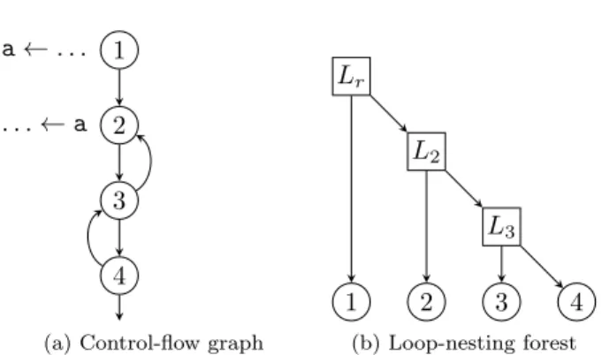
Example 1. The CFG of Figure 1a is a pathological case for iterative data-flow analysis. The precomputation phase does not mark variable a as live throughout the two loops. An iteration is required for every loop-nesting level until the final
1 a ← . . . 2 . . . ← a 3 4
(a) Control-flow graph
Lr L2 L3 4 3 2 1 (b) Loop-nesting forest Figure 1: Bad case for iterative data-flow analysis.
solution is computed. In our algorithm, after the CFG traversal, the traversal of the loop-nesting forest (Figure 1b) propagates the missing liveness information from the loop-header of loop L2down to all blocks within the loop’s body and
all inner loops, i.e., blocks 3 and 4 of L3.
4.3
Liveness Sets on Irreducible Flow Graphs
It is well-known that every irreducible CFG can be transformed into a semanti-cally equivalent reducible flow graph, for example, using node splitting [18, 1]. The graph may, unfortunately, grow exponentially during the processing [9]. However, when liveness information is to be computed, a relaxed notion of equivalence is sufficient. We first show that every irreducible CFG can be trans-formed into a reducible CFG, without size explosion, such that the liveness in both graphs is equivalent. Actually, there is no need to transform the graph explicitly. Instead, the effect of the transformation can be directly emulated in Algorithm 2, with a slight modification, so as to handle irreducible CFGs.
For every loop L, EntryEdges(L) denotes the set of entry-edges, i.e., the edges leading, from a basic block that is not part of the loop L, to a block within L. Entries(L)denotes the set of L’s entry-nodes, i.e., the nodes that are target of an entry-edge. Similarly, PreEntries(L) denotes the set of blocks that are the source of an entry-edge. The set of loop-edges is given by LoopEdges(L). Given a loop L from a graph G = (V, E, r), we define the graph ΨL(G) = (E0, V0, r)
as follows. The graph is extended by a new node δL, which represents the
(unique) loop-header of L after the transformation. All edges entering the loop from preentry-nodes are redirected to this new header. The loop-edges of L are similarly redirected to δL and additional edges are inserted leading from δL
to L’s former loop-headers. More formally:
E0 = E \ LoopEdges(L) \ EntryEdges(L) ∪ {(s, δL) | s ∈ PreEntries(L)}
∪{(s, δL) | ∃(s, h) ∈ LoopEdges(L)} ∪ {(δL, h) | h ∈ LoopHeaders(L)}
Repeatedly applying this transformation yields a reducible graph, slightly larger than the original graph, in which each node is still reachable from the root r. Depending on the order in which loops are considered, entry-edges may be up-dated several times during the processing in order to reach their final positions. But the loop-forest structure remains the same. The next example illustrates this transformation.
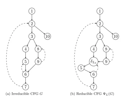
1 2 10 3 8 9 4 5 6 7 (a) Irreducible CFG G 1 2 10 3 8 9 4 δL5 5 6 7 (b) Reducible CFG ΨL(G)
Figure 2: A reducible CFG derived from an irreducible CFG, using the loop-forest depicted in Figure 3.
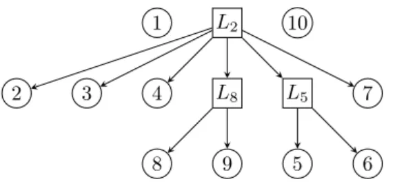
Example 2. Consider the CFG of Figure 2a and the loop-nesting forest in Fig-ure 3, where node 5 was selected as loop-header for L5, the loop containing the
nodes 5 and 6. As both nodes are entry-nodes, via the preentry-nodes 4 and 9, the CFG is irreducible. The transformed reducible graph ΨL5(G)is depicted in
Figure 2b. The graph might not reflect the semantics of the original program during execution, but it preserves the liveness properties of the original graph for a strict SSA program, as we will show in Theorem 1.
To avoid building this transformed graph explicitly, an elegant alternative is to modify the CFG traversal (Algorithm 2). To make things simpler, we assume that the loop forest is built so that, as in Havlak’s loop forest construction, each loop L has a single2 loop-header, which can thus implicitly be fused with δ
L.
It is then easy to see that, after all CFG transformations, an entry-edge (s, t) is redirected from s to HnCA(s, t) the loop-header of the highest non common ancestor of s and t, i.e., of the highest ancestor of t in the loop forest that is not an ancestor of s. Thus, whenever an entry-edge (s, t) is encountered during the traversal, we just have to visit HnCA(s, t) instead of t, i.e., to visit the representative of the largest loop containing the edge target, but not its source. To perform this modification, we replace all occurrences of S by HnCA(B, S) at Lines 3 and 6 of Algorithm 2, in order to handle irreducible flow graphs. 4.3.1 Complexity
The changes to the original forest algorithm are minimal and only involve the invocation of HnCA to compute the highest non common ancestor. This function solely depends on the structure of the loop-nesting forest, which does not change. Assuming that the function’s results are precomputed, the complexity results obtained previously still hold as the number of edges |E| does not change. The
2To handle loop forests with loops having several loop-headers, we can select one particular
loop-header to be the loop representative (BNin Algorithm 3). But then we need to add edges
1 L2 10
2 3 4 L8 L5 7
5 6
8 9
Figure 3: A loop forest for the CFG of Figure 2.
highest non common ancestors can easily be derived by propagating sets of basic blocks from the leaves upwards to the root of the loop-nesting forest using a depth first search. This enumerates all basic block pairs exactly once at their respective least common ancestor. Since the overhead of traversing the forest is negligible, the worst case complexity can be bounded by O(|V |2). More involved
algorithms, as for the lowest common ancestor problem [4], are possible, which process the tree in O(|V |), so that subsequent HnCA queries may be answered in constant time per query. In other words, modifying the algorithm with HnCA to handle irreducible CFGs does not change the overall complexity.
4.3.2 Correctness
We now prove that, for strict SSA programs, the liveness of the resulting re-ducible CFG is equivalent to the liveness of the original CFG. The following results hold even for a loop forest whose loops can have more than one loop-header. First, to be able to apply the lemmas and algorithms of Section 4.2 to the reducible CFG ΨL(G), we need to prove that any definition of a variable
still dominates its uses.
Lemma 4. If d dominates u in G, then d dominates u in ΨL(G).
Proof. Suppose that d does not dominate u in ΨL(G): there is in ΨL(G)a
cycle-free path P from the root node r to u such that d /∈ P. Since d dominates u in G, the path P contains edges that do not belong to G, in particular, it enters the loop L at the unique loop-header δL from a preentry-node s of L. In G,
this edge corresponds to an entry-edge from s to an entry-node t of L. As P has no cycle, it goes through δL only once, thus the only edges of P that do
not belong to G are (s, δL) and (δL, h) for some loop-header h of L. As L is
strongly connected, there is a path in G from t to h whose nodes are all in L. Concatenating the subpath of P from r to t, the path from t to h, and the subpath of P from h to u defines a path in G. Since d dominates u, d belongs to the subpath from t to h, thus d ∈ L. By definition of a loop forest, the loop-header h cannot be dominated by d. Thus, as d 6= h, there is a path in G from r to h that does not contain d. Increasing this path with the subpath from h to u contradicts the fact that d dominates u.
It remains to show that, for every basic block present in both graphs, the live-in and live-out sets are the same. This is proved by the following theorem. Theorem 1. Let v be a SSA variable, G a CFG, transformed into ΨL(G) when
considering a loop L of a loop forest of G. Then, for each node q of G, v is live-in (resp. live-out) at q in G iff v is live-in (resp. live-out) at q in ΨL(G).
Proof. If v is live-in (resp. live-out) at q in G, there is a path P in G, from q to u that does not contain its definition d (except possibly d = q if v is live-out). As d dominates u, it also dominates any node of this path. Two cases can occur: • If d ∈ L, then P does not contain any loop-edge or entry-edge of L because the target of such an edge, by definition of a loop forest, is not dominated by any other node in L, in particular d. Thus, the path P from q to u exists in ΨL(G)with no modification.
• If d 6∈ L, P can be modified into a path in ΨL(G)as follows. If P contains
a loop-edge (s, h) of L, we replace it by the two edges (s, δL)and (δL, h).
Now consider an entry-edge (s, t) of L in P. As L is strongly connected, for at least one loop-header h of L, there is a path P0 in G from h to t,
with no loop-edge, thus also a path in ΦL(G). We then replace the edge
(s, t)by the two edges (s, δL)and (δL, h), followed by the path P0, which
is fully contained in L, so does not contain d. Thus v is live-in and live-out at q in ΨL(G).
Conversely, consider a cycle-free path P in ΨL(G)from q to u, that does not
contain d, except possibly d = q. According to Lemma 4, d dominates u in the graph ΨL(G)too, thus all nodes in P.
• If d ∈ L, then P does not contain δL, because d dominates any node in P
and δL is not dominated by any node in L (also δL6= dbecause δL is an
empty node, but not d). Hence P is also a valid path in G.
• If d 6∈ L and if P does not contain δL, then P is a valid path in G.
Otherwise, the only edges in P with no direct correspondence in G are the two edges (s, δL) and (δL, h) where, with respect to the loop-forest of G,
the edge (s, t) is an entry-edge of L and h a loop-header of L. As L is strongly connected, there is a path P0 in G, from t to h, fully contained
in L, thus not containing d. The edges (s, δL) and (δL, h) can then be
replaced by the edge (s, t) followed by the path P0.
The liveness sets are thus the same in both CFGs.
5
Liveness Sets using Path Exploration
Another maybe more intuitive way of calculating liveness sets is closely related to the definition of the live-range of a given variable. As recalled earlier, a vari-able is live at a program point p, if p belongs to a path of the CFG leading from a definition of that variable to one of its uses without passing through the defini-tion. Therefore, the live-range of a variable can be computed using a backward traversal starting at its uses and stopping when reaching its (unique) defini-tion. This idea was first proposed by Appel in his “Tiger” book [3] (Pages 208 and 429). We distinguish two implementation variants of the basic idea.
5.1
Processing Variables by Use
The first variant relies solely on the CFG of the input program and does not require any additional preprocessing step. Starting from a use of a variable, all paths where that variable is live are followed by traversing the CFG backwards until the variable’s definition is reached. Along the encountered paths, the variable is added to the live-in and live-out sets of the respective basic blocks.
Algorithm 4 performs the initial traversal discovering the uses of all variables in the program. Every use is the starting point for a path exploration performed by Algorithm 5. The presented algorithm has also some similarities with the liveness algorithm used by the open-source compiler infrastructure LLVM. Algorithm 4 Compute liveness sets by exploring paths from variable uses.
1: function Compute_LiveSets_SSA_ByUse(CFG)
2: foreach basic block B in CFG do .Consider all blocks successively 3: foreach v ∈ PhiUses(B) do . Used in the φ of a successor block 4: LiveOut(B) = LiveOut(B) ∪ {v}
5: Up_and_Mark(B, v)
6: foreach v used in B (φ excluded) do . Traverse B to find all uses
7: Up_and_Mark(B, v)
Algorithm 5 Explore all paths from a variable’s use to its definition. 1: function Up_and_Mark(B, v)
2: if def(v) ∈ B (φ excluded) then return . Killed in the block, stop 3: if v ∈LiveIn(B) then return . Propagation already done, stop 4: LiveIn(B) = LiveIn(B) ∪ {v}
5: if v ∈PhiDefs(B) then return .Do not propagate φ definitions 6: foreach P ∈ CFG_preds(B) do .Propagate backward 7: LiveOut(P ) = LiveOut(P ) ∪ {v}
8: Up_and_Mark(P, v)
5.2
Processing Variables by Definition
The second variant follows the initial idea of Appel [3, p. 429], but adapted and optimized to work on blocks instead of instructions. Depending on the particular compiler framework, a preprocessing step that performs a full traversal of the program (i.e., the instructions) might be required in order to derive the def-use chains for all variables, i.e., a list of all uses for each SSA-variable. Algorithm 6 adapts the pseudo-code shown previously to make use of these def-use chains. The algorithm to perform the path exploration stays the same, i.e., Algorithm 5. Algorithm 6 Compute liveness sets per variable using def-use chains.
1: function Compute_LiveSets_SSA_ByVar(CFG) 2: foreach variable v do
3: foreach block B where v is used do
4: if v ∈PhiUses(B) then . Used in the φ of a successor block
5: LiveOut(B) = LiveOut(B) ∪ {v}
6: Up_and_Mark(B, v)
A nice property of this approach is that the processing of different variables is not intermixed, i.e., the processing of one variable is completed before the pro-cessing of another variable begins. This enables to optimize the Up_and_Mark phase by using a stack-like set representation. Unlike in Algorithm 5, the ex-pensive set-insertion operations and set-membership tests can then be avoided.
It is indeed sufficient to test the top element of the stack, see Algorithm 7. Note also that, in strict SSA, in a given block, no use can appear before a definition. Thus, if v is live-out or used in a block B, it is live-in iff it is not defined in B. Algorithm 7 Optimized path exploration using a stack-like data structure.
1: function Up_and_Mark_Stack(B, v)
2: if def(v) ∈ B (φ excluded) then return . Killed in the block, stop 3: if top(LiveIn(B)) = v then return . propagation already done, stop 4: push(LiveIn(B), v)
5: if v ∈PhiDefs(B) then return .Do not propagate φ definitions 6: foreach P ∈ CFG_preds(B) do .Propagate backward 7: if top(LiveOut(P )) 6= v then push(LiveOut(P ), v)
8: Up_and_Mark_Stack(P, v)
5.3
Path Exploration for non-SSA-form Programs
Interestingly, we can show that, with an additional preprocessing step, the path exploration approach can also be applied to programs that are not in SSA form. Similar to the precomputation of the def-use chains for the variable-by-variable approach (Section 5.2), we can avoid multiple traversals of the internal program representation by precomputing information on uses and definitions of all variables in the program. First, using a forward scan of each block (see Algorithm 8), we compute, for each variable v, the list of blocks, denoted by UpwardExposed(v), where v is live-in and upward-exposed, i.e., the blocks where the first access to v is a use and not a definition. We also compute the list of blocks, denoted by Defs(v), where the variable is defined.
Algorithm 8 Compute the upward-exposed uses and definitions of variables. 1: function Compute_Killing_and_UpwardExposed_Stack(CFG) 2: foreach basic block B in the CFG do
3: foreach access to a variable v, from start to end of block do
4: if top(Defs(v)) 6= B then . No definition yet
5: if v is a use then .Upward-exposed use at B
6: if top(UpwardExposed(v)) 6= B then
7: push(UpwardExposed(v), B)
8: else push(Defs(v), B) .First definition in B
The algorithm to compute the liveness information is similar to the opti-mized variable-by-variable algorithm presented in the previous section. The main difference is that multiple definitions of the same variable might appear in the program. In order to avoid expensive checks to find definitions during the path exploration, basic blocks are marked with a variable during the processing. The marking indicates that the path exploration algorithm should stop follow-ing the current path any further. Also, when the variable is already known to be live-in, the path exploration stops. Algorithms 9 and 10 show the modified pseudo-code of the liveness algorithm for programs that are not in SSA form.
Algorithm 9 Compute liveness per variable for non-SSA-form programs. 1: function Compute_LiveSets_NonSSA_ByVar_Stack(CFG) 2: foreach basic block B of CFG do
3: mark B with ⊥
4: foreach variable v do
5: foreach block B in Defs(v) do mark B with v 6: foreach block B in UpwardExposed(v) do
7: if top(LiveIn(B)) 6= v then .Not propagated yet
8: push(LiveIn(B), v) .Insert in live-in set
9: for P ∈CFG_preds(B) do .Propagate backward
10: Up_and_Mark_NonSSA_Stack(P, v)
Algorithm 10Compute liveness sets per variable for non-SSA-form programs. 1: function Up_and_Mark_NonSSA_Stack(B, v)
2: if top(LiveOut(P )) 6= v then push(LiveOut(P ), v)
3: if B is marked with v then return . Killed in the block, stop 4: if top(LiveIn(B)) = v then return .Already processed
5: push(LiveIn(B), v) .Not propagated yet
6: foreach P ∈ CFG_preds(B) do .Propagate backward 7: Up_and_NonSSA_Mark_Stack(P, v)
5.4
Complexity
All path-based approaches yield essentially the same complexity results, if they are optimized, as we propose, to traverse the internal program representation only once. The outermost loops of Algorithm 4 and the def-use chain precompu-tation for Algorithm 6 visit every instruction once per variable in order to start a path traversal, which results in an O(|P |) bound. The depth-first traversal of the CFG similarly visits every edge of the graph once per variable, thus the number of set insertions, respectively stack operations, performed by the loop of Algorithm 5 and 7 is limited by O(|E||W |). The insertions outside of the loop are performed only once per basic block per variable, and thus do not appear in the final bound as we assumed |V |−1 ≤ |E|. The overall complexity is therefore O(|P | + |E||W |), assuming unit time set insertions.
The algorithm for programs not in SSA form shows a similar structure and thus also behaves similarly. However, we need to account for the precomputa-tion of the upward-exposed uses and variable definiprecomputa-tions for every block in the program – see Algorithm 8. The algorithm visits every instruction once per variable, which does not change the bound stated above. The algorithm also incurs some initialization overhead due to the marking of basic blocks. The first for-loop is executed once for every basic block, while the second loop at Line 5 of Algorithm 9 gives O(|V ||W |). Again, assuming a connected CFG, this leaves the bound unchanged. All path-based algorithms thus share the same complexity bound O(|P | + |E||W |), as our non-iterative data-flow algorithm.
This bound is in line with the O(|N||W |) bound obtained – for a simplified model – by the bottom-up logic approach of McAllester [25], where |N| is the number of instructions. McAllester’s algorithm (as the approach of Appel based on path exploration [3, p. 429]) works at the granularity of instructions and not of basic blocks. It is assumed that branching instructions have at most two
successors, i.e., |E| ≤ 2|N|, and that each instruction has at most two uses and one definition, thus |P | (the program size) is in the order of |N|. Therefore, with McAllester’s simplifying assumptions, O(|P | + |E||W |) = O(|N||W |). But this result is not directly applicable for general program representations appearing in actual compilers. A direct generalization – e.g., expressing the constraints at the granularity of instructions, with no preprocessing, and following the algorithm for the satisfiability of Horn formulae as exposed by Minoux [26] – would lead to sub-optimal complexity bounds. In particular, it is important to avoid traversing the program multiple times to get O(|P |) and not O(|P ||W |), or, even worse, a complexity that depends on the total number of variables, and not just global variables. The optimized algorithms we just proposed in this section, based on path exploration, achieve this goal: they operate at basic block level with complexity O(|P | + |E||W |).
6
Experiments
As previously shown, the theoretical complexity of the three liveness algorithms we propose (use-by-use, variable-by-variable, or loop-forest-based) is the same and it is near-optimal: it includes the time to read the program, i.e., O(|P |), and the time to propagate/generate the output, i.e., O(|E||W |). Furthermore, variables are added to sets only exactly when needed. The algorithms differ by the order in which variables and blocks (i.e., the CFG) are processed. The first path-exploration variant, called use-by-use, traverses the program backwards and, for every encountered variable use, starts a depth-first search to find the variable’s definition. The variable is added to the live-in and live-out sets along the discovered paths. The other variant, called variable-by-variable, processes one variable after the other and relies on precomputed def-use chains to find the variable’s uses. The loop-forest-based algorithm also traverses the program and the CFG at the same time, as the use-by-use variant, but it treats all variables that are live in a block together. These differences induce important variations in terms of runtime, which are not visible in the theoretical analysis. Also, the big O notation hides some constants. The goal of this section is to discuss the performances in practice, depending on the program characteristics being analyzed and the data structures used.
The algorithms were implemented using the production compiler for the STMicroelectronics ST200 VLIW family, which is based on GCC as front-end, the Open64 optimizers, and the LAO code generator [13]. We computed live-ness relatively late during the final code generation phase of the LAO low-level optimizer, shortly before prepass scheduling. In addition, all algorithms were implemented and optimized for two different liveness set representations. We evaluated the impact of pointer-sets, i.e., ordered lists, which promise reduced memory consumption at the expense of rather costly set operations. In addition, plain bitsets were evaluated, which offer faster accesses, but are often considered to be less efficient in terms of memory consumption and are expected to degrade in performance as the number of variables increases, due to more cache misses and memory transfers. In the following, all measurements are relative to the iterative data-flow approach, which performed the worst in all our experiments. We applied the various algorithms proposed in this work to the C programs of the SPECINT 2000 benchmark suite to measure the time required to compute
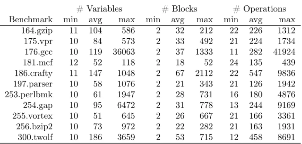
# Variables # Blocks # Operations
Benchmark min avg max min avg max min avg max
164.gzip 11 104 586 2 32 212 22 226 1312 175.vpr 10 84 573 2 33 492 21 224 1734 176.gcc 10 119 36063 2 37 1333 11 282 41924 181.mcf 12 52 118 2 18 52 24 135 439 186.crafty 11 147 1048 2 67 2112 22 547 9836 197.parser 10 58 1076 2 21 343 21 126 1942 253.perlbmk 10 61 1947 2 28 731 16 180 4876 254.gap 10 95 6472 2 31 778 13 244 9169 255.vortex 10 51 645 2 26 667 21 166 3361 256.bzip2 10 73 972 2 22 282 21 163 1931 300.twolf 10 186 3659 2 53 715 12 458 8691
Table 1: Program characteristics for optimized programs.
all liveness sets, i.e., for all basic blocks in the program, the live-in and live-out sets for all global variables. To obtain reproducible results, the execution time is measured using the instrumentation and profiling tool callgrind, which is part of the well-known valgrind tool. The measurements include the number of dynamic instructions executed as well as memory accesses via the instruction- and data caches. Using these measurements, a cycle estimate is computed for the liveness computation only, which minimizes the impact, on the measurements, of other compiler components and other programs running on the host machine.
The number of global variables, i.e., variables crossing basic block bound-aries, depends largely on the compiler optimizations performed before the live-ness calculation. Programs that are not optimized usually yield very few global variables since most values are kept in memory locations by default. However, optimized programs usually yield longer and more branched live-ranges. We thus investigate the behavior for optimized and unoptimized programs using the compiler flags -O2 and -O0 respectively. Table 1 shows the number of global variables, basic blocks, and operations for the optimized benchmark programs. The statistics for unoptimized programs are not shown, since the number of global variables never exceeds 19.
6.1
Pointer-Sets
The pointer-sets in LAO are implemented as arrays ordered by decreasing nu-meric identifiers. This results in rather fast set operations such as union and intersection at the expense of a rather expensive insertion. Due to the ordering of the pointer-sets, insertions are the fastest when the inserted variable is known to have an index number larger than all other variables in the set. The imple-mentation of the variable-by-variable algorithm thus performs best with the optimization for stack-like data structures presented in Section 5.2. Variables are considered in the right order to replace a logarithmic search by an insertion as first element. This is not the case for the use-by-use variant (Section 5.1). Note that the ordering of the set is preserved throughout the computation.
Figures 4 and 5 compare the average execution times measured for the in-dividual benchmarks in comparison to the our new non-iterative data-flow al-gorithm, for both unoptimized and optimized programs. The results indicate
164. gzip 175. vpr 176. gcc 181. mcf 186. craf ty 197. pars er 253. perlb mk 254. gap 255. vorte x 256. bzip2 300. twolf Aver age 0 0.2 0.4 0.6 0.8 1 1.2 1.4 1.6 1.8 1.521.64
forest use var
Figure 4: Speed-up with regard to our loop-forest-based approach using pointer-sets on unoptimized code.
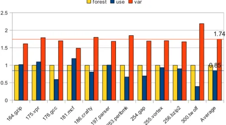
that the variable-by-variable algorithm outperforms the loop-forest-based ap-proach (Section 4) by 74% and 64% for optimized and unoptimized programs respectively. Indeed, the latter traverses all blocks for all variables and is bet-ter adapted for set operations, i.e., a bitset data structure. The results for the use-by-use algorithm highly depend on the characteristics of the input program. In particular for larger optimized programs such as gcc, perlbmk, and twolf the use-by-use approach shows poor results. This can be attributed to the unordered processing of the variables, resulting in costly insertion operations. Therefore, our tricks to design a stack-based implementation (Algorithm 7), at block level, of liveness analysis based on path-exploration, are worthwhile for ordered pointer-sets. The non-iterative data-flow analysis mainly applies set unification, which can be performed fast on the ordered set representation, and thus gains in comparison to the use-by-use variant.
164. gzip 175. vpr 176. gcc 181. mcf 186. craf ty 197. pars er 253. perlb mk 254. gap 255. vorte x 256. bzip2 300. twolf Aver age 0 0.5 1 1.5 2 2.5 0.85 1.74
forest use var
Figure 5: Speed-up with regard to our loop-forest-based approach using pointer-sets on optimized codes.
6.2
Bitsets
The use of bitsets in data-flow analysis is very common since most of the re-quired operations, such as insertion, union, and intersection, can be performed efficiently using this representation. In fact, our measurements show that these operations are so fast that the allocation and initialization of the bitsets becomes a major factor in the overall execution time of the considered algorithms.
Actually, cconsidering the program characteristics from Table 1, using sparse pointer-sets does not appear to be a good choice to represent liveness sets, and our experiments indicate that bitsets are overall superior. Indeed, the average number of variables per function is relatively low and does not exceed 184 for our benchmark set. In fact, 97% out of the 5848 functions contain less then 320 variables and almost 99% less then 640, which yields a size of merely 20 words on 32-bit machines in order to represent all variables as bitsets for almost all functions considered. It is thus not surprising that the baseline iterative data-flow algorithm using bitsets outperforms the same algorithm using pointer-sets by 69% and 85% for optimized and unoptimized input programs, and is thus even faster than the var-by-var approach on pointer-sets. The same is true for the three other algorithms studied in this paper.
For unoptimized programs, the results follow the observations for pointer-sets – see Figure 6. Since the number of variables is low and the extent of the respective live-ranges is short, the way sets are represented and how blocks are traversed is of less importance: the performances mainly reveal the intrinsic overhead of the different implementations (the constant hidden in the big O notation), including artifacts stemming from the host compiler and the host machine. The possible gain (for large sets) obtained by performing unions of bitsets instead of successive insertions does not compensate yet the overhead of the loop-forest-based algorithm. The program size, i.e., the number of basic blocks and operations, has less impact on the variable-by-variable algorithm, which simply iterates over the small set of global variables, with a very light precomputation of def-use chains. The two other approaches, however, have to traverse the CFG and its operations in order to find upward-exposed uses, possibly intermixed with function calls that are not inlined. Our loop-forest algorithm cannot reach the performances of the two path-exploration solutions, which show an average speed-up of 80% for the var-by-var algorithm and 63%
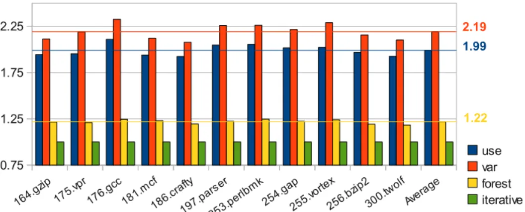
164.g zip 175.v pr 176.g cc 181.m cf 186.c rafty 197.p arser 253.p erlbm k 254.g ap 255.v ortex 256.b zip2 300.t wolf Avera ge 0.75 1.25 1.75 2.25 use var forest iterative 1.22 1.99 2.19
164.g zip 175.v pr 176.g cc 181.m cf 186.c rafty 197.p arser 253.p erlbm k 254.g ap 255.v ortex 256.b zip2 300.t wolf Avera ge 0.75 1.25 1.75 2.25 use var forest iterative 2.00 1.40 1.18
Figure 7: Speed-up w.r.t. iterative data-flow, bitsets, optimized programs. for the use-by-use variant. However, we already observe a clear improvement of 22%on average in comparison to the state-of-the-art iterative data-flow analysis. The characteristics of optimized programs are, however, different. The struc-ture of live-ranges is more complex and liveness sets are larger. For such pro-grams, the standard iterative data-flow analysis is still the worst but, now, the variable-by-variable algorithm is performing worse than the two others, see Figure 7. The loop-forest-based approach clearly outperforms both path-exploration algorithms, with speed-ups of 69% and 43% respectively. This is ex-plained by the relative cost of the fast bitset operations, in particular set unions, in comparison to the cost of traversing the CFG. Furthermore, the locality of memory accesses becomes a relevant performance factor. Both the use-by-use and the loop-forest algorithms operate locally on the bitsets surrounding a given program point. The inferior locality, combined with the necessary precomputa-tion of the def-use chains, explains the poor results of the variable-by-variable approach in this experimental setting.
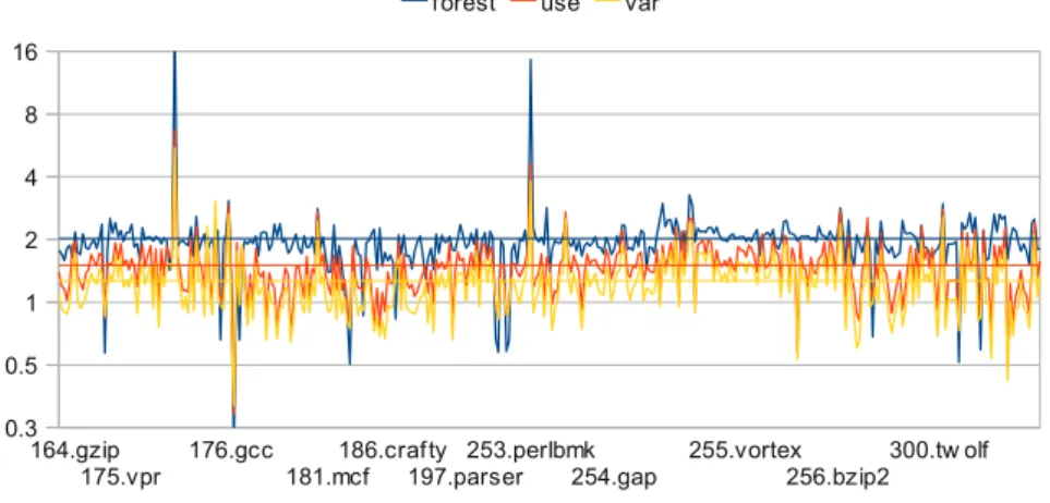
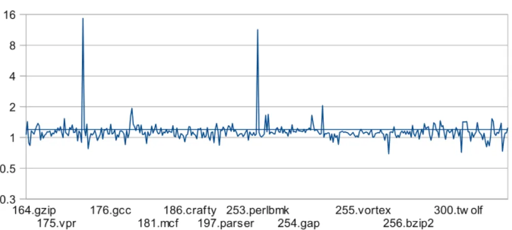
Figure 8 shows more detailed results, relative to the standard iterative data-flow approach, on a per-module basis, i.e., using one data point for every source file. The loop-forest and the use-by-use algorithm on average clearly outperform the iterative computation by a factor of 2 and 1.4 respectively. The extreme
164.gzip
175.vpr 176.gcc181.mcf186.crafty197.parser253.perlbmk254.gap 255.vortex256.bzip2300.tw olf 0.3 0.5 1 2 4 8 16
forest use var
cases showing speed-ups by a factor higher than 8 are caused by unusual – through relevant – loop structures in code generated by the parser generator bison(c-parse.c of gcc, and perly.c of perlbmk), which increase the number of iterations of the standard data-flow algorithm. On the other hand, all cases where the iterative approach outperforms the non-iterative are due to imple-mentation artifacts: the analyzed functions do not contain any global variables thus slight variations in the executed code, the code placement, and the state of the data-caches become relevant. The variable-by-variable approach is often even slower than the iterative one and on average shows a speed-up of 18%.
6.3
Non-SSA-Form Programs
In addition to the algorithms that require SSA form to be available, we also considered the path-based approach for programs not under SSA. The imple-mentation is based on pointer-sets, which showed the best speed-up for this particular algorithm variant in our previous experiments.
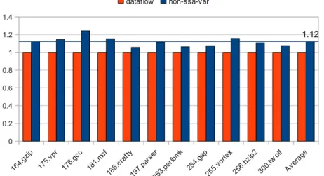
The algorithm requires a precomputation step in order to determine the sets of defined variables and upward-exposed uses. The relative speed-ups are thus diminished in comparison to the SSA-based algorithms, which have this infor-mation readily available. For unoptimized programs, the algorithm provides on average a gain of 12% in comparison to the standard iterative data-flow algo-rithm (also with pointer-sets), see Figure 9. The trend observed in our previous experiments is confirmed in this setting too. The results for optimized pro-grams are much better, with an average speed-up of 22% over all benchmarks (Figure 10). Also, the results per-module (Figure 11) follow the previous find-ings, albeit with reduced gains. An interesting detail is that the magnitude and the number of spikes indicating a slowdown in comparison to the data-flow algorithm is much smaller. Inspecting the involved benchmarks revealed that functions where the number of variables is exceedingly increased by SSA form and where the number of φ-operations is high are particularly affected.
If liveness sets are represented with bitsets, other alternatives may be de-signed, mixing the use-by-use approach with propagation of multiple variables together, as in standard data-flow algorithms. However, such a study is out of the scope of this paper, which is primarily devoted to SSA programs.
164. gzip 175. vpr 176. gcc 181. mcf 186. craf ty 197. pars er 253. perlb mk 254. gap 255. vorte x 256. bzip2 300. twolf Aver age 0 0.2 0.4 0.6 0.8 1 1.2 1.4 1.12 dataflow non-ssa-var
Figure 9: Speed-up of the variable-by-variable approach relative to iterative data-flow analysis using pointer-sets on unoptimized non-SSA programs.