A Queueing System for Modeling a File Sharing Principle
Florian Simatos and Philippe Robert
INRIA, RAP project
Domaine de Voluceau, Rocquencourt 78153 Le Chesnay, France
{Florian.Simatos,Philippe.Robert}@inria.fr
Fabrice Guillemin
Orange Labs 2, Avenue Pierre Marzin
22300 Lannion
[email protected]
ABSTRACT
We investigate in this paper the performance of a simple file sharing principle. For this purpose, we consider a sys-tem composed of N peers becoming active at exponential random times; the system is initiated with only one server offering the desired file and the other peers after becoming active try to download it. Once the file has been downloaded by a peer, this one immediately becomes a server. To inves-tigate the transient behavior of this file sharing system, we study the instant when the system shifts from a congested state where all servers available are saturated by incoming demands to a state where a growing number of servers are idle. In spite of its apparent simplicity, this queueing model (with a random number of servers) turns out to be quite dif-ficult to analyze. A formulation in terms of an urn and ball model is proposed and corresponding scaling results are de-rived. These asymptotic results are then compared against simulations.
Categories and Subject Descriptors
C.4 [Computer Systems Organization]: Performance of Systems—modeling techniques, performance attributes
General Terms
Algorithms, Performance
1. INTRODUCTION
This paper analyzes the performance of a simple file shar-ing principle durshar-ing a flash crowd scenario when a popular content becomes available on a peer-to-peer network. It is supposed that a given peer is willing to share a given file with a community of N peers, which are initially asleep. An asleep peer becomes active at some random time, i.e., it tries to download the file from a peer having the complete file. Once a peer has downloaded the file, it immediately becomes a server from which another peer can download the file. To simplify the model, we assume that the file is in one piece
Permission to make digital or hard copies of all or part of this work for personal or classroom use is granted without fee provided that copies are not made or distributed for profit or commercial advantage and that copies bear this notice and the full citation on the first page. To copy otherwise, to republish, to post on servers or to redistribute to lists, requires prior specific permission and/or a fee.
SIGMETRICS’08, June 2–6, 2008, Annapolis, Maryland, USA.
Copyright 2008 ACM 978-1-60558-005-0/08/06 ...$5.00.
and not segmented into chunks; the time needed to down-load the file from one server is supposed to be random in order to take into account the diversity of upload capacities of peers.
The goal of this paper is to understand how the network builds up in this situation as peers join the system. In partic-ular, we are interested in analyzing the growth of the num-ber of available servers in the system. Note that there are eventually as many servers as peers since each of them can complete the file download.
In spite of its apparent simplicity, the analysis of the sys-tem is quite difficult because we have to cope with a network comprising a random number of servers: When peers com-plete their download, they become new servers so that the number of servers is continually increasing. It is assumed that an incoming peer chooses a server with the smallest number of queued peers. Other routing policies are consid-ered at the end of this paper.
The analysis performed in this paper substantially differs from earlier studies appeared so far in the technical litera-ture in the sense that we consider the transient formation of a network of peers. Yang and de Veciana [17] considered a similar setting which they analyzed with results related to branching processes to describe the exponential growth of the number of servers. Our goal in this paper is precisely to obtain more detailed asymptotics of this transient regime. Except the paper by Yang and de Veciana [17], most of the papers published so far on the performance of peer-to-peer systems assume that peers join and leave the system and that a steady state regime exists. The problem is then to evaluate the impact of some parameters of the file sharing protocol on the equilibrium of the system. Different tech-niques can be used to perform such an analysis, for instance by using a Markovian chain to describe the state of the sys-tem, possibly by using approximation techniques when the state space related to the number of peers in the system is too large. See Ge et al. [7]. A fluid flow analysis with an underlying Markovian structure is proposed in Cl´evenot and Nain [5] in order to model the Squirrel peer-to-peer caching system. In Qiu and Srikant [14], the authors directly use a fluid approximation to study the steady state of a peer to peer network, subsequently complemented by diffusion vari-ations around the steady state solutions. In Massouli´e and Vojnovi´c [13], the authors study the performance of a file sharing system via a stochastic coupon replication formula-tion, a coupon corresponding to a chunk of a file. The goal of this study is to understand the impact of the policy ap-plied by users for choosing coupons on the performance of
the system. The system is studied in equilibrium as in Qiu and Srikant [14].
The rest of this paper is organized as follows: In Section 2, we describe the system under consideration and some heuris-tics to study the system are presented. It turns out that the dynamics of the system can be decomposed in two regimes. In the first one, there are almost no empty servers and we establish an analogy with a random urn and ball problem on the real line. By approximating the probability of se-lecting an urn by its mean value, we analyze in Section 3 the corresponding deterministic urn and ball problem. The analysis for the random urn and ball problem is much more complicated to analyze. The complete analysis is done in [12] and only the main results are summarized in Section 5. In Section 6, we support via simulation the different approx-imations and heuristics made in this paper to analyze the file sharing system. Concluding remarks are presented in Section 7.
2. MODEL DESCRIPTION
2.1 Problem formulation
We consider throughout this paper a system composed of N peers interested in downloading a given file. At the be-ginning, only one peer (the initial server) has the file and other peers are asleep. When becoming active, after an ex-ponentially distributed duration of time with parameter ρ, a peer tries to download the file from the server that is the less loaded in terms of number of queued peers. In partic-ular, the first peer becoming active downloads the file from the initial server. The time needed to download the file is assumed to be exponentially distributed with mean 1.
Exponential distributions.
The hypothesis on the distribution on the duration of the time for a peer to be active is quite reasonable: this is a classical situation when a large number of independent users may access some network. The assumption on the duration of the time to download is not realistic in practice since this quantity is related to the size of the file requested whose distribution is more likely to be bounded by the maximal size of a chunk. As it will be seen, even within this simplified setting (in order to have a nice probabilistic description of the process), mathematical problems turn out to be quite intricate to solve. In this respect, our study could be seen as a first step in the analysis of flash crowd scenarios. It turns out that our current investigations in the general case seem to show that the exponential distribution does not have a critical impact on the qualitative behavior as long as the FIFO policy is used by servers. Mathematically, however, numerous technical points are not settled in this case.
We assume that peers requesting the file from the same server are served according to the FIFO discipline. Note that, because of the exponential distribution assumption, this case is equivalent to the Processor-Sharing discipline, i.e., when N peers are present for a duration of time h, each of them receives the amount of work h/N . Just af-ter completing the file download, a peer immediately be-comes a server from which other peers can retrieve the file. The problem of “free riders”, i.e., peers who do not become servers after service completion, is not discussed here. As it will be seen, this feature does not change significantly the qualitative properties of the system. The problem of servers
who disconnect while they have downloads in progress will not be discussed in this paper.
It is worth noting that the model under consideration de-scribes a “flash crowd” scenario. Indeed, a peer having a file accepts to share it with other peers and we are interested in the dynamics of the sharing process when a large population of peers tries to download the file. Moreover, since the du-rations for which these peers stay inactive are independent and identically distributed, the flow of arrivals of peers into the system is not stationary, but rather accumulates at the beginning and is then less and less intense. We are hence interested in the transient regime of the system. Contrary to the earlier studies [7, 13, 14], we are not interested in the steady state regime of the system, where peers continually join and leave the system.
It is intuitively clear that there should exist two different regimes for this system. Initially, it starts congested: many peers request the file, and only a few servers are available. Afterward, the situation is reversed: there are a large num-ber of servers and only a few requests from the remaining inactive peers.
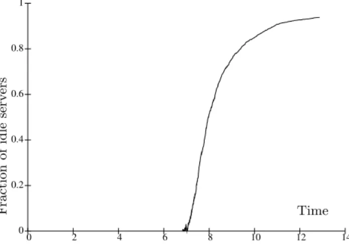
These two regimes clearly appear in Figure 1 depicting the simulation results with N = 106 peers and ρ = 5/6. It shows that before time T ≈ 7 time units (or equivalently mean download times), there are almost no empty servers, while after that time, more and more servers are empty until all peers have completed their download. But as long as the input rate is high, a new server immediately receives a customer. This is all the more true under the routing policy considered, since new peers entering the system choose an empty server if any.
0 0.2 0.4 0.6 0.8 1 0 2 4 6 8 10 12 14 F ra ct io n o f id le se rv er s Time
Figure 1: Fraction of idle servers: N =106 and ρ=5/6.
2.2 A Non-Trivial Queueing Model
From the above description, the system can be represented by means of a queueing system with a random number of queues. Initially, the system is composed of a single server, and once a customer has completed its service, it becomes a new server. Since only a finite total number of customers is considered, there are eventually as many servers as cus-tomers.
When peer inter-arrival times and file download times are assumed to be exponentially distributed, a minimal Marko-vian representation of this queueing model requires the
knowl-edge of the number of peers which are still asleep and the number of peers connected to each server. Since this Markov process is ultimately absorbing (all peers are servers at the end), the transient behavior of the system is of course the main object of interest in the analysis. Even in very sim-ple queueing systems, the transient behavior is delicate to analyze and much more difficult to describe than the station-ary behavior. The classical M/M/1 queue is a good (and simple) example of such a situation when transient char-acteristics are not easy to express with simple closed form formulas. See Asmussen [1] for example.
Given the multi-dimensional description (with unbounded dimension) of the Markov process, the system considered here is much more intricate and challenging. To analyze this system, a simpler mathematical model with urns and balls is used to investigate the duration of the first regime of this system. The specific point addressed in this paper is to describe the transient behavior when N becomes large.
2.3 Modeling the First Regime
Initially, the input rate is large and therefore a newly cre-ated server receives very quickly many requests from the nu-merous peers becoming active. The first regime described in the previous section and illustrated in Figure 1 is hence char-acterized by the fact that the duration times during which some servers are idle are negligible. In a second phase the number of empty servers begins to be significant before in-creasing very rapidly in the last phase. This phenomenon is discussed in Section 6. For the first regime, this leads us to describe the dynamics of the system as follows.
Let Sn be the time at which the n-th server is created,
with the convention that S0 = 0 (the initial server has
la-bel 0). During the n-th time interval (Sn−1, Sn) for n ≥ 1,
there are by definition exactly n servers. So if we assume, as argued above, that empty servers are negligible during the first regime, Sn− Sn−1 is well approximated by the
mini-mum of n independent exponential random variables with parameter 1. The random variable Sn can thus be
repre-sented as Sn−1+ En1/n, where E1nis an exponential random
variable with parameter 1 independent of the past. In par-ticular, during the first regime, the following approximation is accurate.
Approximation 1. For n ∈ N, as long as the system is still in the first regime, the instant of creation of the n-th server is given by Sn≈ Tn, where
Tn= n X k=1 E1 k k , (1) and E1
n being i.i.d. exponential random variables with unit
mean.
Despite this approximation seems to be quite rough, (a rigorous mathematical formulation of the approximation Sn≈
Tnseems to be difficult to establish), Proposition 1 and the
subsequent discussion below provide strong arguments to support its accuracy. In the definition of the above approx-imation, it is essential to determine the duration of the first regime, in particular to know whether Sn≈ Tnholds or not.
For instance, one could consider as definition for the du-ration of the first regime the last time when there are no empty servers. This time is unfortunately not a stopping time and turns out to be much more difficult to study. In
Section 6, we shall consider different heuristics for evaluat-ing the length of the first regime. We start the analysis by introducing the index ν defined as follows.
Definition 1. The duration of the first regime is defined as Sν, where ν is the first index n ≥ 1 so that one or no
peer arrive between Sn−1and Sn.
According to this definition, the first regime lasts as long as between the creation of two successive servers, at least two peers arrive in the system. The intuition behind this heuris-tic is that, because of the policy for the choice of servers, if many peers arrive in any interval, then the least loaded servers will receive requests from arriving peers. Thus, as long as many peers arrive, it is quite rare for a server to remain empty.
The phase transition should occur when the number of arrivals between the creation of two successive servers is not sufficient to give work to empty servers which are created. In particular, if no peers arrive in some interval, then there will be at least two empty servers at the beginning of the next time interval. So the first time when only a few peers arrive in some interval should be a good indication on the current state of the system. A probably more natural heuris-tic would have been to consider the first interval in which no peer arrives. Nevertheless, an argument in favor of the former heuristic is that it enjoys the following nice property. Proposition 1. For n < ν, at most two servers are si-multaneously empty in the n-th interval (Sn−1, Sn).
Proof. The proof is by induction. For n = 1, the prop-erty is trivial, since there is only one server in the first in-terval. Consider now 1 < n < ν, and suppose that the property holds for n − 1. Since at least two peers arrive in the (n − 1)-th interval, and since these peers are necessar-ily routed to empty servers, if any, there is no empty server just before Sn−1. Therefore, just after Sn−1, there are at
most two empty servers, and so the property holds as long as n < ν.
We are now able to justify Approximation 1. Indeed, for n < ν, the number of non idle servers is between n − 2 and n. For n large, approximately n servers are busy, thus Sn−
Sn−1is close in distribution to an exponentially distributed
random variable with parameter n. During the first time intervals, the number of empty servers is negligible. Indeed, consider any finite index n, then it is easy to see that the mean number of peers that arrive in the n-th interval is proportional to N . So after the creation of the n-th server, the mean time before the next arrival behaves as 1/N , and so is very small when N is large. This intuitively shows that the fraction of idle servers is initially negligible, which justifies Approximation 1.
From now on, the identification of Sn and Tn, where the
sequence (Tn) is defined by Equation (1), is assumed to hold.
Results on Tncan be assumed to hold for Snwhen n < ν.
3. URN AND BALL PROBLEM
Denote by (Eiρ, 1 ≤ i ≤ N ) an i.i.d. sequence of exponen-tially distributed random variables with parameter ρ. For i ≤ N , Eρ
i is the time at which the i-th peer becomes active.
We introduce the following urn and ball model on the real line: The interval (Tn−1, Tn) is the n-th urn and the
variables (Eρ
i, 1 ≤ i ≤ N ) are the locations of N balls thrown
on the real line. The set {Tn−1 ≤ Eiρ≤ Tn} is simply the
event that the i-th ball falls into the n-th urn. Conditionally on the sizes of the urns, i.e., on T = (Tn), we have that the
probability of such an event (which does not depend on i) is Pn= P (Tn−1< Eiρ< Tn| T )
= e−ρTn−1“1 − e−ρE1n/n
”
, (2)
where the random variables E1
n, n ≥ 1, are independent and
exponentially distributed with mean unity.
With the above formulation, we have then to deal with the following urn and ball model:
1. A random probability distribution P = (Pn) is given
(urns with random sizes).
2. N balls are thrown independently according to the probability distribution P.
It is worth noting that the above urn and ball model has an infinite number of urns. In addition, although urn and ball problems have been widely studied in the literature, our model presents a remarkable feature: For i ≥ 1, a ball falls into urn i with probability Pi which is a random variable,
but conditionally on the sequence (Pn), this is a classical
urn and ball problem. Mathematical results for urn models with random distributions are quite rare. See Kingman [11] and Gnedin et al. [8] and the references therein where some related models have been investigated.
The random model under consideration will give us some information on the behavior of our system. The following proposition establishes a simple but important characteriza-tion for the asymptotic behavior of (Pn).
Proposition 2. Let (E1i), i ≥ 1, be independent
expo-nential random variables with parameter 1. Then, for n ∈ N Tn= n X k=1 E1k k dist. = max 1≤k≤nE 1 k, (3)
and the sequence (Tn− log n) converges almost surely to
a finite random variable T∞ whose distribution is given by
P(T∞≤ x) = exp(− exp(−x)) for x ∈ R.
The conditional probability Pn of throwing a ball into the
n-th urn can be written as
Pn= ρ nρ+1Xn−1Zn, (4) where Zn= n ρ “ 1 − e−ρEn1/n ” and Xn−1= nρe−ρTn−1
are independent random variables. As n goes to infinity, Xn
(resp. Zn) converges in distribution to X∞ (resp. Z∞). The
convergence of (Xn) to X∞ holds almost surely and in Lq,
for any q ≥ 1.
The limiting variable Z∞ has an exponential distribution
with parameter 1 and X∞ has a Weibull distribution with
parameter 1/ρ,
P(X∞≥ x) = e−x1/ρ, x ≥ 0. (5)
Proof. Let E(1) ≤ E(2) ≤ · · · ≤ E(n) be the variables
(E1
k, 1 ≤ k ≤ n) in increasing order. In particular E(n) =
max1≤k≤nEk1. With the convention E(0)=0, due to
stan-dard properties of the exponential distribution, the variables E(i+1)−E(i), i = 0,. . . , n−1 are independent and the
vari-able E(i+1)− E(i)is the minimum of n − i exponential
vari-ables with parameter 1, i.e., has the same distribution as E1
n−i/(n−i). The distribution identity (3) then follows.
Since Zndist.= n/ρ(1 − exp(−ρE1/n)), it converges in
dis-tribution to an exponential disdis-tribution with parameter one. Define Mn= n X k=1 E1 k− 1 k = Tn− Hn,
where (Hn) is the sequence of harmonic numbers, Hn =
1+1/2+· · ·+1/n. The sequence (Mn) is clearly a martingale,
it is bounded in L2 since EMn2= n X k=1 E`E1 k− 1 ´2 k2 = ∞ X k=1 1 k2 < +∞.
It therefore converges almost surely. See Williams [16] for example. The almost sure convergence of (Tn− log n) =
(Mn+ Hn− log n) is thus proved. Identity (3) gives that,
for x ≥ 0,
P(Tn− log n ≤ x) = (1 − e−x−log n)n∼ e−e−x, as n goes to infinity.
Since
Xn= e−ρMneρ(log(n+1)−Hn),
one gets the almost sure convergence of (Xn). It is easy to
check that, for q ≥ 0, E(Xnq) = (n + 1)qρ n Y i=1 1 1 + qρ/i = (n + 1)qρ Γ(n) Γ(n + qρ)Γ(qρ) ∼ Γ(qρ), (6) when n → ∞, where Γ is the usual Gamma function, and where the last equivalence easily comes from Stirling’s For-mula. In particular, for any q ≥ 0, the q-th moment of Xn is therefore bounded with respect to n. One deduces
the convergence in Lq of the sequence (Xn). Since Xn =
exp(−ρ(Tn− log(n + 1))), one has the equality in
distribu-tion X∞= exp(−T∞) which gives the law of X∞.
It is important to note that the probability distribution P = (Pn) is a random element in the set of probability
distributions on N. The decay of this distribution follows a power law with parameter ρ + 1, because according to the previous proposition, nρ+1Pn converges in distribution
to ρX∞Z∞. Using the asymptotic behavior derived in (6)
with q = 1, it is easy to see that the average probability for a ball to fall into the n-th urn satisfies the following relation
E(Pn) ∼ρΓ(ρ)
nρ+1. (7)
This equivalence suggests the introduction of a deterministic version of the urn and ball problem considered.
4. DETERMINISTIC PROBLEM
4.1 Description
Denote by Q = (qn) a probability distribution on N such
that
lim
n→+∞n δq
n= α, (8)
for some α > 0 and δ > 1. For each n, qn can be seen
as the probability for a ball to fall in the n-th urn. When δ = ρ + 1 and α = ρΓ(ρ), the sequence (qn) has the same
asymptotic behavior as E(Pn) given by Equation (7). Hence,
this model may be considered as the deterministic equivalent of the urn and ball problem defined in the previous section. For the sake of clarity, the problem with the probability distribution P (resp. Q) will be referred to as the random (resp. deterministic) problem.
The deterministic problem amounts to throwing N ex-ponential variables with parameter ρ on the half-real line, where this line has been divided into deterministic intervals (tn−1, tn) with tn= ETn. The main quantity of interest in
the following is the asymptotic behavior with respect to N of the index of the first urn that does not receive any ball.
Definition 2. Let us denote by ηiR(N ) (resp. ηiD(N )) the
number of balls in the i-th urn when N balls have been thrown in the random (resp. deterministic) urn and ball problem, and define
νR(N ) = inf{i ≥ 1 : ηRi (N ) = 0}, (9)
νD(N ) = inf{i ≥ 1 : ηDi (N ) = 0}.
In view of Definition 1, to investigate the duration of the first regime of the system, the asymptotic behavior of the sequences (νR(N )) and (νD(N )) is analyzed. Since we con-sider that the first regime lasts until one or no peers arrive between the creation of two successive servers, we should have to consider ν′(N ) = inf{i ≥ 1 : ηi(N ) ≤ 1} to be
rigorous. In fact, the mathematical analysis of the index of the first empty urn can easily be extended to the first urn that receives less than k balls. For the sake of simplicity, we therefore only treat the case k = 0. Neither the orders of magnitude nor the asymptotic behaviors established in the following are affected by the value of k, and in particular if we consider 1 instead of 0.
To conclude this section, let us give a rough approximation of the correct order of magnitude for νR(N ) and νD(N ) as N
gets large. Rigorous mathematical analysis is carried out in Section 4.2, while Section 6 compares the insights provided by the two models.
For i ≥ 1, E(ηiD(N )) = N qi∼ αN/iρ+1. Hence, in the
de-terministic model, a finite number of balls will fall in the i-th urn as soon as i is of the order of N1/(ρ+1) as N becomes
large. Hence we expect that in the deterministic model, νD(N )/k(N ) converges in distribution for k(N ) = N1/(ρ+1). Theorem 1 below shows that the location of the first empty urn is in fact slightly smaller than N1/(ρ+1), i.e., of the
or-der of (N/ ln N )1/(ρ+1). Nevertheless this heuristic approach gives the correct exponent in N .
Although E(ηR
i (N )) has the same asymptotic behavior,
the corresponding heuristic approach in the case of the ran-dom model is more subtle. Indeed, we have
E(ηiR(N )) = N E(Pi) ∼ N ρΓ(ρ)/iρ+1,
so the number of balls falling in the i-th urn should be of the order N i−ρ−1. However, in the random model, the
i-th interval is wii-th random lengi-th E1
i/i. So from Ti−1, the
next point Ti is at a distance Ei1/i and the first ball is at
a distance corresponding to the minimum of N i−ρ−1 i.i.d.
exponential random variables with parameter 1. Thus, with this approximation, the i-th interval is empty with proba-bility P „ E1 i i ≤ iρ+1 N E 1 0 « = 1 1 + N/iρ+2.
When N → ∞, this probability is non negligible as soon as i is of order N1/(ρ+2), which is significantly below what
we found in the deterministic case. Theorem 2 below shows that this is indeed the correct answer. The order of mag-nitude is one order smaller, compared to the deterministic case, because of the variability of the intervals size: to some extent, a very small interval is generated, so that no balls fall in it, while in the deterministic case, some balls would have.
4.2 Asymptotic Analysis
Cs´aki and F¨oldes [6] gives the asymptotic behavior of the distribution of νD when N is large. A more complete de-scription of the locations of the first empty urns (and not only for the first one) can however be achieved. For this purpose, the variable WNk is defined as the number of empty
urns whose index is less than k when N balls have been thrown. This random variable is formally defined as
WNk = k
X
i=1
IN,i, with IN,i=1
{ηD
i (N)=0}. (10)
The distribution of Wk
N is analyzed when k is dependent
on N . First, some estimates for the mean value and the variance of WNk are required.
Proposition 3. Assume that the sequence (qi) is
non-increasing. For x > 0, if κx(N ) = $„ αδ N log N «1/δ» 1 +1 + δ δ log log N log N + log x log N –% , (11) where⌊y⌋ is the integral part of y > 0, then
lim N→+∞ E“Wκx(N) N ” = (αδ)1/δx. (12) Proof. For k, N ∈ N E “ WNk ” = k X i=1 (1 − qi)N. (13) For 0 ≤ x ≤ 1, 0 ≤ e−Nx− (1 − x)N≤ xN(1 − xN)N−1,
where xNis the unique solution to the equation exp(−N x) =
(1 − x)N−1, since the function x → e−Nx− (1 − x)N has a
maximum at point xN. It is easily seen that N xN ≤ 2 (in
fact N xN→ 2 as N → +∞), so that for N ≥ 1
sup
0≤x≤1
˛ ˛
With this relation, we obtain ˛ ˛ ˛ ˛ ˛E “ WNk ” − k X i=1 e−Nqi ˛ ˛ ˛ ˛ ˛≤ 2k N,
so that for k = κx(N ) and large N , (1−qi)Ncan be replaced
with exp(−N qi) in the expression of E(WNk).
For the sake of simplicity, we assume that qi = α/iδ, for
i ≥ 1. The general case of a non-increasing sequence (qi)
follows along the same lines since the crucial relation below holds true with a convenient function q. One defines q(x) = α min(x−δ, 1) for x ≥ 0. Z k 0 e−Nq(u)du ≤ k X i=1 e−Nqi ≤ Z k+1 1 e−Nq(u)du.
The difference between these two integrals is bounded by 2 exp(−αN/kδ). Now take k = k(N ) with k(N ) with the same order of magnitude as (N/ log N )1/δ, say, k(N ) ∼
A(N/ log N )1/δ for some A > 0. We have
E “ WNk(N)”= Z k(N) 1 e−Nq(u)du + o(1). The right hand side of the above equation is given by
Z k(N) 1 e−αNu−δdu =(αN ) 1/δ δ Z αN αNk(N)−δ e−uu−(δ+1)/δdu. (15)
Now let H(N ) = αN k(N )−δ and consider eH(N)H(N )(1+δ)/δ Z αN H(N) e−uu−(δ+1)/δdu = Z αN H(N) e−(u−H(N)) „H(N ) u «−(δ+1)/δ du = Z αN/H(N) 1 H(N )e−H(N)(u−1) 1 u(δ+1)/δdu ∼ Z +∞ 0 H(N )e−H(N)u 1 (1 + u)(δ+1)/δdu ∼ 1, since N/H(N ) → +∞ and H(N ) → +∞ as N → +∞. Therefore, an equivalent expression of the integral in the right hand side of Equation (15) has been obtained. Gath-ering these results, we obtain
E “ WNk(N)”= (αN ) 1/δ δ e −H(N) H(N )−(1+δ)/δ+ o(1) ∼ 1 αδ k(N )1+δ N exp “ −αNk(N)−δ”. (16) Relation (12) is obtained by taking k(N ) = κx(N ).
The following proposition shows the equivalence of the variance and the mean value of Wκx(N)
N under a convenient
scaling. This result is crucial to prove the limit theorems of this section.
Proposition 4. Assume that the sequence (qi) is
non-increasing. For x > 0, let κx be defined by Equation (11),
then lim N→+∞ Var “ Wκx(N) N ”. E “ Wκx(N) N ” = 1. (17)
Proof. For k ≥ 1, by using Equation (13) (which does not depend on α). (E[WNk])2= X 1≤i,j≤k (1 − qi− qj+ qiqj)N, and E[(WNk)2] = E[WNk] + X 1≤i6=j≤k (1 − qi− qj)N,
so that, to prove the equivalence of Var(Wk
N) and E(WNk),
it is sufficient to show that the quantities X 1≤i,j≤k h (1 − qi− qj+ qiqj)N− (1 − qi− qj)N i and k X i=1 (1 − 2qi)N
are negligible with respect to E(Wk
N). Since we consider
k(N ) = κx(N ), this amounts to show that these quantities
are o(1) by Proposition 4. The second term is the expected number of empty urns for the distribution (˜qi) such that
˜
qi∼ 2α/iδ. Estimate (16) shows that κXx(N) i=1 (1 − 2qi)N∼ 1 2αδ κx(N )1+δ N exp “ −2αNκx(N )−δ ” = o“EWκx(N) N ” .
By using the fact that for a ≥ b ≥ 0, aN− bN ≤ N(a −
b)aN−1, the second term satisfies
X 1≤i,j≤k h (1 − qi− qj+ qiqj)N− (1 − qi− qj)N i ≤ N X 1≤i,j≤k qiqj(1 − qi− qj+ qiqj)N−1 = 1 N k X i=1 N qi(1 − qi)N−1 !2 . (18) By using a similar method as in the proof of Proposition 3, we obtain the equivalence
k(N)X i=1 N qi(1 − qi)N−1∼ Z k(N) 1 N q(u)e−Nq(u)du ∼ (αδ)1/δαx N κx(N )δ = (αδ)1/δx log N.
This equivalence together with Equation (18) complete the proof of the proposition.
Theorem 1. Let (qn) be a non-increasing sequence
sat-isfying Relation (8). For x > 0 and N ∈ N, set κx(N ) = $„ αδ N log N «1/δ„ 1 +1 + δ δ log log N log N + log x log N «% . When N goes to infinity, the variable Wκx(N)
N converges in
distribution to a Poisson random variable with parameter (αδ)1/δx.
The index νD(N ) of the first empty urn defined by
Equa-tion (9) is such that the variable (log N )(1+δ)/δ
(αδN )1/δ ν
D(N ) − log N −1 + δ
δ log log N (19)
converges in distribution to a random variable Y defined by P(Y ≥ x) = exp
“
−(αδ)1/δex”, x ∈ R.
Proof. Chen-Stein’s method is the basic tool in the proof of the theorem. See Barbour et al. [4] for a detailed presen-tation of this powerful method. Let N , and k be in N and 1 ≤ i0 ≤ k. The variable WNk conditioned on the event
{IN,i0 = 1} has the same distribution as the number of
empty urns when the balls in the i0-th urn are thrown again
until the i0-th urn is empty. It follows that the number of
balls in any other urn is larger than in the case when they are assigned at first draw. One deduces that for i 6= i0,
P(IN,i= 1 | IN,i
0 = 1) ≤ P (IN,i= 1) .
The variables (IN,i, 1 ≤ i ≤ k) are therefore negatively
cor-related, see Barbour et al. [4]. Then, by [4, Corollary 2.C.2], the following relation holds,
X p≥0 ˛ ˛ ˛ ˛ ˛P(W k n= p) − E`Wk N ´p p! e −E(Wk N) ˛ ˛ ˛ ˛ ˛ ≤ 1 − Var“WNk ”. E“WNk”. By taking k = κx(N ) and by using Propositions 3 and 4, we
obtain the convergence in distribution of Wκx(N)
N to a
Pois-son distribution with parameter (αδ)1/δx. The last part of
the theorem is a simple consequence of the identity P(WNk =
0) = P(νD(N ) > k).
The convergence in distribution of νD(N ) has been proved
by Cs´aki and F¨oldes [6] with a different method. Our result gives a more accurate description of the location of empty urns (and not only the first one) near the index κx(N ).
The following corollary is a straightforward application of the detailed asymptotics obtained in the above theorem.
Corollary 1 (Cutoff phenomenon). Under the
as-sumption of Theorem 1, if
k(N ) = (N/log N )1/δ,
then, as N goes to infinity, the following convergence in dis-tribution holds: For β > 0,
WNβk(N)−→ (
+∞ if β > (αδ)1/δ,
0 if β < (αδ)1/δ.
So far, only indexes of empty urns have been considered. The result below shows that the first empty urn happens at a time of the order of log N . Remembering the approximation of the peer to peer system, it suggests that the time the system begins to serve quickly the incoming peers should be of the same order.
Corollary 2 (First Empty Urn). Let
TD(N ) = TνD(N)=
νDX(N) k=1
Ek1
k . (20)
Under the assumptions of Theorem 1, the quantity δTD(N ) − log N + log log N − log(αδ)
converges in distribution to T∞, where T∞ is the random
variable defined in Proposition 2.
Proof. If VN is the variable defined by Expression (19),
then
δ log νD(N ) − log(N ) + log log N − log(αδ) = δ log „ 1 log N „ VN+ log N + 1 + δ δ log log N «« . Since by Theorem 1 the sequence (Vn) converges in
distri-bution, it implies that the right hand side of the above ex-pression converges in distribution to 0. Proposition 2 shows that E11+ E21 2 + · · · + E1n n − log n converges almost surely to T∞.
5. RANDOM PROBLEM
For the random model, the probability Pnof selecting the
n-th urn is given by Equation (4) of Proposition 2. In the (almost sure) limit as n goes to infinity, Xn ∼ X∞ and
in distribution, Zn is asymptotically an exponentially
dis-tributed random variable with parameter 1. The sequence (Pn) can be approximated by “ ρ nρ+1X∞E 1 n ” ,
where (En1) are i.i.d. exponential variables with unit means.
In spite of the fact that the decay of Pn follows a power
law, the random factor plays an important role. This factor is composed of two variables, one (namely X∞) is fixed once
for all and the other (namely Zn) changes for every urn.
The fact that Zn, related to the “width” of the n-th urn, can
be arbitrarily small with a positive probability suggests that the index νR of the first empty urn should be smaller than
the corresponding quantity for the deterministic case. This is indeed true but the situation in this case is much more complex to analyze. The complete analysis of the random case is given in [12], and only sketches of proof are given for Proposition 5 and Theorem 2 in the present paper. It must be noticed that a similar problem where X∞and the
sequence (E1
n, n ≥ 1) are independent is fairly easy to solve.
However here, these random variables are dependent, and this dependency requires quite technical probabilistic tools. To derive asymptotic results for νR, as in the previous
section, the asymptotic behavior of the random variable Wk N defined by Wk N= k X i=1
IN,i with IN,i=1
{ηR i(N)=0}.
is investigated. Although in the deterministic case, Chen-Stein’s method makes it possible to reduce the analysis of Wk
Nto its first and second moments, this is no longer the case
for the random problem. Indeed, because of the variability of the urns sizes, the random variables (IN,i, 1 ≤ i ≤ k) are
no longer negatively correlated. Moreover, the ratio of the expected value to the variance of WNk(N) does not converge
to 1 for a convenient sequence (k(N )) as in the determin-istic case (Proposition 4), which suggests that if a limit in distribution exists, it cannot be Poisson.
As was pointed out in Hwang and Janson [10], the se-quence (N Pi, 1 ≤ i ≤ k) plays a central role in the limiting
behavior of (Wk
N). The following technical proposition gives
a result on the asymptotic behavior of this sequence. It is important since it introduces the scale N1/(ρ+2)which turns
out to be the correct scaling for the variable νR(N ); see [12]
for the proof.
Proposition 5. Let x > 0. When N goes to infinity, the random sequence (N Pi, 1 ≤ i ≤ xN1/(ρ+2)) converges
in distribution to a doubly stochastic Poisson process with a random intensity xρ+2`X
∞ρ(ρ + 2)´−1.
Proof. Because of the technicality involved, we only give a sketch of the proof. The reader is referred to [12] for more details.
To prove the convergence of the sequence of point pro-cesses NN = Pk(N)i=1 δ{NPi} with k(N ) = xN
1/(ρ+2), it is
enough to show the convergence of the Laplace transforms of these point processes applied to some suitable functions. Non-negative continuous functions with a compact support would be enough to prove the result, but the next theorem requires a slightly stronger result, namely it requires the converge of Laplace transforms for non-negative continuous functions vanishing at infinity, i.e., that for any function f ≥ 0 continuous vanishing at infinity, we have
lim
N→+∞
E“e−NN(f )”= E“e−N∞(f )”
where, conditionally on X∞, N∞is a Poisson process with
intensity xρ+2X−1
∞/(ρ + 2).
The general idea is to condition on the random variable X∞. However, for each n ≥ 1, X∞ and Zn are dependent,
so that this cannot be directly done. Instead, the first step of the proof is to show that only the last terms of the point process matter, i.e., that E(e−NN(f )) and E(e−
Pk(N ) β(N )f (NPi))
have the same limit, for any sequence β(N ) ≪ k(N ). So we are left with large indexes i ≥ β(N ), for which the approxi-mation Pi= ρi−ρ−1XiZi≈ ρi−ρ−1Xβ(N)Zican be justified.
The main tool behind this approximation is Doob’s Inequal-ity applied to the reversed martingale
Mn=
X
k≥n
(Ek− 1)/k.
And now, due to this approximation, it is perfectly rig-orous to condition on FN = σ(Ek, k < β(N )): since for
i ≥ β(N ), Zi is independent of Xβ(N), we are exactly left
with proving the result for the sequence of point processes N′
N =
Pk(N)
β(N)δ{NxNi−ρ−1Zi}with any converging sequence
xN→ x∞(xNhas to be thought as being equal to ρXβ(N)).
If f has a compact support, it is possible to conclude by applying a result from Grigelionis [9] to show that this se-quence of point processes converges to a Poisson process with intensity xρ+2/(x
∞(ρ + 2)). In the general case, the
conver-gence is shown thanks to computations, by controlling the speed at which Ziconverge in law to an exponential random
variable.
This result together with standard poissonization tech-niques make it possible to prove the following theorem, which is the main result of this section.
Theorem 2. Let κ(N ) = N1/(ρ+2). For x > 0, Wxκ(N) N
converges in distribution to a Poisson random variable with a random parameter xρ+2`X
∞ρ(ρ + 2)´−1 when N → ∞.
Proof. Again, only a sketch of the proof is given. The first step of the proof is to show the result for the random variable WPxκ(N)N where PN is a Poisson random variable
with parameter N , independent of everything else so far. The idea is that the law of WPxκ(N)N is not sensitive to the fluctuations of PN around its mean value, equal to N , so
that the law of WPxκ(N)
N and of W
xκ(N)
N will have the same
asymptotic behavior.
To show the convergence of WPxκ(N)N , we consider its gen-erating function: for u > 0 and k ∈ N, we can compute E
“ uWPnk
”
= E“ePki=1log(1−(1−u)e −N Pi)”
= E“e−NN,k(fu)”,
where NN,k = Pki=1δ{NPi}, and fu(x) = − log
`
1 − (1 − u)e−x´for x ≥ 0. ThenR∞
0 (1−e
−fu) = 1−u, so that we
con-clude with the previous proposition that WNxκ(N)converges to a random variable which, conditionally on X∞, is a
Pois-son random variable with parameter xρ+2`X
∞ρ(ρ + 2)´−1.
The fact that WNxκ(N)and WPxκ(N)N have the same asymptotic behavior (in law) then follows by standard arguments.
This theorem readily yields the following corollary. Corollary 3. The random variable νR(N )/κ(N )
con-verges in distribution to a random variable Y such that P(Y ≥ x) = E
“
e−xρ+2X∞−1/(ρ(ρ+2))
” .
Finally, if TR(N ) def= TνR(N) then, for the convergence in
distribution, lim N→+∞ TR(N ) log(N )= 1 ρ + 2. (21)
The fact that the parameter of the limiting Poisson law is random has important effects, especially concerning the expectation. Indeed, it stems from Equation (5) and Propo-sition 2 that lim E(WNxκ(N)) is proportional to EX∞−1 and
EX∞−1< +∞ if and only if ρ < 1. Note in particular that the value ρ = 1 plays a special role for our system.
For ρ > 1, the mean value of WNxκ(N) diverges because it happens that a finite number of intervals (actually, the ⌊ρ⌋ first intervals) capture most of the balls. This event happens with an increasingly small probability, so that in the limit as N goes to infinity, it does not have any impact on our system. However, for a fixed N , this event happens with a fixed probability as well. For instance, we commonly observed on various simulations for ρ = 2 and N = 10000 that more than 95% of the peers go to the first server, which is clearly an undesirable behavior of the system.
6. DISCUSSION
In this section, a set of simulations of the file sharing prin-ciple is presented to test the different approximations made in this paper in term of urn and ball models. These sim-ulations are in particular used to justify Approximation 1, as well as to compare the insights into the dynamics of the system provided by the two urn and ball models studied in
this paper. Moreover, another server selection policy is con-sidered, namely when an incoming peer chooses the server at random.
Throughout this section, we discuss the relevance of sev-eral random variables. The goal is to assess the accuracy of the procedure consisting of estimating the length of the first regime by using the random variable ν specified in Defini-tion 1. For this purpose, we define different times:
1. eT1 is the first time when two servers are created and
less than 2 peers have arrived.
2. eT2 is the last time when there is an empty server.
3. eT3 is the first time when the input rate is smaller than
the output rate (see Section 6.3).
4. eT4 the first time when a server becomes empty, i.e.,
when a peer leaves a server where it was alone. We consider the corresponding quantities eνi: for i = 1, 2, 3, 4,
e
νi is the index of the interval (Si−1, Si) in which the event
corresponding to eTihappens. In particular, eν1 corresponds
to Definition 1. In every simulation, the averages of the quantities eνiand eTi are calculated for the value ρ = 2 over
104 iterations of the system which proved to be sufficient in
term of numerical stability. The number of peers N ranges up to 5.107.
6.1 Validation of Approximation 1
Definition 1 specifies the variable considered throughout this paper to determine the duration of the first regime of the file sharing system. This variable was chosen for two reasons. First, it is a good indicator of the current equilib-rium of the system: the output rate begins to be comparable with the input rate when only a few peers arrive between the creation of two successive servers. Moreover, the stopping time defined in this way is mathematically tractable when transposed into the context of a certain urn and ball model. Compared to [17], it is interesting to note that we are ac-tually able to rigorously prove results, and not only rely on simulation. As a byproduct, the mathematical problems arising in this context are interesting in themselves.
For the sake of completeness, several points need to be ad-dressed. First, for how long is Approximation 1 valid? Since the random variable ν specified in Definition 1 corresponds to eν1, we argued in Section 2.3 that this approximation holds
until eT1. This is the main assumption that makes it possible
to cast our problem in terms of urns and balls, and to derive precise results on eν1 and eT1.
In order to validate the results of Section 5, we check that e
E(ν1) and E( eT1) behave as predicted by Theorem 2. From this theorem, we expect to have E(eν1) ≈ A1N1/(ρ+2) for
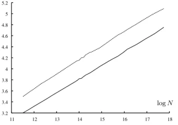
some constant A1, and E( eT1) ≈ log(N )/(ρ + 2). Figure 2
shows the graphs log(E(eν1)) and E( eT1) versus log(N ): the
straight lines depicted prove a good agreement with the the-ory. Moreover, via a fitting procedure, one can compute the slopes of these lines: the results are summarized in Table 1. The values of interest in Table 1 are in the row labeled “Min”: we see that simulations exhibit a slope of 0.248 for eν1
and of 0.256 for eT1, whereas the theory predicts 0.25 in both
cases (because ρ = 2). These results are in good agreement with Approximation 1, which justifies the fact that we can use this approximation up to time eT1.
3.2 3.4 3.6 3.8 4 4.2 4.4 4.6 4.8 5 5.2 11 12 13 14 15 16 17 18 log N
Figure 2: log(E(eν1)) (solid) and E( eT1) (dashed), ρ = 2.
Table 1: Coefficients of growth rates of Fig. 2 and 3 in the case ρ = 2
Policy νe1 Te1 eν2 Te2 νe4 Te4
Min 0.2478 0.2565 0.3765 0.5146 0.3149 0.3287
Random 0.2470 0.2575 0.3711 0.5078 0.2383 0.2530
6.2 Accuracy of Urn and Ball Models
In this section, we compare the random and determinis-tic urn and ball models with E( eT2), the expected value of
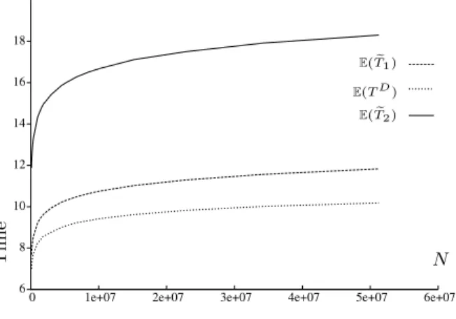
the last time when there is an empty server. It clearly ap-pears in Figure 1 that eT2 closely corresponds to the shift
in equilibrium of the system, and this fact has been ob-served in numerous simulations. However, as we will see in the following, Approximation 1 does not hold until time eT2,
which explains why it is very challenging from a mathemat-ical point of view to derive results on eT2. (Note in addition
that eT2 is not a stopping time).
Figure 3 shows that eT1 is much smaller than eT2: This
result is nevertheless not surprising. Indeed, as discussed in Section 2, results obtained for the random model point out a local behavior: the first empty urn arrives in a region, where still many peers arrive in each interval. Although many peers should arrive in this time interval, this is in reality not the case because a very small interval is generated. Thus, in some sense, the order of magnitude N1/(ρ+2)provided by
the random urn and ball model is misleading for the initial system.
In the deterministic model, the sizes of urns are not ran-dom, and the stochastic fluctuations arising in the random model do not occur. The deterministic model smooths the local behavior that appears in the random model, and the order of magnitude (N/ log N )1/(ρ+1)gives more insight into
the global situation of the system. When only a few peers arrive in an interval, it really means that the equilibrium begins to shift. One can check in Figure 3 that the theo-retical result TDdefined by Equation (20) predicted by the
6 8 10 12 14 16 18
0 1e+07 2e+07 3e+07 4e+07 5e+07 6e+07
E( eT1) E(TD) E( eT2) T ime N
Figure 3: The times E( eT1) ≤ E( eT2) and E(TD) when
ρ = 2.
Although considering the deterministic model indeed im-proves the approximation, eT2 still seems much larger that
TD. However, thanks to our urn and ball models, we know
that the first order approximation of the times eTiis
logarith-mic, whereas the first order approximation for the indexes e
νiis polynomial. Table 1 provides useful information to
un-derstand the situation.
First, the deterministic model yields a reasonable esti-mate of the exponent in eν2: simulations give 0.376 and the
deterministic model 0.333. Note that the random model predicts 0.25, so a substantial improvement in accuracy is obtained when using the deterministic model. This suggests that Approximation 1 holds until TD, i.e., up to times of
order N1/(ρ+1).
Second, we observe a significant discrepancy between the exponent for eν2and the coefficient of eT2: If Approximation 1
were to hold until eT2, one would have eT2≈Peν12Ek1/k, which
would yield, because eν2 ≈ N0.38, that eT2 ≈ 0.38 log(N).
However, we find that the time eT2 is better approximated
by 0.52 log(N ), and so Approximation 1 does not hold until time eT2. This clearly poses the challenge to derive
asymp-totic results for eT2. Moreover, this triggers another
inter-esting question: For how long does Approximation 1 hold? We give a partial answer to this question by considering the times eT3and eT4 in the next section.
6.3 On the Duration of Approximation 1
Throughout this paper, we have tried to estimate the time when the equilibrium of the system begins to shift. As long as Approximation 1 holds, the input rate i(t) of the system is the number of peers, that are not active at time t, times ρ, while the output rate o(t) is just the number of servers at time t (since the service has mean one). Initially, i(0) = ρN and o(0) = 1, and i(∞) = 0 and o(∞) = N . To study the time at which the equilibrium of the system begins to shift, it is therefore very natural to consider the first time
e
T3 at which i(t) < o(t), i.e., when the number of servers is
greater than ρ times the number of non-active peers. As shown in the following, considering this time leads to the order of magnitude given by the deterministic model (with less precise asymptotics of course).
For times t < eT3, we assume that Approximation 1 holds,
so that we can cast eν3 in terms of our urn and ball
prob-lem. Let Zx
N be the number of balls that fall in the x first
intervals: ZNx = x X i=1 ηi(N ) = N X i=1 1 {Eiρ≤Tx}.
The index ν3then corresponds to
ν3= inf x : N − ZNx def = eZNx < x ρ ff . The asymptotic behavior of E`Zex
N
´
when x goes to infinity with N is easy to derive:
E`ZeNx´= N X i>x+1 EPi∼ αN X i>x+1 i−ρ−1∼α ρN x −ρ Therefore E` eZx N ´ ≈ x for x ≈ N1/(ρ+1), i.e. eν 3 is of order
N1/(ρ+1), which is the same order of magnitude as in the
deterministic model. Rigorous mathematical analysis could be done to prove this result, but in our view, considering eT1
has one main advantage: Proposition 1 is almost a rigorous justification of Approximation 1. When considering another time, in particular eT3, we were not able to provide such a
strong justification. And as we have seen in the case of eT2,
Approximation 1 does not hold for the whole first regime, and a strong justification as Proposition 1 is therefore very valuable.
Finally, let us give some brief results on eT4, the first time
when a server empties. Simulations show that eν4 and eT4
have similar behavior as before (polynomial and logarithmic growths, respectively). Results in Table 1 show that the slope for eT4is similar to the exponent of eν4, suggesting that
Approximation 1 holds until eT4.
In conclusion, Approximation 1 holds at least until N1/(ρ+1),
which corresponds to eT1 and eT3. However, it does not hold
until eT2, whereas Figure 1 shows that until eT2, the system
is still in the first regime. For the particular value ρ = 2, we have νD≈ AN0.33
and simulations show that eν2≈ A2N0.38,
and so our approximation by the means of a urn and ball problem is not so far from the exponent that we want to capture. Proposition 1 shows that until νD, there are only
few empty servers: so between TD and eT
2, it could happen
that there is a fraction of empty servers, and although this fraction is small, it has an impact on the system. Similar phenomenon have been observed in Sanghavi et al. [15].
To conclude this section, we discuss a different routing policy. Throughout this paper, we have considered the pol-icy where an incoming peer selects the least loaded server, in terms of number of peers. This policy is compared against the random one, where an incoming peer selects a server uniformly at random among all possible servers.
Simulations show that these policies are very close as shown in Figures 4, 5 and 6. The only noticeable difference is con-cerning E(eν3), cf. Figure 7. However, Table 1 shows that
the exponents of E(eν3) are very similar in the random and
in the minimum policy. One can easily check that they are indeed proportional one to another.
Table 1 shows that for the first time when a server be-comes empty, the policy has a great influence. This is easily understandable: In the min case, it is much harder for a server to become empty, because least loaded servers are selected by incoming peers.
6.5 7 7.5 8 8.5 9 9.5 10
2e+06 6e+06 1e+07 1.4e+07 Min
Random
T
ime
N
Figure 4: Comparison of Min and Random for E( eT1)
when ρ = 2 40 45 50 55 60 65 70 75 80 85
2e+06 6e+06 1e+07 1.4e+07 Min
Random
T
ime
N
Figure 5: Comparison of Min and Random for E(eν1)
when ρ = 2
7. CONCLUSION
The simulations moreover underlined the existence of a second regime during which although the fraction of idle servers is small, the output rate is no longer as high as pos-sible. This second regime is then followed by a third regime during which the capacity offered by the system exceeds by far the input rate, and so the system mainly creates empty servers. Our urn and ball approach can no longer be applied to these two regimes, and so they will be studied in the near future using other probabilistic techniques.
A possible extension of our results consists of incorporat-ing the possibility for a peer to leave the system right after completing its download. In terms of urn and ball, this just amounts to change the parameter that defines the length of the n-th interval: instead of n, one would just have to con-sider pn if p is the probability for a peer to become a server after completing its download. An extended model where the file is split into different chunks essentially amounts to study a multi-class queueing network with a random num-ber of servers of different classes which proves to be a much more difficult problem.
Finally, a natural extension is to consider a general service distribution, instead of the exponential one. In this case, the process of creation of servers can be described as a binary Bellman-Harris branching process. See Athreya [2, 3]. If this setting complicates significantly the analysis of the file sharing system, it seems that most of the results obtained in the exponential case should still hold.
14 14.5 15 15.5 16 16.5 17
2e+06 6e+06 1e+07 1.4e+07 Min
Random
T
ime
N
Figure 6: Comparison of Min and Random for E( eT2)
when ρ = 2 200 300 400 500 600 700 800 900 1000
2e+06 6e+06 1e+07 1.4e+07 Min
Random
T
ime
N
Figure 7: Comparison of Min and Random for E(eν2)
when ρ = 2
8. REFERENCES
[1] Søren Asmussen, Applied probability and queues, John Wiley & Sons Ltd., Chichester, 1987.
[2] K. B. Athreya and Niels Keiding, Estimation theory for continuous-time branching processes, Sankhya: The Indian Journal of Statistics 89 (1977), no. A, 101–123. [3] Krishna B. Athreya, On the supercritical one
dimensional age dependent branching processes, The Annals of Mathematical Statistics 40 (1969), no. 3, 743–763.
[4] A. D. Barbour, Lars Holst, and Svante Janson, Poisson approximation, The Clarendon Press Oxford University Press, New York, 1992, Oxford Science Publications.
[5] F. Cl´evenot and P. Nain, A simple fluid model for the analsysis of the Squirrel peer-to-peer caching system, Proc. Infocom, 2004.
[6] E. Cs´aki and A. F¨oldes, On the first empty cell, Studia Scientiarum Mathematicarum Hungarica 11 (1976), no. 3-4, 373–382 (1978).
[7] Z. Ge, D.R. Figueiredo, S. Jaiswal, J. Kurose, and D. Towsley, Modeling peer-to-peer file sharing systems, Proc. Infocom, 2003.
[8] Alexander Gnedin, Ben Hansen, and Jim Pitman, Notes on the occupancy problem with infinitely many boxes: general asymptotics and power laws,
Probability Surveys 4 (2007), 146–171 (electronic). MR MR2318403
[9] Bronius Grigelionis, On the convergence of sums of random step processes to a poisson process, Theory of Probability and its Applications 8 (1961), no. 2, 177–182.
[10] Hsien-Kuei Hwang and Svante Janson, Local limit theorems for finite and infinite urn models, Annals of Probability (To appear).
[11] J. F. C. Kingman, Random partitions in population genetics, Proceedings of the Royal Society. London. Series A. Mathematical, Physical and Engineering Sciences 361 (1978), no. 1704, 1–20.
[12] Unpublished manuscript available at, http://chambertin.inria.fr/robert/Sigmetrics-Theorem2.pdf.
[13] L. Massouli´e and M. Vojnovi´c, Coupon replication systems, Proc. Sigmetrics 2005 (Banff, Alberta, Canada), June 2005.
[14] D. Qiu and R. Srikant, Modeling and performance analysis of BitTorrent-like peer-to-peer networks, Proc. Sigcomm, 2004.
[15] Sujay Sanghavi, Bruce Hajek, and Laurent Massouli´e, Gossiping with Multiple Messages, INFOCOM 2007. 26th IEEE International Conference on Computer Communications. IEEE, May 2007, pp. 2135–2143. [16] David Williams, Probability with martingales,
Cambridge University Press, 1991. [17] Xiangying Yang and Gustavo de Veciana,
Performance of peer-to-peer networks: service capacity and role of resource sharing policies, Performance Evaluation 63 (2006), no. 3, 175–194.