Viscous modified chaplygin in classical and loop quantum cosmology

People's Democratic Republic of Algeria Ministry of Higher Education and Scientific Research

University of the Mentouri Brothers of Constantine Faculty of Exact Sciences

Department of Physics

No _{of order:}

No of series:

Thesis

To obtain the degree of

Doctorate Third Cycle in Physics

Specialty

Theoretical Physics

Subject

Viscous Modified Chaplygin in Classical and Loop

Quantum Cosmology

Presented by

Dalel Aberkane

Members of jury:

President M. A. Benslama Professor University of the Mentouri Brothers Supervisor N. Mebarki Professor University of the Mentouri Brothers Examiners H. Auissaoui Professor University of the Mentouri Brothers

M. Boussahel Professor University of M‟sila S. Zaim Batna Professor University of Batna

i

Contents

Acknowledgements vi

Introduction v

Chapter one: classical cosmology

1. FRW cosmology

1.2 The Einstein field equations………...2

1.3 The Robertson walker metric………...4

1.4 The energy momentum tensor………....5

1.5 Bulk and shear viscosity……….7

1.6 Cosmological models in standard cosmology……….…..8

1.7 The big bang singularity and inflation………...10

1.8 Modeling dark energy and dark matter……….…13

2

. Cosmological measurements

2.2 The proper distance and particle horizon………..14

2.3 The red shift parameter……….…15

2.4 The Hubble‟s law………. ………...16

2.5 Luminosity distance………...17

2.6 Distance modulus………...18

ii CONTENTS

Chapter two: loop quantum cosmology

1.

1.1 Why we need to quantize gravity?...21 1.2 Why loop quantum gravity?... ...22

2. The Hamiltonian formalism of GR

2.1The Hamiltonian formalism of a classical theory……….23 2.2 The ADM formalism………....24 2.3 The Hamiltonian formulation of GR………....26

3. The Platini formulation of GR

3.1 The tetrad formalism……….…………31 3.2 The ADM formalism on the tetrad……….………..33

3.3 The Ashtekar‟s variables……….………..………...33

4. Isotropic loop quantum cosmology

4.1 Why holonomies?... 36 4.2 Holonomy-flux algebra……….………36 4.3 The modified Friedman equation ……….…....37

Chapter three: Modeling Dark Energy by VMCG

1. Viscous Modified Chaplygin Gas Model

1.1 Chaplygin Gas Models………...42 1.3 A VMCG dominated universe ……….…...44

2. Constraining VMCG in Standard Cosmology

iii

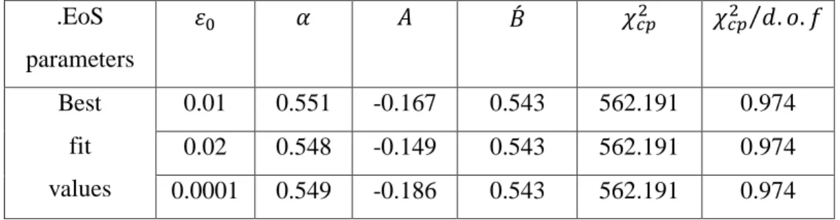
2.2 The Best Fit values of the EoS parameters of VMCG model………...50

2.3 Cosmological parameters in terms of the Best Fit values of the EoS parameters……..56

3. Dynamical analysis of VMCG in LQC

3.2 The Autonomous System of VMCG in LQC………..…...62

3.3 Numerical analysis………...………..66

Conclusion

vi CONTENTS

Acknowledgements

First of all, I am grateful to the Almighty God for establishing me to complete this work. The completion of this thesis would not have been possible without the guidance, support and

expertise of Prf. Mebarki Noureddine, my honorable thesis supervisor. I would also like to thank the committee members Professors: M. A. Benslama, H.

Auissaoui, S. Zaim, M. Boussahel, for checking this study and for oral examination who manifested their distinguished skills in their own fields as seen in their way of correction and

ideas shared.

It would not have been possible to write this doctoral thesis without the help and support of the kind people around me, to only some of whom it is possible to give particular mention

here.

I would like to express my gratitude to my parents, sister Romeissa who have given me their unequivocal support throughout, as always, for which my mere expression of thanks likewise

does not suffice.

My joy knows no bounds in expressing my cordial recognition to my best friends Boukhlouf

Sara, and Benchikh Sara. Their keen interest and encouragement were a great help

throughout the course of this research work.

I‟m deeply indebted to my respected teachers and other members of Physics department in Batna and Constantine, for their invaluable help.

A sincere gratitude to the Subatomic and Mathematical Laboratory of Mentouri University.

v

Introduction

One of the most intriguing questions in modern physics is the fundamental machinery behind the accelerated expansion of the universe. With recent observational data coming from Type Ia Supernovae [1,3], cosmic microwave background anisotropies[4−6] and large galaxy surveys[7,8] , the misleading conception of a static universe is abandoned for a universe that is in an accelerated motion where stuff are constantly taking away from each other. This discovery has shed light on a new research era in aim to explain the physics

behind this motion. Different answers was brought to the arena and structured mainly into two different approaches: the first one treats general relativity as incomplete theory that needs to include modifications in aim to predict the accelerated expansion. In different words, the accelerated expansion should be inherently related, at large scale limit, to the geometry of a modified theory of gravity. The second one takes more seriously the Einstein‟s theory in a way that it should be fully trusted, so the accelerated motion is derived by adding a new exotic component of the universe with a negative pressure called dark energy [9,10]. If we follow the second path, especially that the theory is well tested at large scale, the existence of a new physical object filling the universe will rise several questions about its fundamental structure and how it couples with other stuffs in the universe. Although, different models were proposed involving baryonic and non-baryonic candidates [11,12], we still don‟t know which one describes the reality the best, models are subject to verifications through recent

iv CONTENTS One of the well accepted models are the Chaplygin gas models, they were widely scrutinized and modified since they were first proposed. They are combined models that unify both dark energy and dark matter and give a suitable negative pressure that drives the acceleration of the universe. The Chaplygin gas was first proposed as a dark energy model in [13]. Although, its equation of state was generalized [14] to fit with observational data, at high energy density the Generalized Chalpygin Gas (GCG) mimics dust with ( ) and suffers from instabilities at the perturbative level [15]. Therefore, Modified Chaplygin Gas (MCG) was proposed by adding a further modification to the GCG. Its EoS parameters were also constrained using different observational data [16-19].

Similarly, viscous modified Chaplygin gas (VMCG) with the generalized EoS was

investigated in Ref. [20], as it is possible to assume that the expansion process is a collection of states out of thermal equilibrium that gives rise to bulk viscosity. A variety of bulk

cosmological models have been explored by several researchers [21-26].

Unfortunately, classical models suffer from early and late time singularities. Those can be avoided in the framework of loop quantum cosmology (LQC) [27-31] which is a non-perturbative and background-independent type of quantization of gravity [32,33] used to probe some cosmological problems. In addition of predicting an inflationary phase of the early universe [34-37] and late time cosmic acceleration[38], the semi-classical approximation in LQC formalism can be validly used at late time and at large scale [39].

As the MCG was found to be consistent with the evolution of the universe over a wide range of epochs [40] and it is preferred by recent observational data because of its small minimum

value [16] and as the universe throughout its evolution might gave rise at its beginning to bulk viscosity, we chose VMCG with a specific bulk viscosity pressure to model the dark content of the universe and explore the model‟s behavior at present time when fitted to recent observational data, its fate at late time and whether it suffers from singularities or not.

First, we constrained its Eos parameters using Union 2.1 data for a suitable model that describes the current universe. We also evaluate cosmological key parameters at present and early universe and determine their present values to deduce if the model is consistent or not with observational data and theoretical predictions. The values are compared to those of other well accepted models. Then, we probe the dynamical behavior of the model at early and late time in the LQC framework especially as the model suffers from the Big Bang singularity.

v This thesis is organized as follows:

In the first chapter we explore the FRW cosmology along with some cosmological models derived from it. The bulk viscosity is also introduced when fluids describing stuff in the universe are no longer perfect. This is followed by exposing some flaws within the classical cosmology. Then, we define some important parameters used for cosmological

measurements.

In the second chapter we begin by giving an overview of the motivation behind a quantum theory of gravity and loop quantum gravity as a special case. Then, the mathematical formalism inherent to the theory is introduced and the main ideas behind every step toward this formalism are explained. The modifications on Friedmann equations due to loop quantum cosmology corrections are illustrated.

In the last chapter, some of the Chaplygin gas models are explored briefly before introducing the VMCG model and the formula chosen for the bulk pressure. Then, we started by solving analytically the conservation equation of a VMCG dominated universe to check the behavior of the solution at early, present and late time. The model is constrained using recent

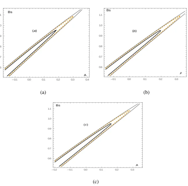
observational data, we used Mathematica to calculate the best fit parameters and draw the contour plots of some confidence levels. The behavior of the model is then probed at small and present scale using the time evolution of cosmological parameters. Finally, in LQC framework, the dynamical analysis is conducted using Maple and Mathematica.

1

Chapter one:

Classical Cosmology

“We cannot solve our problems with the same

thinking we used when we created them”

CHAPTER ONE . CLASSICAL COSMOLOGY

2

1 FRW Cosmology

1.1 The cosmological principle

It states that the universe is large enough (level of clusters of galaxies) to assume that all points of the universe are equivalent which

means that the universe is assumed to be homogeneous and isotropic around any point.

Homogeneous: there is an isometry (a transformation that preserves distance relationships) that can carry any vector to a nearby point, so the geometry is the same at any point as it is at another.

Isotropic: if you rotate around a point the space looks the same without any preferred direction.

1.2 The Einstein field equation

According to Newtonian gravity, gravitational mass is the only source of the gravitational field but with both energy-mass equivalence and equivalence principle,

gravitational field couples in the same way mass and energy and they are both described by the same mathematical entity called the energy-momentum tensor . The space used to describe the theory of general relativity is not the 3-dimensional Euclidean space of Newton mechanics and the second derivative in the Euclidean space is replaced by the curvature (Ricci) tensor in the Riemannian space so

Newtonian Gravity General Relativity

1 FRW COSMOLOGY

3 In its field equation, Einstein established a relationship between the energy density content of the universe and the curvature of the space time

(1.1)

where is the Ricci scalar, the metric and the gravitational constant. This equation states that the space-time geometry is dictated by the distribution of energy filling the universe.

The vacuum equation used to study the gravitational field outside the source is called Vacuum Einstein equation and is given by

(1.2)

The problem with Eq. (1.1) is that if the gravitational force (an attractive force) is the only active force at the present scale, the universe will eventually shrink and collapse. As Einstein disliked the idea of a dynamic universe, he added a fudge factor to the equation to completely balance the attractive force and made the universe closed, homogeneous and static.

(1.3)

Where is the cosmological constant.

In 1920s, Wirtz and K. Lundmark showed that Siphers‟s red shifts increased with the distance of the nebulae, and in 1929, Hubble established a linear relation between distances and

velocities so the furthest objects are the fastest [41]. Therefore, the universe is not static and rather in an accelerated motion, this fact forced Einstein to admit that the added factor is his biggest mistake. The infinite structure of the universe is no longer a problem if we assume that the cosmological constant is the vacuum energy.

1.3 The Robertson-Walker metric

As the universe is assumed to be homogeneous and isotropic, the metric describing how lengths are measured in this space should include those two conditions.

CHAPTER ONE . CLASSICAL COSMOLOGY

4 The geometry of such a space is spherically symmetric about a point and can be described using the Schwarzschild metric for a static gravitational field

_(1.4)

The metric has no preferred angular direction and is time-independent (no mixed terms). Taking into account the fact that an observer at a fixed point moves only forward in time along a geodesic which is parallel to the time coordinate line we have

(1.5)

As the universe is dynamic the metric can be written as

_(1.6)

Where is the scale factor that describes how the size of the universe evolves in time. Using the fact that in spatially isotropic and homogeneous space the curvature of the space is constant and is related to the Riemann tensor [42] we find the R-W metric

(1.7) Where is the normalized curvature constant.

Positive curvature : the surface is a two sphere (a closed space) where the sum of the angles of a triangle on this surface is greater than 180⁰.

Negative curvature : the surface has an infinite volume (an open space) where the sum of the angles of a triangle on this surface is less than 180⁰.

1 FRW COSMOLOGY

5 Zero curvature : a flat space where the sum of

the angles of a triangle on this surface is equal to 180⁰.

1.4 The energy-momentum tensor

According to the general covariance principle, all invariant laws in physics under coordinate transformation should be stated in tonsorial form. Similarly, any distribution of matter or energy as a source of the gravitational field should be stated in terms of the energy-momentum tensor as energy is an invariant quantity under coordinate transformation.

We consider a momentum and an energy that are contained in an infinitesimal volume so the momentum 4-vector is proportional to the volume [42] by

_(1.8)

Where _{is the factor of proportionality, called the energy-momentum tensor. It is the flux}

of the component of the momentum 4-vector across the surface defined by a constant .

_{: is the energy density defined as the flow of the energy through a surface of a constant}

time.

_{: is the energy flux defined as the flow of the energy through a surface of a constant . : is the momentum density defined as the flow of the momentum through a surface of a}

constant time.

_{: is the stress defined as the flow of the momentum through a surface of a constant}

CHAPTER ONE . CLASSICAL COSMOLOGY

6 The conservation equation:

The conservation equation of the energy momentum tensor is given by

_(1.9)

Where is the covariant derivative. Energy-momentum tensor of dust:

Dust is defined as a perfect fluid with non-interacting and non-relativistic particles with no pressure, moving together with some velocity so they carry energy and momentum as a source of a gravitational field.

The energy-momentum tensor for dust is given by

_(1.10)

Where is the energy density of dust particles, is the velocity 4-vector of dust particles in the chosen frame.

Energy-momentum tensor of a perfect fluid:

A perfect fluid is defined as a fluid where any region nearby a co-moving observer with the fluid is seen to be homogeneous and isotropic so all the directions for a co-moving frame are equivalent. In such a fluid there is no heat flow or viscosity and the changes within the fluid are only adiabatic. The energy-momentum tensor of such a fluid is given by

_(1.11)

Where is the pressure of the perfect fluid, is the energy density of the fluid, _{is the}

metric of the space.

Energy-momentum tensor of a generalized fluid:

The general form of energy-momentum tensor of a more complicated fluid [42] is given by

_(1.12)

Where : specific energy density of fluid in its rest frame, _{: the spatial}

1 FRW COSMOLOGY

7 lines, :the acceleration tensor, : shear viscosity, _:

shear tensor, : the energy flux tensor.

1.5 Bulk and shear viscosity

Shear viscosity of a fluid measures how strong is the couple between different layers of the fluid of the same velocity under a shear stress (the friction between two layers with different velocities)

(1.13) Where is the stress tensor, shear viscosity and the velocity gradients. The stress in this case is not provoked by velocity but by the change of velocity from point to another. In case of incompressible fluids (flow velocities ˂˂ the speed of sound) the divergence of the velocity vanishes.

Bulk viscosity deals with compressible fluids (flow velocities ≈ the speed of sound) where the divergence of the velocity is non-vanishing and induces an extra dynamic pressure

(1.14) Where is the bulk viscosity. As it is noticed, the dynamic pressure is negative in regions where the fluid expands . The general form of the stress tensor will be given by

( ) (1.15)

Where is a constant, is the pressure of the fluid taken as the average of the three normal stresses ∑ defined by

(1.16) Where is the equilibrium pressure given by the state equation , so the stress tensor can be written as

( ) (1.17)

Viscosity may arises from a number of dissipative processes in the early universe such as the decoupling of matter and radiation era, the inflationary phase, formation of galaxies,..etc.

CHAPTER ONE . CLASSICAL COSMOLOGY

8 Universes that are assumed to be isotropic and homogeneous are shearless and only bulk viscosity is taken into account. Bulk stress at late time may induce a negative pressure that drives the acceleration of the universe. This viscosity might be attributed to a fluid describing matter or dark energy. Eckart [43] made the first attempt to describe a relativistic theory of viscosity with the bulk pressure

(1.18) in which is the bulk viscosity and the Hubble parameter.

1.6 Cosmological models in standard cosmology

Standard cosmology is a class of dynamical cosmological models characterized by a

homogeneous and isotropic distribution of stuff in the universe, such models have a universal time which is non-common in relativity.

We model matter and energy by a perfect fluid energy-momentum tensor then we solve Eq. (1.1) using the RW metric and find the Freidmann equations [44]

̇ (1.19)

̈ _{̇ (1.20)}

Solving the conservation equation of the energy-momentum tensor _gives

̇

(1.21) This result corresponds to the first law of thermodynamics .

Friedmann equations gives rise to different possible models, we only state some of them as the following:

Radiation dominated universe:

The early universe was dominated by radiation or an extremely relativistic gas with non-interacting particles, radiations are modeled as a perfect fluid where the state equation is given by

1 FRW COSMOLOGY

9 Where and are respectively the density and pressure of radiations, replacing the state equation into the Eq. (1.21) we find

_(1.23)

So as the universe is expanding, the radiation density drops faster than matter because of the redshift effect on photons.

Matter dominated universe:

Matter represents all the non-relativistic stuff of the universe considered as a source of the gravitational field, it is modeled by dust . With the expansion of the universe, matter density decreases with a factor of

_(1.24)

As the density of radiation drops faster than matter within the expansion process the universe gets colder and becomes dominated by matter.

In the above two models, we have a decelerated expansion but it is more rapid in a universe dominated by radiation with √ as it is in a universe dominated by matter with ⁄ _{, this is due to the pressure of the radiation.}

Vacuum dominated universe:

When we drain the universe from its content (all matter and radiation) we are left with a vacuum energy that can be modeled by the cosmological constant with

(1.25)

or by a perfect fluid with negative pressure with equation of state

(1.26) where is the required state parameter to drive an accelerated expansion of the vacuum dominated universe.

CHAPTER ONE . CLASSICAL COSMOLOGY

10 In FRW cosmology De-Sitter universe corresponds to a homogenous and isotropic vacuum dominated universe with a positive cosmological constant and a positive curvature. The accelerated expansion in this universe is exponential

_(1.27)

1.7 The Big Bang singularity and Inflation

When the early universe was dominated by radiation with ), it was found to be in a decelerated expansion which means that if we keep going back in time the universe will be shrinking till will reach a singularity point at called the “initial” or the “Big Bang” singularity.

The idea of a singular origin of the universe was firstly proposed by Lemaitre, a catholic priest who worked on the theory of general relativity and the origin of the universe.

According to his ethnic beliefs, the universe was created from a “cosmic egg”. Nevertheless, as he was not capable to develop further this idea, he has not been taken seriously. In the 1940s, R. Alpher and G. Gamow assumed that the universe at its beginning was hot and dense enough to allow the creation of helium, lithium, deuterium and later hydrogen, and in 1960, the astronomer Fred Hoyle came up with the name “Big Bang”.

From this singularity point the universe is assumed to be created, it can be predicted by the singularity theorems where every universe with ) must have begun at a singularity.

As we have a density that increases and a temperature that goes to infinity , in this case classical theory of relativity is not capable of describing the physics in the vicinity of this singularity. A quantum theory of gravity is needed to solve this problem.

Even if the Big Bang model gave successful predictions on Cosmic Microwave Background (CMB) radiations, the abundance of light elements and the Big Bang nucleosynthesis, several problems are embodied in this model, for example dark energy and dark matter are not

described by this model, likewise, CMB radiations have been observed in different directions, for points that are not in causal contact, with surprisingly uniform results. This is called the Horizon problem.

1 FRW COSMOLOGY

11 Another problem arises where recent observations set the density parameter of the present universe to , this result implies the flatness of the universe as , because any weak deviation from at implies a great deviation from unity at the present time. How can we explain the steadiness of this equality along the evolution of the universe?

The prediction of the existence of magnetic monopoles created in the hot early universe is another problem of this model because no observational evidence of their existence has been made yet.

All these problems and others were solved in the context of an inflationary theory.

The first simple model describing an inflationary period was proposed by Alan Guth in 1981 called the “old inflation”, it was based on an exponential expansion of the universe in a super-cooled false vacuum state (a state without any particles or fields but with large energy

density). This model didn‟t work and was replaced by a new inflationary model in 1981-1982, however, both were considered as incomplete modifications of the Big Bang model. In 1983, a chaotic inflation scenario was proposed to solve problems of the old and new inflation. We consider that the very early universe was filled with a scalar field called “inflaton” with a mass and a potential energy density . The Einstein equation for a

homogeneous universe filled with the inflaton is given by

̇ (1.28) Where is the curvature constant, the dot stands for the derivative with respect to the cosmic time.

Because of the expansion of the universe the equation of motion of the scalar field coincides with equation for harmonic oscillator

̈ ̇ (1.29) If is large initially then from Eq. (1.27) and the friction term ̇ from Eq. (1.28) are large too. This means that the scalar field is moving slowly and maintains an almost constant energy density when the universe is expanding rapidly, so we have at the very beginning

CHAPTER ONE . CLASSICAL COSMOLOGY

12 This leads to a slow change in and an exponential expansion of the universe with

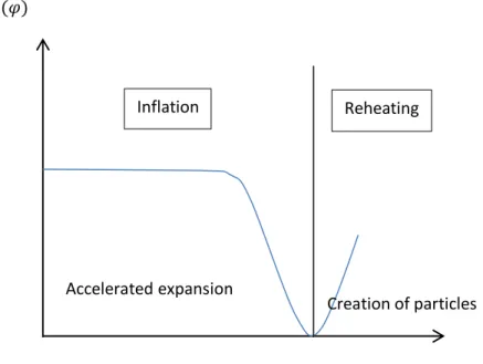
√ _(1.31) For small values of called also the slow-roll potential, the inflaton moves slowly down as a ball in a viscous liquid [45].

Figure 1.1: At the minimum of , the inflationary period comes to an end and the scalar

field rapidly oscillates, the universe enters a reheating period where pairs of elementary particles are created from the scalar field .

The inflation period is so rapid, for example, in one of the inflationary models it is

approximately 10-30s during this time the universe expands from 10-33cm the Plank size to

cm. Those numbers are model-dependent but the size of the universe always gain in many orders of magnitude compared to its initial size and compared to the actual horizon size _{cm, that is the part of the universe that we can see now. In fact, this property is the key}

solution to both horizon and platitude problems, so even if the universe is initially closed after inflation the distance between its both poles is greater than _{cm which means that the}

visible universe looks flat. Similarly, neighboring points in causal contact before inflation will be driven apart in different directions during inflation with a speed greater than the speed of light which gives a plausible explanation to CMB observations and the horizon problem.

Inflation Reheating 𝑉 𝜑

𝜑 Accelerated expansion

1 FRW COSMOLOGY

13

1.8 Modeling dark energy and dark matter

Recently, Type Ia Supernovae observational data[1−3] with cosmic microwave background anisotropies[4−6] and large galaxy surveys[7,8] have shown that the universe is undergoing an accelerated expansion phase. The mysterious force or energy leading to the accelerated expansion was attributed to:

1- Vacuum as a vacuum energy with some exotic properties called “dark energy”. 2- An asymptotic behavior of a modified theory of gravity at the cosmological scale. A theory of a modified Newtonian dynamic (MOND) that can solve the problem of the velocity anomalies without the need of a concept of dark energy.

3- Signature of extra-dimensions.

Following the first stream of ideas, the existence of an exotic kind of energy, called dark energy, with negative pressure that drives the universe to expand was proposed and is modeled by several candidates:

1- The cosmological constant with

2- Dark energy as a perfect fluid with the equation of state , 3- Dynamical dark energy with

4-

Astronomers have long known that galaxies and clusters would fly apart unless they were held together by the gravitational pull of much more material than we actually see. The argument that clusters of galaxies would be unbound without dark matter dates back to Zwicky (1937) and others in the 1930s. A wide range of different candidates for dark matter were considered. The first suggested were baryonic, consisting of three quarks , candidates in this category were ionized gas, very faint, low-mass stars and collapsed objects, like stellar black holes. Non-baryonic candidates were also proposed, like neutrinos. MOND is another alternative to dark matter in which the theory of gravitation requires modification without the need to postulate the existence of dark matter [46].

CHAPTER ONE . CLASSICAL COSMOLOGY

14

2 Cosmological measurements

2.1 The comoving coordinate system and the cosmic time:

Let us imagine in a region of space particles that are free falling carrying a coordinate system and a clock so the event line between two events of a moving particle will be simply seen as the proper time that collapses between the two events (purely temporal)

(1.33) This means that . We also, have a trajectory that satisfies the free falling equation

(1.34)

which leaves us with .

The coordinate system that satisfies Eq. (1.33) and (1.34) is called Gaussian.

In the comoving coordinate system the observer is moving with the Hubble flow, in other terms the observer expands with the universe expansion, for such an observer the universe is isotopic.

The cosmic time is the proper time of a local observer for whom the local material of the universe is on the average at rest [42].

2. 2 The proper distance and particle horizon

The distance between two galaxies at and with same angle coordinate is the cosmic time it takes light to travel from to

⁄ (1.35)

The proper distance between two galaxies at and at a fixed cosmic time is ∫

2 COSMOLOGICAL MEASUREMENTS

15 The partical horizon is the largest value of from which we could have received at the present time a light signal emitted at the earliest possible time.

∫ ∫

⁄

(1.37)

2.3 The redshift parameter

a signal emitted at from arrived at

∫ ∫

⁄ (1.38)

another signal emitted at from arrived at ∫

∫

⁄ (1.39)

As the change in the scale factor is very insignificant during this period we find

(1.40)

Where and are the period of light received and emitted. Now, we can write

(1.41)

Where and are the wave length of the first and the second signals. Depending on how space is evolving in time (expansion or contraction) during the transit of a signal of light we can have either a red shift result or a blue shift result.

Several astronomical observations in1920‟s showed that then which means a redshift result and the fractional increase in the wave length is given by the redshift parameter

CHAPTER ONE . CLASSICAL COSMOLOGY

16

Figure 1.2: As the universe is expanding the wavelength of a signal of light travelling from

(1) to (2) is stretched out.

For nearby galaxies where and are small and we have

̇ ̇ ̇ (1.43) Where is the proper distance and the dot stands for the derivative with respect the cosmic time. The redshift parameter here is due to the Doppler shift for low relative velocities ̇ between the observer and the emitter [42].

2.4 The Hubble’s law

The Hubble‟s law states that the distance of a (nearby) galaxy from us is related to its velocity [41]. For nearby galaxies, so we have

̇ ̇ (1.44)

From (1.40) we can write

̇ (1.45) Where ̇ is the Hubble‟s constant.

The Hubble parameter is defined as the rate of expansion of the universe and is given by

2 COSMOLOGICAL MEASUREMENTS

17 There is a great uncertainty on its present value called the Hubble constant and given by (sec-1or Km/sec/Megaparsecs).

The Hubble time is a time scale for the present universe and at a given Hubble time all galaxies in the universe are located at the same point.

2.5 Luminosity distance

The luminosity of a galaxy is defined as the total power of radiation emitted per unit time and is related to the flux by

(1.47) Where is the luminosity distance and is given by

(1.48) Where and are the time when the light signal is emitted and received from a galaxy at , for nearby galaxies .

Since is not an observable quantity and we need to replace it by an observable quantity, we begin by expanding the redshift parameter in power series of for galaxies not far away we find

( ) (1.49) Where is the present deceleration parameter, then we use Eq. (1.30) to expand we find

(1.50)

Hence the distance luminosity will be given by

(1.51)

Therefore, the measurement of the luminosity distance and the redshift of a sufficient number of galaxies we can determine both and in a good approximation [47].

Different methods are used to measure the distance luminosity and every method has its own limits in terms of precision, type of galaxies and the range of the distance scale. One of them

CHAPTER ONE . CLASSICAL COSMOLOGY

18 consists of finding what astronomers call “Standard Bulbs”, objects with the same intrinsic brightness wherever they are. The distance luminosity in this case depends only on the apparent brightness; the furthest objects are the faintest. Several suggestions were made including “supergiant stars, planetary nebulae, giant ellipticals and brightest member of a galaxy cluster”. Another interesting candidate is type Ia Supernovae, those objects all reach nearly the same intrinsic brightness (4.5 109 Lsun) and they can be observed in all type of

galaxies, even more, their range of distance scale is over the 8 billion light year.

We recall another useful method that is however used for a range of distance scale less than 110 million light year, in this method the astronomers use the variable stars “pulsating stars” to draw their light curves (the apparent magnitude as a function of time in days) and then deduce the luminosity and the distance luminosity. Candidates for variable stars are Cepheids and RR Lyrae stars. Cepheids are the brightest with a greater period (3-50 days) compared to RR Lyrae stars (less than a day). They were the object of measurements in 1920 by Hubble when discovering the expansion of the universe.

2.6 Distance modulus

The distance modulus is the difference between the apparent magnitude (How bright a star appears in the sky) and the absolute magnitude (How bright a star would appear at 10pc) given by

(1.52) and is related to the luminosity distance by

(1.53) where [47]

2.7 Critical density and the density parameter

As stated before the geometry of the space is determined by the density of things in the universe, and the critical density is defined as the amount of density required to have a flat spatial geometry of the universe

2 COSMOLOGICAL MEASUREMENTS

19

(1.54)

The density parameter is the ratio between the total density of stuff in the universe and the critical density

(1.55) In case of the universe is closed and , in case of the universe is flat with and in case of the universe is open with .

20

Chapter two:

Loop Quantum Cosmology

“

Science never solves a problem without creating ten more”

CHAPTER TWO. LOOP QUANTUM COSMOLOGY

21

1 The motivation behind loop quantum gravity

1.1 Why we need to quantize gravity?

Seventy years ago, was the golden age of new ideas for physics and all the breakthroughs were the result of pushing boundaries and limits of the incomplete theories of that time. At the microscopic scale, a complete set of new ideas were proposed to describe the strange behavior of elementary brakes of matter giving birth to Quantum Mechanics. The new theory is background dependent, non-local and probabilistic, where particles are treated as quanta of fields and fields as quanta of particles and the dynamic of such fields is described through the time evolution of the Hilbert space functions with respect to a space background. Whereas, at the macroscopic scale, General relativity attempts to describe the gravitational force as the deformation of the space-time which means that space-time is not anymore an absolute web structure that witnesses the dynamic of other objects but it is treated as a dynamical object itself. The Einstein‟s new theory is then background independent, deterministic and local so both theories are giving us a schizophrenic understanding of the universe.

May be we need again to push both theories to their limits and explore what happens? Quantum field theory suffers from UV or short distance divergences, the renormalization by introducing a short-cut off allows us to avoid infinities but also comes with price of ignoring the physics of extreme short distances.

General relativity also has its own divergences, Big Bang or black hole singularities where high energy density is confined in a singularity point results in a divergence of the curvature and a breakdown of the geometry.

In both cases, QFT and GR are pushed beyond their limits when describing extreme short distances of space filled with extreme high energy density. The fabric of space-time is no longer continuous and high energy density requires quantum effects which call for a theory of quantum gravity. In this new theory, QFT and GR can coherently coexist to solve the above inconsistencies [48].

2 THE HAMILTONIAN FORMALISM OF GR

22

1.2 Why loop quantum gravity?

The quantization of gravity can be treated in two different ways:

One way is to split the metric into a background Minkowsky metric and a perturbative metric to restore the background notion when quantizing the theory. This approach predicts the existence of extra-dimensions of the space-time along with new particles and may lead to a unified theory of all interactions (string theory, M theory). However, the splitting of the metric violates the background independence, the diffeomorphism covariance and leads to the non-renormalizability of the theory .

Another way to do the quantization without additional structure is the canonical quantization of GR where matter and geometry are unified in a non-standard sense making them both transform covariantly under the diffeomorphism group at the quantum level. This is a background independent, non perturbative type of quantization where the fundamental principles of general covariance and quantum mechanics are combined in a consistent mathematical way. Space-time is treated as a dynamical field, interacting with other fields and quantized like any matter field with no need to any background structure [48-50].

CHAPTER TWO. LOOP QUANTUM COSMOLOGY

23

2 The Hamiltonian formalism of GR

2.1 The Hamiltonian formalism of a classical theory

The dynamic description of a system is defined by its evolution in time. This evolution is encrypted in the Hamiltonian function or density , where are the generalized coordinates of the phase space, the canonical momentum of .

To determine the Hamiltonian density we need first to introduce the Lagrangian density ̇ as a function of the generalized coordinates and their velocities ̇ , it is defined at every point (generalized coordinate) of the trajectory of the system.

The canonical momentum of is then given by

̇

̇ (2.1)

The resulting equations are used to find ̇ . The Hamiltonian density is then defined by

( ) ∑ ̇ ̇ (2.2) which encodes the dynamic of the system and as a result the equations of motions are given by { ̇ ( ) ̇ ( ) (2.3)

For systems where , the Hamiltonian density is the total energy of the system. However, if we have ( ), the third equation of motion in (2.3) is added [51].

2 THE HAMILTONIAN FORMALISM OF GR

24 For a constrained system the resulting equation of motions are

{

̇ ( ) { }

̇ ( ) { } (2.4)

where are the constraints of the system, are arbitrary variables called Lagrange multipliers and the Poisson brackets are defined by

{ } ∑ (2.5)

2.2 The ADM formalism

In aim to describe the dynamics of the gravitational field using the Hamiltonian approach we need first to fix a proper time from which the evolution of the system is carried out. However, general relativity treats space and time on the same footing, and breaking off the space-time into space and time may break the general covariance (the diffeomorphism) of the theory.

Thanks to Geroch‟s theorem, a globally hyperbolic space-time is diffeomorphic to a manifold

(2.6) where a hypersurface of equal time and is a diffeomorphism mapping the space-time manifold to . We recall that diffeomorphism is an isomorphism on a differential manifold.

A globally hyperbolic space-time contains Cauchy surfaces (spatial-like surfaces) as

submanifolds. This is a fundamental requirement because the causality of theory is encoded in Cauchy surfaces where a causal time-like curve intersects the spatial slice only once. A way to see this is to imagine the whole universe at a constant time as a Cauchy surface .

CHAPTER TWO. LOOP QUANTUM COSMOLOGY

25 This feature is very important when formulating the theory as it implies that the behavior of the universe at any time can be derived from initial data of the system. This is dictated by the change of the flow of the time-like curves through space-like surfaces in accordance with Einstein„s field equations.

Now as we divide the space-time into space-like slices crossed by time-like curves, the metric of the space-time will be written in terms of the induced metric of the spatial slices in 4 dimensional indices (a, b) as

(2.7)

Where is the normal vector field to the hypersurface and

(2.8)

Where is the induced metric of the slices in 3 dimensional indices (i, j) and

(2.9)

Are projectors from 4 dimensional representations to 3dimensional representations and is the hypersurface identified by .

Now, we need to introduce the inner product of the normal vectors which represents the time fixing gauge, the normal vectors are normalized and defined as time –like vectors

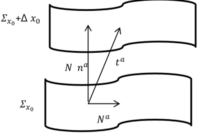
(2.10) The time-evolution vector or the deformation vector defined as the flow of time through space time is then decomposed into space and time components

(2.11) Where is called the lapse function and is defined as the rate of flow of proper time with respect to coordinate time as one moves along

2 THE HAMILTONIAN FORMALISM OF GR

26 is the shift vector and it measures how much the local spatial coordinate system shifts tangential to when moving from a hypersurface to another along [51].

Figure 2.1: we recall that the time-evolution vector as its name indicates, links two points of

the same coordinates of two neighboring slices which marks the evolution of time of this point.

From Eq. (2.11) we can write

_(2.13)

So the geometry of the space -time can be described by _{rather than}

2.3 The Hamiltonian formulation of a GR

Now, in aim to proceed with the Hamiltonian formulation of general relativity, we need first to rewrite the Lagrangian density in terms of the new variables _.

The Lagrangian density defined for vacuum space is given by

√ (2.14) where and is the scalar curvature.

𝑁𝑎

𝑁 𝑛𝑎 𝑡𝑎

𝛴𝑥

CHAPTER TWO. LOOP QUANTUM COSMOLOGY

27 As the space-time is foliated into hyeprsurfaces crossed by a flow of time-like curves, we need to determine a new scalar curvature defined on the 3 dimensional hypersurfaces. This is possible by defining a 3 dimensional Riemannian tensor in the same way we define a 4 dimensional Riemannian tensor through covariant derivatives

̃ (2.15)

Where ̃ is called the 3 dimensional intrinsic curvature tensor in terms of 4 dimensional

indices, is the 3 dimensional covariant derivative in terms of 4-dim indices on and a spatial 1-form. By using contractions with _{, we can find the intrinsic Ricci tensor and the}

intrinsic scalar curvature ̃. The intrinsic term is used to indicate that the variable describing the geometry of doesn‟t depend on the embedding of in .

Another important variable called the extrinsic curvature defined by

(2.16)

which describes the curvature of the hypersurface as seen by the 4 dimensional manifold, this means that it measures how the normal vector field changes with the way neighboring hypersurfaces are bending that‟s why it is an extrinsic feature of the geometry of [51,52]. Another way to define is

(2.17)

in which is the Lie derivative of with respect to the normal vector . One can see that

both (2.16) and (2.17) are equivalent weather you choose to see it as a change of with respect to the embedding of hypersurfaces or the change of the geometry of the hypersurface with respect to a parallel transport along the normal vector .

In aim to write the 4 dimensional scalar curvature in terms of the new variables

we write it first in terms of ̃ . Developing the Eq. (2.15) and using the projectors (from 3 dimensional variables written in 4 dimensional indices to the 4 dimensional space-time manifold indices ) we find the Gauss equation

̃ (2.18)

2 THE HAMILTONIAN FORMALISM OF GR

28 In the same way, using the definition of the 4-dim Riemannian tensor we find the Codazzi equation

(2.19)

The Ricci equation is expressed as

(2.20)

where is the space-time covariant derivative.

Using Eqs. (2.18), (2.19) and (2.20) the Gauss-Codazzi equation is given by

̃ (2.21)

Where is the ADM boundary term defined by

(2.22) in which is the normal acceleration.

The boundary term vanishes for because we assume a sufficiently large surface so the

boundary effects are negligible and the final Lagrangian density in ADM formulation is given by

√ ̃ (2.23)

where √ √ is easily found when we write the line element of space-time in terms of _as

( )( ) (2.24) Equation (2.23) can be written as

√

̃

(2.25)

The first thing to notice is that this Lagrangian density is free from terms with time derivatives of , which means that the canonical momentum of those variables vanishes

CHAPTER TWO. LOOP QUANTUM COSMOLOGY 29 { ̇ _̇ (2.26) Those two equations are the primary constraints of the system.

The canonical momentum of _{using Eq. (2.25) is given by}

̇ √ (2.27)

Now we can define the Hamiltonian density of the system as _̇

(2.28)

Where , are Lagrange multipliers and , .

From Eqs. (2.25), (2.27) and (2.28) the Hamiltonian density can be written as

(2.29)

Where is the Hamiltonian constraint given by

_√ ( ) √ ̃ (2.30)

And is the spatial Diffeomorphism constraint given by

(2.31)

From the primary constraints given by (2.26) we can deduce { ̇ { }

̇ { } (2.32)

and are called secondary constraints and are just Lagrange multipliers,

those constraints are first class constraints so they generate gauge transformations that don‟t change the physical information.

2 THE HAMILTONIAN FORMALISM OF GR

30 *Diffeomorphism constraint: let‟s suppose that the time-evolution vector is tangential to ( ), this can be interpreted as a tangent translation of to itself through a spatial diffeomorpic mapping.

*Hamiltonian constraint: in case where time-evolution vector has only a normal component ( ), this can be interpreted as a translation of forwards in the normal direction.

Hence, to generate time-evolution with the Hamiltonian density we need to specify both and . In aim to do this we first can notice that the constrained surfaces represent the physical space in which the Hamiltonian density vanishes, in another word there is no time-evolution with respect to an absolute time which is in agreement with general relativity. This implies that the evolution of the system can be seen as a gauge flow that is arbitrarily

CHAPTER TWO. LOOP QUANTUM COSMOLOGY

31

3 The Platini formulation of GR

3.1 The tetrad formalism

The basis vectors of a coordinate basis in the tangential space-time are written as

(2.33) Generally speaking, these basis vectors are not orthonormal.

Instead, orthonormal basis are of great interest in physics because working in such basis vectors means working in the local frame of the observer. The attempt to rewrite the theory of general relativity in terms of a new orthonormal coordinate basis called non-holonomic basis leads to the Platini action.

The non-holonomic basis vectors ̃ are defined by the inner product

̃ ̃ (2.34) where is the Minkowski metric and are called 4-dim internal indices.

We have ̃ then

̃ ̃ (2.35)

and equivalently for ̃ we have

̃ ̃ (2.36)

Both ̃ and are called tetrads, they hold all the information contained in and hence can

describe the geometry of the space-time instead of the metric . It is important to state that

under Lorentz transformations of the tetrad, the metric doesn‟t change, this gauge freedom is called internal gauge.

In aim to reformulate the Largrangian density given by Eq. (2.14) using the tetrad formalism we need to define first the covariant derivative in such a frame, which is given by

3 THE PLATINI FORMULATION OF GR

32 in which is a vector field in the orthonormal frame and is the connection 1-form given by

(2.38)

This can be seen as a parallel transport of the tetrad through the space-time manifold. In aim to preserve under the covariance derivation ( is everywhere the same when a

parallel transport is conducted via 1-forms connections), connection 1-forms have to be anti-symmetric on their internal indices

(2.39)

This requirement implies that the metric is also preserved and the connection 1-form is called Lorentz connection.

Now, we need to define the internal Riemannian tensor

(2.40)

Where is the space-time Riemannian tensor defined on the tangent space, it is given by

the covariant derivative as

(2.41)

By contractions we can find both internal Ricci tensor and the internal scalar curvature. The curvature of the connection is defined by

[ ] (2.42)

The imitation Riemannian on the tangent space then is given by

(2.43)

By contractions we can find both the imitation Ricci tensor and the imitation scalar curvature, so the Platini action reads

[ ] ∫ | | (2.44) This formalism is called “first order formalism”, where is the determinant of the tetrad .

CHAPTER TWO. LOOP QUANTUM COSMOLOGY

33 When differentiating the action with respect to the tetrad we find Einstein equations in the vacuum with the imitation Ricci tensor and the imitation curvature scalar. However, when differentiating with respect to the connection we find the compatibility equation that shows the covariance of the tetrad with respect to a covariant derivative defined by the connection . The constraints of this action are not closed under the Poisson brackets which may

complicates the quantization of the theory, a solution for this problem is to modify the Platini action to

[ ] ∫ | | _(2.45)

this modified action is called Holst-Platini action, where [ ] with the Levi-Cevita tensor and as the Immirzi-Barbero parameter.

3.2 The ADM formalism on the tetrad

As we did previously we split the tetrad into spatial and normal components then with a gauge fixing we define the normal component as the time component.

We define the spatial component as

(2.46) Where is the unit normal vector to the spatial surface and the normal internal vector to the internal spatial surface with .

Now, we need to fix the time component which is called the time gauge, we define the as the unit internal time-like vector and then . This means that we are working in the local frame of an Eulerian observer. We should mention that this gauge fixing doesn‟t affect the symmetry of the theory.

3.3 The Ashtekar’s variables

We define the spatial tensor called the densitized triad [53] by

3 THE PLATINI FORMULATION OF GR

34 Introducing this new variable to the Holst-Platini action and using Eqs. (2.45), (2.46) and (2.11) one can find after some calculations and integration by part that the variable canonically conjugate to called Ashtekar-Barbero connection is given by

(2.48) where is the spin connection defined through the covariant derivative in the tetrad

formalism over spatial vector fields, is related to the exterior derivative by

(2.49)

, are called Ashtekar‟s variables, their Poisson brackets are given by

{ } (2.50) { } { } (2.51) Now, we introduce the curvature of the

(2.52)

This is called also the strength field of .

The constraints in the tetrad formalism with the Ashtekra‟s variables of the Holst-platini action are then

{ √ ₍ ) (2.53)

The Gauss constraint generates gauge transformations as it implies gauge invariance in phase space. This is means that this constraint underlies a gauge symmetry under SU (2) group, which allows to adopt quantization methods used for Yang-Mills models.

It is also important to mention that Ashtekar connections (with complex Immirzi parameter) are simpler to manipulate then the real ones. For instance, the second term in the Hamiltonian constraint vanishes which simplifies the constraint. Ashtekar connections are associated to

CHAPTER TWO. LOOP QUANTUM COSMOLOGY

35 associated with a group of transformations that is not a subgroup of the Lorentz group which means that working with real connections under diffeomorphism is a difficult task. However, in loop quantum gravity it is much easier to quantize real connections then complex ones especially from Eq. (2.47), which means that the geometry is determined by and as a consequence the immirzi parameter needs to be real. Another problem arise from the fact that LQG works only with compact groups which is not the case for complexified SU(2) groups and it is much more complicated to find reality conditions for a quantized theory in a complex phase space [53].

4 ISOTROPIC LOOP QUANTUM COSMOLOGY

36

4 Isotropic loop quantum cosmology

4.1 Why holonomies?

Wilson loops were first introduced in the study of the strong confinement between quarks, they can be used to describe quantum states with quarks at ending points where they represent lines of non-Abelian electric fluxes and they turn out to be Eigen states of the Hamiltonian in the strong coupling limit.

The canonical quantization of gravity can induce some anomalies when writing the canonical commutation relations of the canonically conjugate variables of the phase space, for instance , where we expect a commutation relation of the form

[ ̂ ̂] (2.54) where ̂ is seen as the generator of q-translation. However, the scalar product in the Hilbert space is not invariant under those translations; this implies that the commutation relations need to be replaced. As a consequence, another approach was proposed by Rovelli and Smolin based on the quantization of the holonomy-flux algebra.

To introduce the definition of the holonomy, we need first to remind that Ashtekar

connections are elements of SU(2) group and the parallel transport of those connections along a curve is called holonomy

∫ (2.55) Where is the path operator, are the generators of the algebra of SU(2) groups and

are Pauli matrices [52].

4.2 Holonomy-flux algebra

The hypersurface is divided into faces delimited by edges , the idea introduced by Rovelli and Smolin is to use the holonomies along all the possible edges e of the hypersurface

, and fluxes on all the possible faces of the hypersurface as the new variables of the phase-space. Holonomies are already defined in (2.55), fluxes can be defined in the same way by smearing in two dimensions: given a 2-dim surface , is defined as

CHAPTER TWO. LOOP QUANTUM COSMOLOGY

37 ∫ (2.56) being and coordinates on the surface and the normal vector.

The Poisson brackets between holonomies and fluxes are

[ ] (2.57) [ ] (2.58)

Where is the sign of the scalar product .

4.3 The modified Friedman equation

As the universe is not static, the geometry of the spatial hypersurface can be described by the metric

(2.59)

where is the spatial metric independent of time and is the scale factor.

Now, we write the triad associated to the metric as

(2.60) where is the triad associated to the metric .

The next step will be to write Friedmann equations in terms of the real connections and their densitized triads. First, from Eq. (2.60) the densitized triad [50] can be written as

√

(2.61)

Where | | . Similarly, we find the connection

(2.62) Where ̇ and the dot denotes the derivative with respect to the cosmic time.

We can notice that the new variables and are canonically conjugate and can be taken as the new coordinates of the phase-space.

4 ISOTROPIC LOOP QUANTUM COSMOLOGY

38 Their Poisson brackets are given by

{ } (2.63) Where is the coordinate volume of the spatial hypersurface defined as

∫ (2.64) Now, we rewrite the Hamiltonian density in terms of the new variables. We find that both diffeomorphism and Gauss constraints vanishe because they are both solved by Eqs. (2.61) and (2.62) and we are left with the Hamiltonian constraint. The total Hamiltonian density including matter is then reduced to

∫ _(2.65)

Where is the Hamiltonian density for matter defined by

∫ ⁄ (2.66)

in which is the energy density.

The total Hamiltonian density then reads ⁄

⁄ _(2.67)

As the physical space is constrained by a vanishing Hamiltonian density we find that _(2.68)

and when squaring the Hubble parameter, it gives

̇ (2.69)

which is the Friedmann equation. This is expected since we are still working in the classical limit. Now, to introduce loop quantum corrections we need to work with holonomies and fluxes.

CHAPTER TWO. LOOP QUANTUM COSMOLOGY

39 Substituting Eq. (2.62) in Eq. (2.55) we find

| | _{( | | ) ( | | ) (2.70)}

where is the holonomy along a curve in the coordinate direction . The simplest loop (the holonomy along a closed graph) can be constructed from a square as

(2.71) Using Eq. (2.55) and the fact that the coordinate lengths of the sides of the square are equal we can write

( | | ) | | ( ) ( | | ) ( | | ) (2.72) The strength field of the connection is defined on a closed loop as

| |

* +

| | (2.73)

From Eq. (2.72) we find

| | | | _{| |} (2.74)

As the area operator has a non-vanishing minimum value in LQG, the coordinate length | | has also a minimum value | | so we can write

| _| |

| (2.75) The new modified Hamiltonian is given by

⁄

| |

| |

⁄ _(2.76)

The minimum coordinate length needs to be replaced by a fixed physical length

4 ISOTROPIC LOOP QUANTUM COSMOLOGY

40 This is due to the fact that the coordinate length depends on the coordinate choice which makes our Hamiltonian dependent on the coordinate choice. is usually defined as the square root of the minimum area gap of LQG [54].

As the Hamiltonian vanishes we find (

√ )

_(2.78)

To find the modified Friedmann equation we need to calculate the Hubble parameter, that is ̇ ̇ (2.79)

Then, we use the Hamiltonian equations of motion to get ̇ { } (

√ ) (√ ) (2.80)

Now, we replace this result in Eq. (2.79) and square (

√ ) (√ ) (2.81)

Using Eq. (2.78) we find the modified Friedmann equation expressed as

(2.82)

In which

41

Chapter three:

Modeling Dark Energy

By VMCG

“Not only is the universe

stranger than we think,

It is stranger than we can think”

Werner Heisenberg

CHAPTER THREE. MODELING DARK ENERGY BY VMCG

42

1

Viscous Modified Chaplygin Gas Model

1.1 Chaplygin Gas Models

In 1904, S. Chaplygin proposed, in the context of an aerodynamic research [55], a gas model with the equation of state

(3.1) where a positive constant, this model is also obtainable from Nambu-Goto action for d-branes moving in a (d+2) dimensional space-time. This fluid has the property of the only known fluid to admit a supersymmetric generalization.

From the conservation equation (1.21) of a universe filled with Chaplygin gas we find

√ (3.2)

where is an integration constant chosen to be positive and is the scale factor. At early times , we have a matter like behavior with

√ _(3.3)

At large scale and , we have a mixture of cosmological constant and stiff matter ( like behavior with

√ _{√ √ (3.4)}

At late time and we have a cosmological constant like behavior with

√ √ (3.5) The Chaplygin gas model behavior evolves in time from matter like behavior to a mixture of cosmological constant and stiff matter like behavior to finally a cosmological constant like behavior [13].

1 VISCOUS MODIFIED CHAPLYGIN GAS MODEL

43 The generalized Chaplygin gas with equation of state

(3.6) in which is a constant, is obtainable from Born-Infeld action [15].

In a universe filled with generalized Chaplygin gas, the conservation equation (1.21) gives _(3.7) in which is an integration constant.

At early times , we have a matter like behavior with

_(3.8)

At large scale, we have a mixture of cosmological constant and perfect fluid like behavior with

(3.9) where _.

At late time, we have a cosmological constant like behavior with

_(3.10) The generalized Chaplygin gas model behavior evolves in time from matter like behavior to a mixture of cosmological constant and perfect fluid like behavior to finally a cosmological constant like behavior.

The modified Chaplygin gas with the equation of state is given by

(3.11) where is a constant..