HAL Id: tel-00584109
https://tel.archives-ouvertes.fr/tel-00584109
Submitted on 11 Apr 2011HAL is a multi-disciplinary open access archive for the deposit and dissemination of sci-entific research documents, whether they are pub-lished or not. The documents may come from teaching and research institutions in France or abroad, or from public or private research centers.
L’archive ouverte pluridisciplinaire HAL, est destinée au dépôt et à la diffusion de documents scientifiques de niveau recherche, publiés ou non, émanant des établissements d’enseignement et de recherche français ou étrangers, des laboratoires publics ou privés.
une approche projective
Andreas Ruf
To cite this version:
Andreas Ruf. Couplage mouvements articulées - vision stéréoscopique : une approche projective. Human-Computer Interaction [cs.HC]. Institut National Polytechnique de Grenoble - INPG, 2001. English. �tel-00584109�
THESE
pour obtenir le grade de DOCTEUR de l’INPGEcole Doctorale: Math´ematique, Science et Technologie de l’Information Sp´ecialit´e: Informatique (Imagerie, Vision et Robotique)
pr´esent´ee et soutenue publiquement le 15. f´evrier 2001 par
Andreas
R u fClosing the loop between articulated motion and
stereo vision: a projective approach
Th`ese pr´epar´ee au sein du laboratoire gravir–imag et inria Rhˆone-Alpes sous la direction de
Radu Horaud
Jury :
Pr´esident : Philippe C in q u in
Rapporteurs : Fran¸cois C h a u m e t t e
Gerald S o m m e r
Examinateurs : JamesC r o w le y
Olivier F a u g e r a s
Directeur de th`ese: Radu H o r a u d
RUF
CINQUIN
CHAUMETTE
SOMMER
CROWLEY
FAUGERAS
HORAUD
I’m very grateful to Radu Horaud for advising me during the time of this thesis. He indicated directions which turned out very fruitful, and generously offered the liberty and the time I needed to explore and to conclude.
I’d like to thank the reseachers in the MOVI project for their cordial re-ception and support. In particular, I’d like to thank in particular Gabriella, to whom I owe a quick start and many open discussions, Bill and Peter, who selflessly agreed to proof-read the manuscript during a very busy season, and Frederick, to whom I owe excellent experimental results thanks to his DEA project.
I’d like to thank the jury for their thorough work, and especially the reviewers Gerald Sommer and Francois Chaumette for the quick and careful reading, and thoughtful comments.
Finally, there are all the friends who accompagnied and carried me through the ups and downs of life during this period, und meine Familie, bei der ich mich daf¨ur entschuldige, dass wir uns zu selten sehen konnten.
R´esum´e Cette th`ese propose un nouvel ´eclairage sur le couplage de la vision st´er´eoscopique avec le mouvement articul´e. Elle d´eveloppe tout par-ticuli`erement de nouvelles solutions s’appuyant sur la g´eom´etrie projective. Ceci permet notamment l’utilisation des cam´eras non-calibr´ees.
La contribution de cette th`ese est d’abord une nouvelle formulation g´eo -m´etrique du probl`eme. Il en d´ecoule des solutions pratiques pour la mod´ eli-sation, l’´etalonnage, et la commande du syst`eme. Ces solutions suivent une approche “coordinate-free”, g´en´eralis´ees en une approche “calibration-free”. C’est `a dire, elles sont ind´ependantes du choix des rep`eres et de l’´etalonnage des cam´eras.
Sur le plan pratique, un tel syst`eme projectif peut fonctionner sans con-naissance a priori, et l’auto-´etalonnage projectif se fait de mani`ere automa-tique. Les mod`eles propos´es sont issues d’une unification projective de la g´eom´etrie du syst`eme plutˆot que d’une stratification m´etrique. Pour un as-servissement visuel, les mod`eles obtenus sont ´equivalents aux mod`eles clas-siques. D’autres questions pratiques ont ainsi pu ˆetre abord´ees d’une nouvelle mani`ere: la commande de trajectoires visibles et m´echaniquement realisables dans l’espace de travail entier.
Sur le plan th´eorique, un cadre math´ematique complet est introduit. Il donne ´a l’ensemble des objets impliqu´es dans un asservissement visuel une repr´esentation projective. Sont notamment etudi´es, l’action des joints roto¨ides et prismatiques, les mouvements rigides et articul´es, ainsi que la notion associ´ee de vitesse projective. Le calcul de ces repr´esentations est de plus explicit´e.
mots cl´es: asservissement visuel, st´er´eo non-calibr´ee, cin´ematique sp´ecialit´e: Informatique (Imag´erie, Vision, Robotique)
GRAVIR-IMAG INRIA Rhˆone-Alpes, movi
655, avenue de l’Europe 38330 Montbonnot St.-Martin
Abstract In this thesis, the object of study are robot-vision systems consisting of robot manipulators and stereo cameras. It investigates how to model, calibrate, and operate such systems, where operation refers especially to visual servoing of a tool with respect to an object to be manipulated.
The main contributions of this thesis are to introduce a novel, “projec-tive” geometrical formalization of these three problems, and to develop novel coordinate- and calibration-free solutions to them.
The impact in practice: the “projective” systems can operate with less priori knowledge. Only metrically unstratified but projectively unified pa-rameters are needed to “calibrate” a fully operational model of the system. This can be done automatically with a self-calibration method. As far as visual servoing is concerned, the projective models are equivalent to classical ones. Also, their particular properties allow new answers to open questions in visual servoing to be found, such as how to control trajectories that are at the same time visually and mechanically feasible over the entire work-space. The impact on theory: a novel and complete projective framework has been introduced, that allows calibration-free representations for all basic ge-ometrical objects relevant to visual servoing, or to camera-based perception-action cycles in general. Most important are the projective representations of rigid- and articulated motion, as well as the respective notion of projective velocities. Effective computational methods for the numerical treatment of these representations were also developed.
keywords: visual servoing, uncalibrated stereo, coordinate-free kine-matics
GRAVIR-IMAG INRIA Rhˆone-Alpes, movi
655, avenue de l’Europe 38330 Montbonnot St.-Martin
Zusammenfassung Die vorliegende Dissertation betrachtet Hand-Auge-Systeme bestehend aus einem Roboterarm und einer Stereokamera, mit dem Ziel einer sichtsystemgest¨utzten F¨uhrung und Regelung des Roboters. Die Fragestellung umfaßt dabei die Umsetzungschritte Modellierung, Kalibrie-rung und Betrieb eines solchen Systems, wobei die PositionieKalibrie-rung von Werk-zeugen bez¨uglich der zu manipulierenden Werkst¨ucke als Anwendungsbeispiel herangezogen wird.
Der wissenschaftliche Beitrag besteht in der Formulierung eines neuarti-gen Ansatzes zur mathematischen Beschreibung der Systemgeometrie, dessen formale Darstellungen nur auf Mittel der projektive Geometrie zur¨uckgreift. Dazu kommen durchg¨angig projektive L¨osungen f¨ur die drei Umsetzungss-chritte. Sie zeichnen sich insbesondere durch Unabh¨angigkeit sowohl von der Wahl des Koordinatensystems als auch von der Kamerakalibrierung aus.
Auswirkungen auf die Praxis k¨onnen entsprechend “projektive” Hand-Auge-Systeme haben, die auch ohne Vorgaben zur Systemkalibrierung in Be-trieb gehen k¨onnen. Hierzu wird die zuvor noch in metrische und projective Parameter aufgetrennte Kalibrierung durch eine vereinheitlichte projektive Parametrierung ersetzt, die automatisch mit einer Selbstkalibriermethode bestimmt wird. Beide Parametrierungen sind, zumindest zum Zwecke der bildbasierten Regelung, gleichwertig. Weiterhin ergab diese Parametrierung auch neue Antworten auf noch offene Fragestellungen, wie die Roboter-f¨uhrung entlang von wohldefinierten Trajektorien, die sowohl unter mech-anischen als auch unter visuellen Gesichtspunkten vom Hand-Auge-System realisierbar sind.
Auswirkungen auf die Theorie liegen in dem erstmals eingef¨uhrten pro-jektiven Formalismus zur kalibrierunabh¨angigen Darstellung, welcher alle grundlegenden Bestandteile von Hand-Auge-Systemen umfaßt und somit als vollst¨andig bezeichnet werden kann. Hervorzuheben sind hierbei die projek-tive Darstellung starrer und artikulierter Bewegungen sowie der entsprechen-den Geschwindigkeitsbegriffe. Der theoretische Beitrag wird noch aufge-wertet durch die Formulierung und Umsetzung der rechnerischen Methodik zur numerischen Behandlung der projektiven Darstellungen.
1 Introduction 16
1.1 Motivation . . . 16
1.2 Problem formulation . . . 19
1.3 Organization of the manuscript . . . 21
1.4 State-of-the-Art . . . 25
2 Fundamentals 30 2.1 Perspective camera and P2. . . 30
2.2 Stereo camera andP3 . . . 33
2.3 Displacements, rigid motion, and SE(3) . . . . 42
2.3.1 The Lie group SE(3) – displacement group . . . . 42
2.3.2 One-dimensional subgroups . . . 43
2.3.3 Projective displacements . . . 45
2.4 Velocity of rigid motion and se(3) . . . 47
2.4.1 Lie algebra se(3) . . . . 47
2.4.2 Velocity of rigid motion . . . 48
2.4.3 Projective representations of se(3) . . . . 50
2.5 Duality . . . 52
2.5.1 Duality inP2 . . . 53
2.5.2 Duality inP3 . . . 54
2.5.3 Duality of multi-columns and multi-rows in Pn . . . . 55
2.5.4 Duals of homographies . . . 56
2.6 Numerical estimation . . . 57
2.6.1 Projective reconstruction of points and lines . . . 57
2.6.2 Homographies between points, lines, and planes . . . . 58
3 Projective Translations 63 3.1 Projective representations . . . 63
3.1.1 Definition . . . 63
3.1.2 Jordan form . . . 64
3.1.3 Eigenspaces and geometric interpretation . . . 65
3.1.4 Generator . . . 67
3.1.5 Exponential and logarithm . . . 69
3.1.6 Lie group and Lie algebra . . . 69 3.2 Numerical estimation . . . 71 3.2.1 SVD-based method . . . 71 3.2.2 Algorithm . . . 72 3.2.3 Optimization-based method . . . 73 3.3 Experiments . . . 74 3.3.1 Gripper experiment . . . 75 3.3.2 Grid experiment . . . 75 3.3.3 House experiment . . . 76 4 Projective Rotations 78 4.1 Metric representations . . . 78 4.1.1 Orthogonal matrix . . . 78 4.1.2 Pure rotation . . . 79 4.2 Projective representations . . . 79 4.2.1 Definition . . . 79 4.2.2 Jordan form . . . 80
4.2.3 Eigenspaces and geometric interpretation . . . 81
4.2.4 Rodriguez equation and generator . . . 84
4.2.5 Exponential and logarithm . . . 86
4.3 Lie group and Lie algebra . . . 87
4.4 Numerical estimation . . . 88 4.4.1 Objective function . . . 89 4.4.2 Minimal parameterization . . . 89 4.4.3 Initialization . . . 90 4.5 Experiments . . . 90 4.5.1 Experimental setup . . . 91 4.5.2 Non-metric calibration . . . 91 4.5.3 Feed-forward prediction . . . 91 4.5.4 Homing . . . 92 5 Projective Kinematics 98 5.1 Kinematics of articulated mechanisms . . . 98
5.2 Projective Kinematics . . . 105
5.2.1 Projective kinematics: zero-reference . . . 105
5.2.2 Projective kinematics: general reference . . . 107
5.3 Projective Jacobian . . . 109
5.3.1 Projective Jacobian: zero-reference . . . 110
5.3.2 Projective Jacobian: general reference . . . 111
5.4 Numerical estimation . . . 113
5.4.1 Objective function . . . 113
5.4.2 Projective parameterization . . . 115
5.4.3 Metric parameterization . . . 117
5.5 Experiments . . . 118
5.5.1 Evaluation of image error . . . 119
5.5.2 Evaluation of metric error . . . 120
6 Projective Inverse Kinematics 122 6.1 Prismatic joints . . . 122
6.2 Single revolute joint . . . 124
6.3 Two revolute joints: general configuration . . . 125
6.4 Two revolute joints: parallel configuration . . . 127
6.5 Three revolute joints: arm configuration . . . 129
6.6 Three revolute joints: wrist configuration . . . 130
6.7 Six axis manipulator: PUMA geometry . . . 131
6.8 Numerical estimation . . . 131
7 Projective Trajectories 132 7.1 Cartesian trajectories . . . 132
7.2 Trajectories from a projective displacement . . . 133
7.2.1 Decomposition . . . 133
7.2.2 Generation of Cartesian motions . . . 135
7.2.3 Translation-first and translation-last motions . . . 138
7.3 Trajectories of primitive motions from mobility constraints . 139 7.3.1 Translation along an axis . . . 139
7.3.2 Revolution around an axis . . . 140
7.3.3 Revolution around a point in a plane . . . 140
7.4 Trajectories based on three points . . . 142
7.4.1 Decomposition . . . 144
7.4.2 Visibility . . . 146
7.4.3 Generation of Cartesian trajectories . . . 147
8 Projective Visual Control 149 8.1 Perception domain . . . 150
8.1.1 Single camera . . . 150
8.1.2 Stereo camera pair . . . 151
8.1.3 3D triangulation device . . . 152
8.2 Action domain . . . 153
8.2.1 Kinematic screws . . . 153
8.2.2 Projective screws . . . 157
8.2.3 Joint-space and joint-screws . . . 158
8.3 Projective control in an image plane . . . 159
8.4 Projective control in stereo images . . . 161
8.5 Projective Cartesian control . . . 163
8.5.1 Projective control in (τ, θr, θp)-space . . . 163
8.5.2 Discussion . . . 165
8.6 Experiments I . . . 168
8.7 Experiments II . . . 171
9 Summary 177 9.1 Practice . . . 177
9.2 Theory . . . 179
9.3 Conclusion and Perspectives . . . 181
A Mathematics 183 A.1 Matrix exponential and logarithm . . . 183
A.2 Lie groups and Lie algebras . . . 184
A.3 Adjoint map . . . 185
A.4 Representation theory . . . 187
A.5 Jordan canonical form . . . 188
1.1 Hand-eye coordination . . . 17
1.2 Visual Servoing . . . 20
1.3 Projective modelling . . . 22
2.1 Euclidean camera frame . . . 30
2.2 Affine camera frame . . . 33
2.3 Stereo camera - Euclidean frame . . . 34
2.4 Infinity in P3 . . . 35
2.5 Stereo camera - Projective frame . . . 37
2.6 Epipolar geometry . . . 38
2.7 Stratification hierarchy . . . 39
2.8 Rigid-stereo assumption: scene-based . . . 41
2.9 Canonical velocity . . . 45 2.10 Projective displacement . . . 46 2.11 Spatial velocity . . . 49 2.12 Body-fixed velocity . . . 50 2.13 Orbit . . . 51 2.14 Image error . . . 54
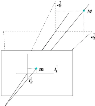
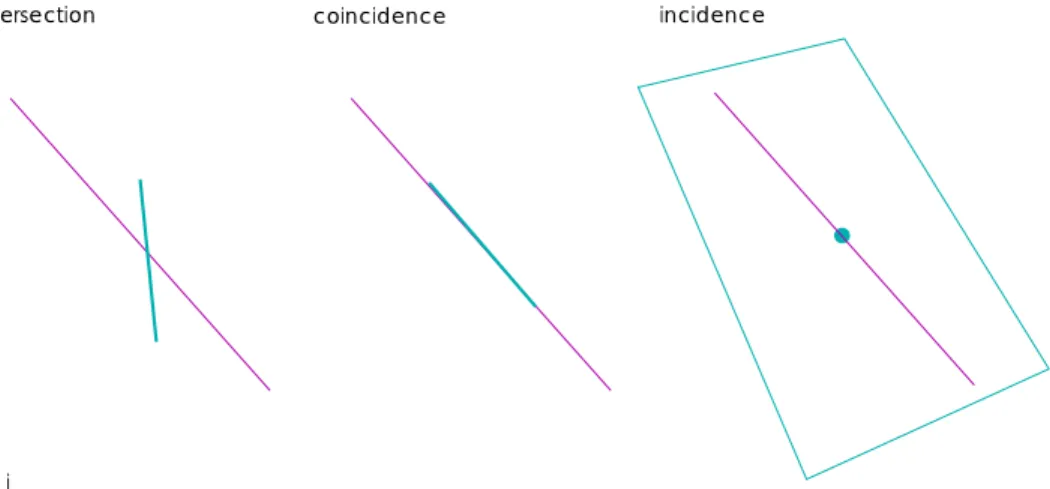
2.15 Intersection, Incidence, Coincidence . . . 59
2.16 Asymmetric constraints . . . 61 3.1 Jordan decomposition . . . 64 3.2 Eigenspaces . . . 66 3.3 Jordan frames . . . 68 3.4 Experiments: setup . . . 74 3.5 Results: noise . . . 75
3.6 Results: single vs. multiple translations . . . 76
3.7 Results: affine upgrade . . . 77
4.1 Jordan decomposition . . . 80
4.2 Geometric interpretation I . . . 83
4.3 Geometric interpretation II . . . 84
4.4 Velocity fields . . . 93
4.5 Experiments: Pan-tilt stereo camera . . . 94
4.6 Experiments: Pan-tilt mechanism . . . 94 4.7 Results: reprojection . . . 95 4.8 Results: image-error . . . 96 4.9 Results: prediction . . . 96 4.10 Results: homing . . . 97 5.1 Manipulator kinematics . . . 99
5.2 Forward kinematics: two frame . . . 100
5.3 Forward kinematics: workspace frames . . . 101
5.4 Forward kinematics: single frame . . . 101
5.5 Forward kinematics: camera frame . . . 102
5.6 Joint actions: camera frame . . . 103
5.7 Joint actions: tip-to-base order . . . 104
5.8 Projective kinematics: zero-reference . . . 106
5.9 Projective kinematics: camera frame . . . 107
5.10 Projective kinematics: inductive construction . . . 107
5.11 Projective kinematics: general form . . . 108
5.12 Projective Jacobian: general form . . . 112
5.13 Experiments: trial motions . . . 114
5.14 Experiments: image data points . . . 115
5.15 Experiments: image trajectory points . . . 119
5.16 Experiments: virtual rigid structure . . . 119
6.1 Prismatic Joints . . . 123
6.2 A revolut joint . . . 124
6.3 Two revolut joints . . . 126
6.4 Two revolute joints (parallel) . . . 127
6.5 Cosine theorem . . . 128
6.6 Arm configuration . . . 129
6.7 Wrist configuration . . . 130
7.1 Projective alignment . . . 133
7.2 Cartesian motion . . . 134
7.3 Decomposition rotation & translation . . . 135
7.4 Cartesian motion: two components. . . 136
7.5 Cartesian motion: instantaneous . . . 137
7.6 Grasp: rotation-first . . . 138
7.7 Constraints: translation along an axis . . . 140
7.8 Constraints: rotation around an axis . . . 141
7.9 Constraints: rotation in a plane . . . 142
7.10 Constraints: face with three points . . . 143
7.11 Visibility for translation . . . 143
7.12 Visibility for rotation . . . 144
8.1 Projective Control: Cartesian three components . . . 164
8.2 Projective Control: Cartesian two components . . . 168
8.3 Projective Control: image-based . . . 169
8.4 Experiments I: set-points . . . 170
8.5 Experiments I: transfer of set-points . . . 170
8.6 Experiments I: two tasks . . . 171
8.7 Results I: joint-space . . . 172
8.8 Results I: image-error . . . 172
8.9 Results I: simple task . . . 173
8.10 Results I: difficult task . . . 173
8.11 Results I: image-space . . . 173
8.12 Results I: joint-space . . . 173
8.13 Experiments II: benchmark . . . 174
8.14 Experiments II: failure . . . 174
8.15 Results II: visually feasible . . . 174
8.16 Results II: translation first . . . 174
8.17 Results II: direct3 vs ˙direct2 . . . 175
8.18 Results II: gains, limits . . . 175
8.19 Results II: control-error 2 . . . 175
8.20 Results II: control-error 3 . . . 175
8.21 Results II: image error . . . 176
8.22 Results II: joint-space . . . 176
9.1 Next generation visual servoing . . . 181
Journals
Andreas Ruf and Radu Horaud. Visual servoing of robot manipulators, Part I : Projective kinematics. International Journal on Robotics Research, 18(11):1101 – 1118, November 1999.
Conferences Tutorial
Andreas Ruf and Radu Horaud. Coordination of Perception and Action: the projective approach. European Conference on Computer Vision, Dublin, Ireland, June 2000.
http://www.inrialpes.fr/movi/people/Ruf/rufECCV00b.pdf Invitation
Andreas Ruf. Representation of Perception-Action Cycles in 3D projective frames. Algebraic Frames for the Perception-Action Cycle (AFPAC’00), Kiel, Germany, September 2000.
http://www.inrialpes.fr/movi/people/Ruf/rufAFPAC.pdf Papers
Andreas Ruf and Radu Horaud. Vision-based guidance and control of robots in projective space. In Vernon David, editor, Proceedings of the 6th European Conference on Computer Vision (ECCV’00), volume II of Lecture Notes in Computer Science, pages 50–83, Dublin, Ireland, June 2000. Springer. Andreas Ruf, Fr´ed´erick Martin, Bart Lamiroy, and Radu Horaud. Visual control using projective kinematics. In John J. Hollerbach and Daniel E. Koditscheck, editors, Proceeding of the International Symposium on Robotics Research, (ISRR’99), Lecture Notes in Computer Science, pages 97–104, Salt Lake City - UT, October 1999. Springer.
Andreas Ruf and Radu Horaud. Rigid and articulated motion seen with an uncalibrated stereo rig. In Tsotsos John, editor, Proceedings of the 7th International Conference on Computer Vision (ICCV’99), volume II, pages
789 – 796, Kerkyra, Greece, September 1999. IEEE Computer Society. Andreas Ruf and Radu Horaud. Projective rotations applied to non-metric pan-tilt head. In Proceedings of the Intl. Conf. on Computer Vision and Pattern Recognition, (CVPR’99), volume I, pages 144 – 150, Fort Collins, CO, June 1999. IEEE Computer Society.
Andreas Ruf, Gabriella Csurka, and Radu Horaud. Projective translations and affine stereo calibration. In Proceedings of the Intl. Conf. on Computer Vision and Pattern Recognition, (CVPR’98), pages 475 – 481, Santa Bar-bara, CA, June 1998. IEEE Computer Society.
Gabriela Csurka, David Demirdjian, Andreas Ruf, and Radu Horaud. Closed-form solutions for the Euclidean calibration of a stereo rig. In Burkhardt Hans and Neumann Bernd, editors, Proceedings of the 5th European Confer-ence on Computer Vision, (ECCV’98), volume 1, pages 426 – 442, Freiburg, Germany, June 1998. Springer Verlag.
Workshops
Ruf Andreas. Visual Trajectories from Uncalibrated Images. at Intl. Conf. on Intelligent Robots and Systems, (IROS 1997), In Proc. of Workshop on New Trends in Image-based Robot Servoing, pages 83 – 91, Grenoble, France, September 1997. INRIA.
Ruf Andreas. Non-metric geometry of robotic manipulation. at European Conference on Computer Vision, (ECCV 1998), Workshop on Visually guided robots: Current research issues and industrial needs Freiburg, Ger-many, June 1998.
Introduction
1.1
Motivation
The human capacity to control movements based on visual perceptions is called hand-eye coordination. By analogy, a technical system build from video cameras, robotic actuators, and computing devices should also be ca-pable of hand-eye control. A technology called “visual servoing” implements such “perception-action-cycles” as a closed-loop robot control, where feed-back and set-points are video-images captured on-line.
Human hand-eye coordination nicely exemplifies the various charac-teristics and potentials of this paradigm. From primitive tasks like reaching and grasping, through still simple tasks like tracking, pointing, and shoot-ing, to skilled craftsmanship and precision manufacturshoot-ing, the various com-plexities of hand-eye skills remind of an evolution from gatherer, through hunter or warrior, to craftsmen. The latter are a good example how hu-mans acquire skills very efficiently from learning-by-doing or, more precisely, from learning-by-seeing. For example, photos, sketches, or exploded-views in assembly instructions for take-away furniture or construction-toys (Fig. 1.1) can be seen as high-level “programs” for sequences of hand-eye skills, that almost anybody can follow. Finally, standardized engineering-drawings, CAD/CAM file formats, and in particular the connection of CNC machining with vision-based quality-control marks the transition from human towards technical hand-eye-coordination.
Technical hand-eye-coordination should ideally be as flexible, effec-tive, and intelligent as its human counterpart, while retaining the speed, efficiency, and power of machines. These dual goals mean that hand-eye-coordination is at the crossroads between artificial intelligence and machine vision in computer science, robot- and video-technology in engineering sci-ence, and fundamental control theory, mechanics, and geometry in applied mathematics. In very general terms, the overall aim is to produce a desired 3D motion of the manipulator by observing its position and motion in the
Figure 1.1: A hand-eye sketch from an assembly manual for a do-it-yourself lamp (left), and an exploded-view describing a construction-toy (right).
images, and using these observations to calculate suitable controls for the actuators. For expressing the interaction between perceptions and actions, it is therefore necessary to model the geometry of the system, and to calibrate it.
From a merely scientific point-of-view, Euclidean geometry provides ready-to-use concepts like rigid motion, kinematics, and linear camera op-tics, which make the geometric modeling of the robot-camera system straight-forward. However, “calibration” – identifying all parameters such a visual servoing system under real-world conditions – remains a difficult and time-consuming problem, both, technically and methodologically.
Distances measured in a Euclidean ambient space allow for the control-error to be defined in workspace, for it to be visually measured, and for a corresponding workspace-based control-law to be derived. Whenever such a control-loop servos the robot actuators to drive the distance-error to zero, it is ensured that the hand-eye-coordinated action or motion has achieved to desired target. Think of an assembly task specified for instance in terms of a drawing, e.g. of take-away furniture. It would be considered completed as soon as the video-image shows the various parts to have the desired
align-ment. Here, all the visual servoing loop does is to control the robot towards a position at which the video image captured by the on-line camera is in perfect alignment with the default image on the drawing. Obviously, this re-quires the on-line camera to be calibrated with respect to the drawing. This is related to the problem of camera calibration, for which various approaches already exist.
Off-the-shelf calibration uses manufacturer data, calibration devices, and on-site manual measurements to identify and estimate the model pa-rameters. Although the results obtained often lack stability and accuracy, and in some cases only a coarse guess is possible, the robustness inherent in the hand-eye approach ensures that the control still converges in most cases. However, systems that require accurate high-speed tracking of complex tra-jectories for global operability across the whole 3D-workspace, usually are only feasible if the quality of calibration is better than coarse.
More recent calibration techniques, especially for self-calibration of video cameras, use recent results in “uncalibrated” computer vision to idtify camera parameters without prior knowledge of either the present en-vironment, or the factory-given parts of the system. Although these tech-niques are rapidly becoming mature, they apply only to the “eye”, while the “hand”, the arm, and in particular the hand-eye relation still require an external calibration in form of a sophisticated procedure, called “hand-eye-calibration”. Moreover, a prior kinematic model of the robot is still required, e.g. from the manufacturer, deviations from which greatly influ-ence the overall coherency and accuracy of the system and its calibration.
Coordinate-free methods seek formal representations, distance met-rics, and computational algorithms that are independent of ad-hoc choices of coordinate-systems. Geometrically, the latter often refer to a profusion of frames associated with the various components to be modeled. For instance, a classical model would allocate frames on robot-base and -hand, on each linkage, on the tool, and on the camera. The hand-eye link or Denavit-Hartenberg parameters of each linkage are examples of representations that fail to be coordinate-free. A coordinate-free representation, in contrast, would be based on joints rather than linkages, and would represent them by their respective group actions on the ambient three-space. Such representa-tions often have fewer singularities, and greater generality, giving a theory that is both more powerful and more flexible, revealing the inherent nature of the underlying problem.
From an abstract scientific point of view, projective geometry de-scribes the geometric space of optical rays through a center of projection, and provides the mathematical concepts for perspective projection, geometrical infinity, coordinate-systems based on cross-ratios, and respective perspective transformations. Recent research in computer vision has successfully used these tools to model “uncalibrated” cameras, and to coherently describe the geometry of multiple uncalibrated cameras. In this context, “uncalibrated”
means “calibration-free”, i.e. the metric parameters describing the camera lens, the physical dimensions of the CCD, and their relation with the frame grabber output are entirely unknown. These metric parameters are replaced by projective ones, such as the linear product with a projection matrices. For instance, the epipolar geometry of an uncalibrated camera pair can be encoded as a pair of projective matrices, which in turn allow stereo triangu-lation of the environment in a three-dimensional projective space.
Image-based methods are a class of techniques, for which projective calculations are particularly well-suited.
For instance, two images of a scene are equivalent to a 3D projective reconstruction. Images taken from different view-points, using possible dif-ferent lenses or cameras, or difdif-ferent acquisition systems, can be related to the original one by a projective transformation. As everything can so be expressed in terms of images coordinates, the metric information does some-how “cancel out”. In this sense, the metric calibration and the displacement of the cameras become transparent, i.e. they no longer appear explicitly in the equations.
For example, as soon as a pair of images depicts an object-tool align-ment, it corresponds to a calibration-free representation of the underlying assembly task, which is already well-suited for a visual servoing to be ap-plied.
Calibration- and coordinate-free methods are analogous in the sense that they aim produce algebraic frames suitable for representing the geometry underlying the problem, and sometimes even geometric algebras naturally arising from it. In hand-eye-coordination, they are complementary, in the sense that coordinate-free representations of the action domain and calibration-free representations of the perception domain cover both aspects of hand-eye coordination. Moreover, the similarity of the two paradigms suggests that their fusion is worth investigating, in particular in the context of stereo-based hand-eye systems.
1.2
Problem formulation
The thesis seeks to give new solutions to the problem of hand-eye coordina-tion, with special emphasis on the visual servoing of a robotic cell consisting of a stereo camera and a manipulator arm (Fig. 1.3). One common applica-tion is grasping an object from camera observaapplica-tions of the work-space (Fig. 1.2). In contrast to existing approaches, the general case of “uncalibrated” cameras is considered, which necessitates the integration of projective ge-ometry with known techniques for visual servo control. The uncalibrated stereo rig spans a projective ambient space, whereas robot kinematics are commonly formulated in Euclidean space. One can ask whether a projective analogue to classical kinematics exists, and whether such an approach is
Figure 1.2: “Visual servoing” stands for hand-eye coordination in a closed control loop. Its set-point is a target image e.g. of a grasp, and its error-signal is usually the distance between current and target image.
computationally feasible. More generally, can the integration of calibration-free vision and coordinate-calibration-free mechanics bring about a unification of rep-resentations, as well ?
A detailed formulation of the problems investigated is as follows: • Given an uncalibrated stereo system capturing projective observations
of a dynamic scene, is a notion of “projective motion” well-defined, and how can it be represented, calculated, and accurately estimated? How can this be done for general rigid-object motions, for elementary robot-joint motions, and for general articulated motions? Given an articu-lated mechanism, is a notion of “projective kinematics” well-defined, how can it be represented, calculated, and accurately estimated – “pro-jective robot calibration” ? Can the forward and inverse kinematics be solved projectively, i.e. in terms of mappings between joint-space and projective-space motions? What are the infinitesimal analogues of this?
• Given a robot manipulator operating inside a projectively observed workspace, is a notion of “projective control-error” well-defined? How can a law for “projective servo control” be derived and calculated? Does it converge? How can this be done for set-points and features in a single image, in an image pair, and directly in projective space? Considering joint-velocity control, is a notion of “projective dynam-ics” well-defined1, how can projective velocities be represented,
calcu-1We will consider only first-order motion parameters, here. Acceleration and forces
lated, and applied? Velocities of rigid-object motion, of points, and also of planes? Based on a dynamic model of the interaction between space and image-space, can the forward dynamics, mapping joint-velocities onto image-space joint-velocities, and the inverse dynamics, map-ping the image-velocities required to annihilate the control-error onto the required joint-velocity command be solved projectively?
• Given an alignment task in a calibration-free representation, is a notion of “projective trajectory” well-defined, and how can it be represented, calculated, and adapted to the task? Given an alignment of all six degrees of freedom of a rigid body, is a notion of “projective Carte-sian motion” 2 well-defined, and how can it be represented, derived, and calculated? Based on the object’s projective displacement or al-ternatively on the projective dynamics of object points and -planes, how can the alignment be decomposed into projective translations and projective rotations, and can the robot motions that drive these ele-mentary motions be used to produce the desired Cartesian trajectory? Is the solution still image-based or can a “direct projective control” be done? Can the trajectory approach cope with restricted visibility, large rotations, and global validity in work-spaces?
1.3
Organization of the manuscript
The manuscript is organized in 7 core chapters, enclosed by an introduc-tory and a concluding chapter, followed by a number of appendices. Below, a chapter-by-chapter overview on contributions and impact is given. The organization of the chapters themselves follows the general guideline: alge-braic characterization, geometric interpretation, analytical and differential properties, computational and numerical methods, experimental validation and evaluation.
• Fundamentals: In this precursory chapter, the concepts fundamental to this thesis are recapitulated and restated using the terminology and formalisms adopted also in the succeeding chapters. Basically, these are the projective geometry of uncalibrated stereo vision, and respec-tive 3D-reconstruction in projecrespec-tive space. The rigid-stereo assump-tion is made, on which most results of this thesis are based. Equally important are the geometry and representations of the displacement group as well as its differential geometry and the velocities of rigid motion. The integration of these two concepts then allows the notion of projective motion to be defined as the homographic transformations arising from rigid motion observed in a projective space, i.e. captured
2Cartesian motions move a fixed point on the body along a straight line and rotate the
Figure 1.3: Modelling of a robotic work-cell using a stereo camera pair.
with a rigid stereo rig. Finally, the basic computational methodol-ogy for calculating reconstructions and homographies is given in great generality, allowing for instance also line and plane features to be con-sidered.
• Projective Translations: This chapter introduces the calibration-free representation for the projective translation group, and character-izes the properties of this Lie group and its Lie algebra. It provides efficient computational techniques for calibration, forward- and inverse kinematics of prismatic joints, as well as for affine stereo calibration, which range from algebraic closed-forms, linear methods, to numer-ical optimization. The methods have been validated and evaluated experimentally.
• Projective Rotations: This chapter introduces the coordinate- and calibration-free representation for the projective rotation group, and characterizes the properties of this Lie group and its Lie algebra. “Ro-tation” refers to an axis which may have an arbitrary position in space, e.g. the single joints of a six-axis industrial manipulator. Efficient com-putational techniques for calibration, forward- and inverse kinematics of revolute joints are provided, as well as for a pan-tilt actuated stereo rig. The methods range from algebraic closed-forms, linear methods, to numerical optimization. The basic method is validated and evalu-ated experimentally on a pan-tilt mechanism.
• Projective Kinematics: This chapter combines the results of the two preceding ones to introduce coordinate- and calibration-free rep-resentations for projective articulated motion, in form of a product-of-exponentials. This comprises projective representations for the static as well as dynamic kinematics of a robotic mechanism. The latter has the form of a Jacobian relating joint-velocities to velocities of pro-jective motion, or to image velocities. The chapter provides efficient computational techniques for stereo-based self-calibration of a robot manipulator, and for its forward kinematics as well as forward and inverse kinematics of the velocity model. The methods range from the sound analytic form of the Jacobian and forward kinematics, over a linear matrix representation of the joints-to-image Jacobian, to a large bundle-adjustment for the non-linear refinement of the calibration ac-curacy. Additionally, a stratification of the kinematics is investigated. The methods are validated and evaluated experimentally in a self-calibration experiment of a six-axis industrial manipulator.
• Projective Inverse Kinematics: This chapter relies on the devel-opments in the preceding chapters and details solutions to the inverse kinematic problem for standard industrial manipulators. The contri-bution is to solve this problem from a projective kinematic model, only, which is more difficult than in the metric case, since only angular but no distance measures are available. It is a projective solution which renounces stratifying the representations. The main interest is in find-ing a restricted initial solution for initializfind-ing a subsequent numerical refinement. Moreover, the modular geometric solution had a strong impact on the subsequent chapter, in particular on the algorithm for finding the elementary components of an alignment task.
• Projective Trajectories: Two approaches to generate the trajec-tories of Cartesian motions from projective data are developed. The first is based on a projective displacement and affine stratification to identify a translational component. The second is based on projective velocities, and on constraining the motion of a face on the object under consideration. The same trigonometric formulae as in the inverse pro-jective kinematics are arising. Cartesian trajectories are then created as a product-of-exponentials of projective translations and one or two concentric rotations. Additionally, the visibility of the face is taken into account. The methods are tested on simulated realistic data. • Projective Visual Control: Two distinct approaches to visual robot
control are developed. The first consists in image-based visual servo-ing based on a projective kinematic model. It is presented in great generality where the numerous varieties of this approach are shown as special cases of a coordinate-free formulation of the system. In
partic-ular, the equivalence of the hand-eye and independent-eye systems is shown. Similarly, a calibration-free formulation is possible, assuming nothing more than a rigid structure associated with the tool, while camera and robot configurations now may vary.
Besides the 2D-approaches, also a 3D approach can be considered, where a projective instead of a Euclidean space requires to revisit the definition of control-error in 3D-points.
Second, the results of the trajectory chapter have given rise to a di-rectly computed feed-forward for trajectory control of Cartesian mo-tion. The computations essentials correspond to those done in trajec-tory generation, while the remaining degrees-of-freedom are considered as a feedback error, which can be used to avoid singularities or con-strained visibility.
The basic results are validated on a real visual servoing system, and the advanced techniques are tested against simulated data.
Notations
For a complete reference on the notations employed throughout this thesis, please refer to appendix B. Here, only the basic typesetting conventions for equations shall be stated. Plain Roman type stands for scalars a, b, c, indices i, j, k, and coefficients h21, k12, where Greek letters denote angles α, θ and scale-factors γ, λ, µ. Bold type stands for matrices T, H, J, P, which sometimes are accentuated with ¯ , ˆ , ˇ . Bold italic stands for vectors
q, M, S, m, s, where in the context of point-vectors, uppercase denotes
3D-points while lowercase denotes 2D-points. Finally, calligraphic type is used for naming frames, e.g. E, A, P.
1.4
State-of-the-Art
The following synopsis on the state-of-the-art aims to situate this work with respect to the main approaches and the key-papers in the field. It more-over aims to relate it to previously published work which has inspired or influenced the research, and to distinguish it from approaches that show a certain degree of similarity. Since an innovation coming out of this thesis is a novel combination of robot control and manipulator kinematics with computer vision and projective geometry, the bodies of knowledge proper to both these fields have been of equal importance.
Concerning the research literature on visual robot control, please con-sult [42] and references there, or [9] in the quite representative collection [33], for an exhaustive overview on the research literature on visual robot control. Above that, the theoretical concepts underlying task- and sensor-based control are abstracted and formalized as the “task-function approach” introduced in the textbook [65]. Finally, two rather geometrical textbooks on robotics and kinematics, [66] and [57], have been a rich source of inspi-ration, and are quite close to the paradigms adopted in this thesis. More classical treatments are [5], [10], or the very didactic, but concise [55]. Ad-ditionally, the related problem of robot calibration is well covered by [56].
Concerning literature on computer vision or formerly “robot vision” [40], a number of excellent textbooks are already available for an in-depth and rather complete coverage of nowadays available solutions and computational methods: [37], [20], or [45] and more recently [29], which are very close to the scientific approach adopted in this thesis. In addition, a new collection of research work concerned with unifying the geometric approaches to robotic as well as vision problems is since recently available in [69].
One of the scientific pillars this thesis has been founded on is the notion of “projective motion”, more precisely “projective rigid motion”. It can be considered as a unifed formal and computational framework related to the classical problems in computer vision, such as pose, structure-from-motion (SFM), and binocular stereo vision. In this context, it is of interest what level of prior knowledge of camera calibration is required, since a fundamen-tal question addressed in this thesis is what degree of calibration is inherent to the visual robot control, and what requirements have been made in the past just for the sake of technical convenience.
Object pose [27] from a single image requires both, a metric model of the object and the camera’s intrinsic parameters in these metric units. This notion has given rise to the so-called position-based approach to visual ser-voing, see e.g. [80], for instance, or [75] which emphasizes more the pose-tracking problem. Structure from motion (SFM) [48] – more precisely struc-ture and motion from an image pair – requires the intrinsic parameters, only, and yields a metric model of the object and the camera’s motion in between the images, up-to a length scale, only. Visual servoing based on this has
been proposed in [73] for instance. A highly relevant special case is that of a planar object and its partial pose captured by the homography between two images of one and the same plane [6]. A respective visual servoing law has been introduced in [52], and extended to non-planar objects.
When internal camera calibration is no longer available, but only image correspondences, the essential matrix representing SFM becomes the funda-mental matrix representing the epipolar geometry of an image pair [49]. It is determined from at least eight points, and linear estimation is feasible and efficient [31]. Basic visual “homing” based on epipoles is actually proposed in [1]. Above that, the fundamental matrix allows for three-dimensional re-construction of scene-structure. In the uncalibrated case, [22], [30], it allows to recover structure and camera motion up to a fixed but unknown pro-jective transformation of the ambient space. Approaches to visual servoing which are trying to cope with such ambiguities are described in [25], [24], and [46]. A theoretical framework based on geometric algebras has been proposed in [2].
Reconstruction can be extended to a series of images, where respective factorization-based methods for multi-view reconstruction have successfully been applied , first to affine [74], and then to projective cameras [71]. Com-mon to most of these formulations is that the camera moving in or around a static scene is considered, and that it is camera motion which is recovered. In contrast, these methods cannot be applied immediately to a dynamic scene containing multiple objects moving relative to each other. Therefore, visual robot control, especially if an independently mounted camera is considered [39], is demanding rather for a sensorial system that yields a dynamic three-dimensional reconstruction of a dynamically changing environment. In the most general case, uncalibrated reconstruction is projective, and the respec-tive notion of three-dimensional dynamics in a projecrespec-tive ambient space is “projective motion”, as proposed in this thesis. In case of Euclidean three-space, discrete motion and pose is recapitulated in [82]. In the 2D projective case, the continuous motion seen by a single uncalibrated camera has been developed up to first-order in [77].
Projective motion output can be provided by stereo vision, which is con-sidered in combination with a computational method for triangulation as a proper device for triangulation, briefly called a “stereo camera”. The article [32] introduced such a method for triangulation, and discusses its properties when applied to ambient spaces of various geometries, from Euclidean to projective. Besides this polynomial solution in closed-form, a general itera-tive method, and also methods for reconstruction of lines have been proposed in [28] and [34], which are closely related to section 2.6.1, and a respective method for iteratively estimating projective motion [15], now from various features is developed in section 2.6.2.
A state-of-the-art application of projective motion is self-calibration of a rigid stereo rig [17], [83]. This can be done for the stereo camera undergoing
various types of rigid motion, among them ground-plane motions [11], [3] with respective degenerate situations [14]. The methods are closely related to the stratification hierarchy of geometric ambient spaces [21]. Among the special projective motions, pure translations and pure rotations with its axis in a general position – actually a general ground-plane motion is a non coordinate-free instance of a pure rotation – have so far been neglected. Fi-nally, they have been studied in-depth by the author [58], [59], where in par-ticular their potential for representing articulated motion and mechanisms has been exploited. Such motions, sometimes called “singular” motions, have been investigated with respect to degeneracies of self-calibration [72], and respective algorithms for partial or constrained estimation of epipolar geometries [78], camera calibration, or partial reconstructions [50].
However, those works are still using stratified representations, separat-ing camera calibration and Euclidean representations of motion, although equivalent projective representations, to which Euclidean and affine camera parameters are transparent, can indeed be defined, and have been introduced by the author [60]. Moreover, projective representations of articulated mo-tion and the kinematics of the underlying mechanism are equally possible, and respective calibration techniques have been demonstrated as feasible and accurate [62]. Above that, the notion of projective velocities of a point, a plane, or a rigid-body moving in a projective ambient space have been introduced in [61], (section 2.4.3) and [63]. In addition, the relationship between the chosen frame of the ambient space and the corresponding mo-tion representamo-tions has been revealed (see also A.3), which allows to show for instance that visual servoing of hand-eye and independent-eye systems is strictly equivalent from a theoretical point-of-view (section 8.2.1). Last but not least, the group property of projective displacements, i.e. of projec-tive rigid motion, its differential geometry as a Lie group, and its algebraic structure generated by the underlying Lie algebra have been identified [61]. Besides [18], few work has tried to explore the group-theoretical foundations of the visual servoing problem.
Most of the common approaches to visual servoing are neglecting the question of modeling or “kinematic calibration” of the robot actuator. Ei-ther an idealized Cartesian robot is considered [19], [51], or a six-axis in-dustrial manipulator is operated in the manufacturer’s Cartesian mode [26]. The effect of singularities [53], coupling [8], or inaccurate kinematics, also in the robot-camera linkage, are investigated rarely, and often no further than to the argument of asymptotic stability about the convergence of the closed loop.
Few approaches are controlling the robot-joints directly, and if, the cou-pling between the robot posture and the visual Jacobian is either covered by a coarse numerical approximation of a linear interaction model [44], which is valid only locally, or by an a-priori estimation of the interaction model, mostly locally around the goal and the robot’s configuration, there [70].
Convergence of such control laws has been observed, but little can be said about its performance in work-space, or about trajectories and convergence properties, there.
The same could be said about a “coarse calibration” of the camera and the hand-eye linkage, which generally means that factory given values for focal length, pixel size, and coarse, manual measurements of the hand-eye parameters are utilized. Again, the closed-loop will assure a narrow con-vergence for the visual goal to be reached, however, nothing can be said about performance with respect to the workspace goal, especially in case of an “endpoint-open” system (see [42]).
“Uncalibrated”, in first instance, refers to a visual task or goal which is formulated independent of the camera parameters. Clearly, projective invariance is the underlying concept, and [25], [24] tries to exploit such basic invariants for a number of simple alignment tasks. In [39] finally, a tool-to-object alignment in all 6 degrees-of-freedom is developed, based on a 5-point basis of projective space. This concept is also applied in [46]. The fact that “endpoint-closed” (see [42]) goals are considered implies the visual goal to be sufficient for a workspace-goal to be achieved.
Common to all these approaches is the “stratification” of projective cam-era parameters and projected visual motion against robot parameters or ar-ticulated motion. This stratification is most evident in [46], where the linear relationship between a projective frame for the work-space and a Euclidean frame for the robot is considered. However, the stratification of the model is vanishing as soon as it is contracted for instance to a robot-image Jacobian in matrix form [67], [68].
Therefore, the derivation of visual servoing laws based on projective kinematics representing the actuator, and on projective motion representing the demanded task and trajectory no longer requires a stratified model, unless for notational or technical convenience. It still results in respective interaction matrices, which are strictly equivalent and in which stratified parameters are transparent. Moreover, it allows for seamless integration with uncalibrated task-representations, including constrained trajectories, and projective calibration of robots.
Such an unstratified or “non-metric” visual servoing system obviously does change the calibration problem. Commonly, this problem has to be solved for the camera [23], the robot [79], and the camera-robot linkage [76]. The drawback of a stratified step-by-step calibration is that errors in the previous stage will affect the results of the succeeding steps, e.g. inaccurate kinematics rather quickly cause a hand-eye calibration to degenerate. Work already exists which tries to overcome this, [38], however rarely to an extent that calibration identifies also the kinematic parameters. Especially self-calibration techniques suffer from their generality and tend to instabilities due to the few and weak constraints available [72]. In contrast, the projec-tive self-calibration of a stereo-robot system, as proposed in this thesis, first
establishes an unstratified model for each robot joint, which yields already an operational and accurate system. Then, it combines them into a consis-tent, but still unstratified model of the kinematic robot-stereo interaction. Finally, if convenient, an a-posteriori stratification of the representations can be recovered, as well.
Fundamentals
2.1
Perspective camera and
P
2This section describes how the geometry of a perspective camera can be modeled algebraically in terms of projective plane and its transformation group, the latter allowing in addition the properties of the CCD video-sensor and the frame-grabbing device to be modeled.
raster plane image u v optical axis optical center pixel image object Y X Z E
Figure 2.1: Pinhole camera with Euclidean frame.
Euclidean camera frame
For representing a camera or a stereo camera pair, each camera is associated with a Euclidean frame, denoted E. It is allocated onto the camera in a
standard manner (Fig. 2.1). The optical center becomes the origin, the optical axis becomes the Z-axis, and the focal plane is taken as X-Y plane, where CCD-scanlines become the X-axis, but CCD-columns can be skew to the Y -axis. In such a frame, depth along the Z-axis is always orthogonal to the image-plane, hence to X- and Y -axis.
The frame E is spanning an ambient space which is Euclidean, and in which a Euclidean point has coordinates (X, Y, Z)>. It projects onto the image point (x, y)> µ x y ¶ = Ã f X Z f Y Z !
, with f the focal length.
Here, (x, y)> are coordinates in a plane, which has the principal point as origin, and the x- and y-axis aligned withE. Note, dividing by the depth Z makes this projection a non-linear one.
Homogeneous coordinates
Image coordinates can be formally extended to homogeneous ones by an ad-ditional third row (x, y, 1)>. This allows the 3-vector (X, Y, Z) to represent a point in E, and at the same time its image projection or equivalently the direction of its optical ray. In this context, the vector-space is divided into equivalence classes of non-zero 3-vectors with a free, unknown scale λ.
xy 1 = X Z Y Z 1 ' λ XY Z , with f = 1.
Thus, as soon as the length unit is set to f , homogeneous coordinates implicitly express the perspective projection of a pinhole camera (Fig. 2.1). Infinity
Usually, the representatives for such equivalence classes are chosen to be vectors with a 1 on the third row, since it is non-zero for all visible points. Additionally, the general or “projective” homogeneous coordinates allow op-tical rays to be represented that are actually “invisible”, i.e. that lie in the focal plane, and so have Z = 0. Formally, these are 3-vectors with a 0 on the third row. Geometrically, they form a “line at infinity” holding the “vanish-ing points” or the “directions” of the plane, where opposite directions, i.e. antipodal vanishing points are identified.
xy 0 = lim τ →∞ 1 τ τ xτ y 1 .
The set of non-zero homogeneous three-vectors are thus a representation of the projective planeP2. This geometric space is used in the sequel to model pinhole cameras and their image-planes.
Intrinsic camera geometry
In practice, there is still a transformation between the Euclidean image-plane (x, y, 1)>as a geometric entity, and the video-image (u, v, 1)>as a 2D-signal captured by the CCD and processed by the frame grabber. In (2.1), such a video-image is described in pixels of width 1/ku and height 1/kv, with skew kuv, where u0 and v0 are the pixel-coordinates of the principal point.
K = " kukuv u0 0 kv v0 0 0 1 # , (2.1) uv 1 = K xy 1 ' K XY Z . (2.2)
Please note, K is strictly speaking an affine transformation or an “affin-ity”, as the last row shows, whereas ' denotes projective equality up-to-scale.
Image transformations
The homogeneous coordinates in the projective plane P2 allow to represent projective transformations linearly in terms of the projective group P GL(2), whose elements are “homographies” or 2D-“projectivities”. They are repre-sented as 3× 3 homogeneous matrices H ∈ P GL(2) in such a context1. For example, the transformations of an image resulting from a camera rotating about its optical center are always such projectivities. In consequence, mis-alignments between the optical axis and the image-plane can so be modeled, e.g. a CCD failing to be exactly parallel to the focal plane.
uv 1 '= K R · XY Z . (2.3)
Still, algebraic QR-decomposition allows an arbitrary homography H to be rewritten in form of an upper triangular matrix K times an orthonormal matrix R, i.e. a rotation. Similarly, the later introduced three-dimensional projective space (2.7) will allow for a linear representation of perspective projection, although it is analytically a non-linear one.
U W V u optical v axis image plane raster image object optical center A pixel
Figure 2.2: Pinhole camera with affine frame. Affine camera frame
Based on K, an affine camera frameA, is well-defined, which can be thought of as being allocated onto the camera (Fig. 2.2). It spans an affine ambient space in which 3D-points are represented as (U, V, W )>, where U and V hold pixel-coordinates, and W holds depth-coordinates parallel to the optical axis in f units. It is indeed a general affine frame and no longer a Euclidean one, since the U - V -axes are skew, and since their scales differ, especially from the one on the W -axis.
uv 1 = U W V W 1 ' 1 0 00 1 0 0 0 1 UV W .
Note, in this particular frame, A, the camera parameters are trivially the identity I.
2.2
Stereo camera and
P
3Consider now a pair of pinhole cameras mounted onto a stereo rig, briefly called a “stereo camera” (Fig. 2.3). The basic properties of such a system are recapitulated in this section. It is presented as a triangulation device which
1The notationH is mainly used for space homographies, introduced later. Normally,
can be operated either in metric, in affine, or in projective mode, depending on the present degree of calibration. Such a device is used to recover a reconstruction of the three-dimensional workspace in the respective ambient space: Euclidean, affine, or projective camera-space, denotedE, A, or P.
This section concludes with the “rigid stereo assumption”, which most results of this thesis are based on. Briefly, it states that a stereo camera with a fixed geometry results in the transformations between the respective ambient spaces to be constant, as well.
E E’ camera space m m’ rigid object 3D point image plane left optical ray optical ray right image plane image point image point baseline rigid stereo rig X metric
Figure 2.3: Stereo camera with Euclidean frame.
Extrinsic geometry
Consider a pair of Euclidean frames,E and E0, on the left and right camera. Then, the extrinsic geometry of the rig is described by the pose of the right camera with respect to the left one. This is expressed as a rotation R followed by the translation t, which would move the right frame onto the left one, or analogously, which transforms the coordinates in the left ambient space to the right ones, indicated by a prime:
³X0 Y0 Z0 ´ = R ³X Y Z ´ +t.
The formal extension to a homogeneous fourth coordinate – see section 2.3 for a rigorous treatment – allows this transformation, which is non-linear in the summed form above, to be represented linearly as a single multiplication with a 4× 4 matrix: µX0 Y0 Z0 1 ¶ = · R t > 1 ¸ µX Y Z 1 ¶ = µ R µX Y Z ¶ +t 1 ¶ . (2.4)
Note, such matrices represent always a displacement, and thus represent the so-called “special Euclidean group” SE(3).
Infinity 8 τ 8 X( ) τ plane at infinity a8 T X( )
Figure 2.4: Plane at infinity in projective space P3.
In a Euclidean, and also in an affine context, a point homogenized to 1 is always a finite point, whereas points at infinity formally have a 0 on the forth row. Geometrically, they can be interpreted as vanishing points or “direc-tional” points of an endlessly2 continued translation along t = (X, Y, Z)> (Fig. 2.4). Since τ is unsigned, these directions are unoriented, and two antipodal vanishing points are thus coincident.
µX Y Z 0 ¶ = lim τ →∞ 1 τ µτ X τ Y τ Z 1 ¶ . (2.5)
Please note, this simple formal distinction between finite and infinite points is only valid in Euclidean or affine frames. A necessary condition on Eu-clidean and affine transformations is therefore that they leave this property invariant, which is indeed assured by the fourth row of a respective matrix equal (0, 0, 0, 1). µ∗ ∗ ∗ ρ ¶ = ·∗ ∗ ∗ ∗ ∗ ∗ ∗ ∗ ∗ ∗ ∗ ∗ 0 0 0 1 ¸ µ∗ ∗ ∗ ρ ¶ .
So,a>∞= (0, 0, 0, 1) necessarily are the Euclidean coordinates of the “plane at infinity” which contains all directional points.
Euclidean stereo camera
For the moment, let us continue with the classical modelling of a stereo camera, but let us use rigorously P3 and P2 to represent points in three-space and in the image-planes, respectively.
For a vector X holding homogeneous Euclidean coordinates in E, the left and right cameras can be written as in (2.7), where K0 are the right intrinsic parameters: m ' PE X, m0 ' P0E X, where (2.6) PE = " K ¯¯¯¯ 0 # , P0E = " K0R¯¯¯¯K0t # . (2.7)
Affine stereo camera
For a vector N holding homogeneous coordinates in A, the left projection matrix is the trivial one, and the right projection becomes respectively
m ' PA N, m0 ' P0A N, where (2.8) PA= " 1 0 0 0 0 1 0 0 0 0 1 0 # , P0A= " K0RK−1¯¯¯¯K0t # . (2.9)
Interestingly, for points at infinityN∞= (U, V, W, 0)>, the so-called infinity-homography H∞is well-defined, which maps their left imagesm∞onto right imagesm0∞:
H∞= K0RK−1, m0∞= H∞m∞.
Additionally, sincet relates to the left optical center in E0, the right epipole equalse0 =−K0t.
Projective stereo camera and epipolar geometry
Consider a number of 3D pointsM, and their matching left and right images
m and m0. Convince yourself that the two optical centers together with the
3D-point M form a plane which cuts the two image-planes in a line, each (Fig. 2.5). Its algebraic formulation is the epipolar constraint in form of a 3× 3 matrix, the so-called “fundamental matrix” F.
m>Fm0 = 0. (2.10)
It maps a right image point m0 to its corresponding epipolar line Fm0 in the left image, on which m must lie. It has been shown that at least 8 such point-correspondences determine the so-called epipolar geometry of the stereo camera (Fig. 2.5).
In the “uncalibrated” or “projective” case, the intrinsic parameters K, K0, and the extrinsic parameters R,t are supposed not to be known. In spite of that, a pair of projection matrices can be derived, which is consistent with
P in epipolar plane projection triangle metric rigid stereo rig camera space m m’ M rigid object 3D point image plane left optical ray optical ray right image plane epipolar line
line between opticals centers
projective camera space
image point image point
Figure 2.5: Stereo camera pair with epipolar geometry and projective frame. the present epipolar geometry. In [30], it is shown how a right projection matrix consistent with F can be defined,
m ' PP M, m0 ' P0P M, where (2.11) PP = h1 0 0 0 0 1 0 0 0 0 1 0 i , P0P = · [e0]F +e0a>¯¯¯¯e0 ¸ , (2.12)
and (a>, 1) is an arbitrarily fixed 4-vector. Triangulation
From a more abstract point-of-view, the above three projections (2.7),(2.9), (2.12) are three different models of one and the same stereo camera pair. They differ in the ambient space they are expressed in, Euclidean, affine, or projective. So, they differ in the camera frame a respective 3D-reconstruction refers to: E, A, or P. Geometrically, each of the equations (2.6), (2.8), or (2.11), describes a pair of optical rays (see section 2.6.1). Solving homoge-neous equations like the one in (2.13) for X, N, or M, amounts to inter-secting these rays, and yields a triangulation [32] of the respective ambient space relative to its proper coordinate frame.
projective: "£1 0-u 0 1-v ¤ · PP £1 0-u0 0 1-v0 ¤ · P0 P # ρM = . (2.13)
Figure 2.6: Stereo image-pair of a robot arm, matches, and their epipolar lines illustrating the pair’s epipolar geometry.
Homographies
Remember, the “projective three-space” P3 is the set of all finite and infi-nite points. They are represented by equivalence classes of non-zero, ho-mogeneous 4-vectors M = ρ (U, V, W, 1)> with a well-defined scale ρ. The corresponding transformation group are the spatial “homographies” or 3D-“projectivities”, always denoted as H ∈ P GL(3). This group is commonly written as 4× 4 homography matrices, which in general will alter a vector’s forth row M0= γ " h11h12h13h14 h21h22h23h24 h31h32h33h34 h41h42h43h44 # M.
It is worthwhile regarding how such homographies are well-defined. Since each point has 3 “degrees-of-freedom” (dof), and the homography matrix has 15 dof, 5 points in general position are necessary and sufficient for a matrix H to be well-defined, up to a scalar γ, however. So, five pairs of corresponding 4-vectors Ap and Bp, which actually amount to a pair of corresponding projective frames, allow the linear transformation between the two frames, A and B, to be calculated algebraically as follows [12].
λpAp = HBp, p = 1, . . . , 5 [B] = " B1 B2 B3 B4 # , [A] = " A1A2A3 A4 #
In the first instance, four points define an intermediate 4× 4 matrix H∗ re-lated to the solution by four scalars D = diag (λ1, λ2, λ3, λ4) on the columns.