Computation and approximation of the inverse of relationship matrices between genotyped animals: Algorithms and Applications

U

L

–

G

A

-B

T

C

OMPUTATION AND

APPROXIMATION OF THE

INVERSE OF RELATIONSHIP

MATRICES BETWEEN

GENOTYPED ANIMALS

:

A

LGORITHMS AND

A

PPLICATIONS

E

P

F

EN VUE DE L

’

P

:

N

G

U

L

–

G

A

-B

T

C

OMPUTATION AND

APPROXIMATION OF THE

INVERSE OF RELATIONSHIP

MATRICES BETWEEN

GENOTYPED ANIMALS

:

A

LGORITHMS AND

A

PPLICATIONS

E

P

F

EN VUE DE L

’

P

:

N

G

soit ou d'en autoriser la reproduction partielle ou complète de quelque manière et sous quelque forme que ce soit. Toute photocopie ou reproduction sous autre forme est donc faite en violation de la dite loi et de des modifications ultérieures.

English). Gembloux, Belgium, Gembloux Agro-Bio Tech - University of Liège, 139p., 21 tabl., 24 fig.

Abstract

The recent developments in molecular biology have made available thousands of genetic markers, allowing livestock genotyping at a reasonable cost and the subsequent development of genomic prediction. The single-step procedure, a unified approach of genomic prediction, requires inversion of two matrices gathering additive relationships between genotyped animals: the genomic relationship matrix (G) and a part of the additive relationship matrix (A22). The inverse of A22 may also be interesting for other

applications. Matrix inverse can be constructed successively by, first, computing, for each animal, the vector containing contributions of other animals to its relationship and, secondly, adding the product of each vector of contributions by itself to a zeroed matrix. The objectives of this thesis were (1) to propose algorithms to compute or to approximate the vector of contributions and (2) to test the numerical efficiency of these algorithms (computing speed, memory use and, if needed, approximation accuracy). Computing contributions covered two points: (1) finding or approximating which contributions are different from zero, and (2) computing the value of contributions considered as non-zero. In the first approach, we considered that animals closely related have non-zero contributions and approximated their values by linear regression. This approach was extended in a recursive way. In the second approach, we empirically determined the set of non-zero contributions by a heuristic algorithm of pedigree exploration (only for the case of A22). Values were then computed either by linear regression, or using the already

computed inverse. We also tested an approximation strategy: limiting the number of extracted generations of non-genotyped ancestors to reduce pedigree complexity. In a third approach, we followed the same heuristic algorithm as before but restricted the pedigree exploration to find out which animals have a non-zero contribution. Their values were approximated by linear regression. The presentation of the different approaches is followed by a general discussion in which the approaches are compared. It was found that the best compromise between speed, memory and approximation accuracy was achieved by the last approach for the case of A22. Use of this last approach simplified computations

and therefore made predictions more feasible. However, for the case of G, no sufficient approximations could be reach in a reasonable time. Perspectives of other uses of algorithms developed and of future researches were drawn, as well as practical perspectives for animal breeding.

Gembloux, Belgique, Gembloux Agro-Bio Tech - Université de Liège, 139p., 21 tabl., 24 fig.

Résumé

De récents développements en biologie moléculaire ont rendu disponibles des milliers de marqueurs génétiques, permettant de génotyper les animaux de rentes à un coût modéré et, conséquemment, le développement de la prédiction génomique. La procédure « single-step », une approche unifiée de prédiction génomique, requiert l’inversion de deux matrices rassemblant les parentés additives entre animaux génotypés : la matrice de parenté génomique (G) et une partie de la matrice de parenté additive (A22).

L’inverse de A22 peut également être intéressante pour d’autres applications. L’inverse

d’une matrice peut être construite successivement : premièrement, en calculant, pour chaque animal, le vecteur qui contient les contributions des autres animaux aux parentés de celui-ci et, deuxièmement, en ajoutant le produit de chaque vecteur de contributions par lui-même à une matrice nulle. Les objectifs de cette thèse sont (1) de proposer des algorithmes pour construire ou approximer le vecteur des contributions et (2) de tester l’efficience numérique de ces algorithmes (temps de calcul, usage de mémoire et, si nécessaire, précision de l’approximation). Calculer les contributions recouvre deux aspects : (1) trouver ou approximer quelles sont les contributions non-nulles, et (2) calculer les contributions considérées comme non-nulles. Dans la première approche, nous considérons que les animaux fortement apparentés ont des contributions non nulles et approximons leur valeur par régression linéaire. Cette approche est étendue dans une implémentation récursive. Dans la seconde approche, nous déterminons empiriquement l’ensemble de contributions non-nulles par un algorithme heuristique d’exploration du pedigree (seulement pour le cas de A22). Les valeurs sont alors calculés soit par régression

linéaire on en utilisant l’inverse déjà calculé à ce point. Nous testons aussi une stratégie d’approximation : limiter le nombre de générations extraites d’ancêtres non-génotypés pour réduire la complexité du pedigree. Dans une troisième approche, nous suivons le même algorithme heuristique qu’avant mais restreignons l’exploration du pedigree pour trouver quels animaux ont une contribution non-nulle. Leur valeur est approximée par régression linéaire. La présentation des différentes approches est suivie par une discussion générale dans laquelle les approches sont comparées. Il a été montré que le meilleur compromis entre consommation de temps et de mémoire et justesse de l’approximation était réalisé par la dernière approche dans le cas de A22. Utiliser cette dernière approche

simplifie les calculs et donc rend les prédictions plus faisables. Cependant, pour le cas de

G, aucune approximation suffisante n’a pu être atteinte en un temps raisonnable. Des

perspectives d’autres utilisations des algorithmes et de futures recherches sont esquissées, aussi bien que des perspectives pratiques pour l’amélioration animale.

« Spirou, viens voir la nouvelle idée de Fantasio pour le bal costumé... C’est original, mais si on danse?...»

In early 2009, I came in Gembloux and knocked on the door of Prof. Nicolas Gengler. My everlasting interest for animal breeding brought me there. I was looking for a short-time position in an animal science research group, where I could simultaneously work and learn the basic and advanced principles of genetic evaluation. But Nicolas had a much better plan than a short-time position: a PhD in collaboration with CONVIS s.c. and University of Georgia (UGA). This plan allowed me to be part of a wonderful research group, to enjoy the work with them and to learn not only about genetic evaluation but also – mostly, should I say – about numerical calculus, programming and maths. It allowed me as well to travel in Europe and to USA where I met many other great people. For initiating the PhD project and for pushing me ahead in its achievement, I would address to Nicolas, my supervisor, sincere and warm thanks.

This was also made possible thanks to the thesis committee that advised me every year and to the thesis jury that read and reviewed the thesis. Therefore, I would like to personally acknowledge each member of these committee and jury. The thesis committee members were Prof. André Théwis, Prof. Rodolphe Palm and Prof. Yves Beckers, all from Gembloux Agro-Bio Tech (GxABT), Mr. Jean Stoll (formerly CONVIS s.c.), Mr. Romain Reding (CONVIS s.c) and Mrs. Jeanne Bormann (Administration et Services Techniques de l’Agriculture du Luxembourg, ASTA). Mrs Jeanne Bormann is also part of the thesis jury, as well as Prof. Frédéric Francis (President of the thesis jury) and Prof. Catherine Charles, both members of GxABT, Prof. Frédéric Farnir (Faculty of Veterinary Medicine of the University of Liège) and Dr. Ignacy Misztal (University of Georgia). I would like to address special thanks to Mrs. Jeanne Bormann and Prof. Catherine Charles that read the first draft of my thesis. Thanks to their helpful comments, my initial document has been improved significantly.

My gratitude also goes to Dr. Ignacy Misztal. During my “American” time, Ignacy delivered me so many advices. Those were precious and precise, numerous and … numeric, obviously! But they went far beyond the strictly professional area. Thank you, Ignacy, for all these moment we have spent aside of the work, talking about numerous and various subjects while seating at a good table or sharing a good drink.

extend my gratitude to the following people for the fruitful discussions we had: Shogo Tsuruta (UGA), Selma Forni (Genus PIc, USA), Andrès Legarra (Institut National de la Recherche Agronomique, France), Ignacio Aguilar (Instituto Nacional de Investigacion Agropecuaria, Uruguay), Gregor Gorjanc (University of Ljubljana, Slovenia and Roslin Institute, Scotland) and Jérémie Vandenplas (GxABT).

I would also acknowledge the institutions that surrounded my project through a special thank to the following people: Mrs. Marie-Claude Marx and Mrs. Susana Pinto, from the Fonds National de la Recherche Luxembourg that funded the four first years of the PhD project; Mr. Romain Reding, Mr. Jeff Stirn and Mr. Armand Braun, from CONVIS s.c.; Mr. Alain Gillon from the Walloon Breeding Association (AWE). In addition, I would like to acknowledge the Ministry of Walloon Region for funding the remaining seven months of PhD.

My final thanks go to the research teams to which I have been part of: all members of the Animal Science Unit of Gembloux Agro-Bio Tech and of the Animal Breeding and Genetics Group of the Animal Dairy Science Department of the University of Georgia. Among those people, an additional thanks goes to: Valérie Arnould, with whom I have been closely working on Luxembourg data; Catherine Bastin, Frédéric Colinet and Jérémie Vandenplas, for revising some of my manuscripts; Frédéric Colinet, Sylvie Vanderick, Hana Bel Mabrouk, Aurélie Lainé and Marie-Laure Vanrobays, for their help in testing algorithms.

… Mais aussi…

Au-delà des personnes et institutions remerciées ci-dessus pour leur investissement direct dans mes travaux de thèse et leur réalisation, ma gratitude et mes remerciements vont à toutes celles et ceux qui m’ont accompagné au cours de mes années de doctorat.

Merci d’abord à tous les collègues de Gembloux ou d’Athens. Pêle-mêle et en tâchant de n’oublier aucun d’entre eux, merci à Valérie pour nos discussions sur la route d’Ettelbrück, à Frédéric pour ses précieuses compétences en Gestion Avancée des

laquelle j’ai passé moins de temps au travail qu’en dehors, à Sylvie pour avoir été un pilier du « grand bureau », à Jérémie pour se prêter aussi facilement au photo-montage en Maître ou SuperGeek, à Catherine pour l’interminable liste de perronismes (oui, ce mot existe !) et, en parlant de perron, à Hedi pour nos discussions « à la marge » sur celui de la Zootechnie, à Hana, Laura, Aurélie, Purna, et aussi Amaury, Elisabeth, Hélène, Bernd, Alain, mais encore à El pour nos afterworks au Starbuck, à Joy, Kaori, Daniela L. et Shannon. Que de moments inoubliables n’avons-nous pas vécus ensemble ! Je pense particulièrement aux conférences, celles de Phoenix, Nantes, New Orleans et Denver, mais aussi aux jeux du mess, aux pauses d’un côté de l’océan et aux coffee-breaks de l’autre côté, aux innombrables verres de service, barbecues, pizza parties et autres réjouissances. Que d’endroits n’avons-nous pas visités – voire même colonisés – ensemble ! Plus d’une terrasse de café, ici et ailleurs, se souviennent de notre passage. Je me dois d’adresser à cet effet une dédicace spéciale à mes compagnons de voyage, Marie et Jérémie.

L’université, ce n’est pas qu’un seul groupe de recherche, ni une seule unité, ni même une seule faculté. C’est aussi un endroit riche de rencontres. Je profite de cette occasion pour adresser mes salutations à toutes ces personnes rencontrées durant les heures de travail mais à côté du travail et avec qui j’ai pu partager de nombreuses discussions, qu’il s’agisse de football américain avec Dennis, de football « belge » avec Sylvie, de course à pied avec Christophe ou d’autres sujets plus frivoles avec Yannick.

Merci aussi à tous mes amis pour leur soutien indéfectible et répété tout au long de la thèse, en particulier à Laurent pour ses messages transatlantiques, à Julien pour son art de la citation bien placée, à Alexis et Julien pour la série « On s’en fout », à Jean-François pour les nombreuses discussions scientifiques, à ceux, Françaises et Américains, à l’amitié desquels ce projet m’a porté, à Julien, Alexis, Augustin, Jérémie, Marie, Dana, Grégoire et Jean-Philippe pour les moments de décompression parfois bien nécessaires, à Augustin, Jean-Charles, Thibaut, Clément, Sophie, Géraldine, Hélène, Auriane, Ariane, Frantz et les autres colocataires que j’ai eus durant cette thèse. Merci également à celles et ceux qui m’ont hébergé, parfois au pied levé mais toujours avec une extrême gentillesse : Marta, Dana, Marie-Rose et Luc.

interminables sur l’amélioration génétique des bovins limousins, à Anne-Michelle pour d’autres discussions davantage axées sur la génétique moléculaire, à Hélène d’être un vrai petit cœur et, enfin, à Emilie et Gilles pour savoir « inverser » des matrices d’un poids considérable sans que cela n’implique la moindre opération en virgule flottante ! Merci aussi à mes grands-parents, tantes, oncles, cousines et cousins.

Por último, agradecer a Claudia por apoyarme durante los últimos meses de mi tesis y por ayudarme en los últimos toques finales. Gracias.

Enfin, ce n’est pas tant une forme de remerciement qu’il me plaît d’adresser ici qu’un rapide clin d’œil à quelques ... bovins ! Ce n’est d’ailleurs pas dans les habitudes académiques de remercier les sujets d’expérience, du moins lorsqu’il s’agit d’animaux. Mais c’est surtout parce que, d’une manière totalement fortuite, ils m’ont été d’une incommensurable, quoiqu’improbable, utilité que je tiens à mentionner ici les 643 individus du pedigree de « mes » animaux !

GENERAL INTRODUCTION ... 1

CONTEXT ... 2

IMPLICATIONS OF THE DOCTORAL RESEARCH IN CURRENT ANIMAL BREEDING ... 2

OBJECTIVES ... 4 THESIS OUTLINE ... 5 THESIS FRAMEWORK ... 7 REFERENCES ... 8 LITERATURE REVIEW ... 11 MATRIX INVERSION ... 12

ADDITIVE AND GENOMIC RELATIONSHIP MATRICES BETWEEN GENOTYPED ANIMALS ... 13

Additive relationship matrix between genotyped animals ... 13

Genomic relationship matrix ... 14

TECHNIQUES FOR INVERSION OF RELATIONSHIP MATRICES ... 16

Introduction ... 17

Additive relationship matrix ... 18

Gametic relationship matrix ... 21

Covariance matrices for marked QTL effects ... 23

Dominance relationship matrix ... 27

Epistasis Matrices ... 29

Discussion and conclusions on inversion technique for relationship matrices ... 30

REFERENCES ... 32

THE CLOSE-FAMILY APPROACH ... 37

INTRODUCTION ... 38

MATERIAL AND METHODS ... 40

Approximation of Inverse of G and A22 ... 40

Link with Inversion of A ... 44

Applications of Algorithm ... 45

Tests of Algorithm ... 46

RESULTS AND DISCUSSION ... 48

Approximation of the inverse of G ... 48

Estimation of GEBV with Approximate G-1 ... 48

Approximation of the inverse of A22 ... 50

Possible Improvements ... 53 CONCLUSIONS ... 54 APPENDIX ... 55 Application 1 ... 55 Application 2 ... 55 REFERENCES ... 56

THE SPARSITY PATTERN ALGORITHM ... 59

BACKGROUND ... 61

METHODS ... 63

Blockwise inversion of A22 ... 63

Contribution of selected animals to relationships in A22: characterizing the sparsity pattern of T-1 _{... 64}

An algorithm to set up the sparsity pattern ... 66

Use of the sparsity pattern in blockwise inversion of A22 ... 67

Experimental design for tests on real populations ... 69

Two test software programs ... 71

RESULTS ... 71

Computation time required by the algorithm to characterize the sparsity pattern ... 75

Memory requirements of the algorithm to characterize the sparsity pattern ... 77

Use of the algorithm to characterize the sparsity pattern on greater populations ... 77

Computation time required by the algorithm for inversion of A22 using the sparsity pattern (Algorithm B) ... 80

Memory requirements of the algorithm for inversion of A22 using sparsity pattern (Algorithm B) ... 82

Number of generations to extract ... 82

Practical use in a genomic background ... 83

Current limits ... 84

CONCLUSIONS ... 85

APPENDIX:INVERSION OF THE NUMERATOR RELATIONSHIP MATRIX USING THE INVERSE TRIANGULAR FACTOR ... 85

REFERENCES ... 88

THE RESTRICTED SPARSITY PATTERN ALGORITHM ... 91

INTRODUCTION ... 92

MATERIAL AND METHODS ... 93

Simulation of realistic test populations ... 93

Sparsity in the inverse of A22 and SP algorithm ... 94

Modified SP algorithm ... 97

Implementation of the RSP algorithm ... 99

Test protocol for accuracy of approximation ... 100

RESULTS AND DISCUSSION ... 101

Approximation accuracy ... 101

Computation time ... 104

Memory requirements and sparsity ... 105

CONCLUSIONS ... 105

REFERENCES ... 106

GENERAL DISCUSSION ... 109

ALGORITHMS AND STRATEGY FOR DETERMINATION OF CONTRIBUTORS IN THE SPECIFIC CASE OF A22 ... 110

Details on algorithms and strategies ... 111

Implementation of the computation of the inverse or of its approximation in the specific case of A22 ... 115

Comparative study between the different approximation algorithms ... 116

ALGORITHMS FOR DETERMINATION OF CONTRIBUTORS IN THE SPECIFIC CASE OF G ... 122

REFERENCES ... 123

PERSPECTIVES AND CONCLUSIONS ... 125

PERSPECTIVES OF USE OF THE PROPOSED ALGORITHMS AND STRATEGIES ... 126

Use of the SP algorithm ... 126

Use of the RSP algorithm ... 126

PERSPECTIVES OF FUTURE RESEARCHES ... 128

On the SP algorithm ... 128

On the RSP algorithm ... 128

On taking advantage of parallel computations ... 128

PERSPECTIVES FOR ANIMAL BREEDING ... 129

In the frame of an increasing number of genotypes ... 129

In the frame of improved genetic evaluation systems ... 130

LIST OF TABLES ... 134 LIST OF FIGURES ... 136 LIST OF ABBREVIATIONS ... 139  

Chapter I

G

ENERAL

Context

How to make the best estimation of the part of a performance that is transmitted to the next generation? This question is the central issue of animal breeding. Addressing this question enables to decide if the recorded trait can support selection. If well, best animals are chosen in order to improve the next generation for that particular trait.

Throughout history of genetic evaluations, main advances in animal breeding can be understood as the product of collaborative exchanges between availability of data (pedigrees, phenotypic records, and genomic information), technological advances in computer sciences and methodological developments in applied mathematics.

First of all, the recording of animal ancestry through the creation of pedigrees, recorded by an official herd-book society, allowed great advances in the availability of data for genetic evaluation. The first herd-books were published for Shorthorn cattle in 1822 and Hereford cattle in 1846 (Whetham, 1979), whereas cattle societies were established a few decades later (e.g. 1875 for Shorthorn, 1876 for Hereford). At that time, cattle breeders, as well as other animal breeders, were mainly concerned by increasing production yields. In the USA and several other countries, the first dairy herd improvement associations were established in the early years of the 20th _{century in USA.}

Official recording schemes rapidly increased the number of available data for animal breeders.

Applied genetics focused on the proper use of this growing amount of data. Availability of recorded pedigree opened the door to the analysis of the genetic structure of these records (Pearl, 1917; Fisher, 1918; Wright, 1922). The variance structure of the genetic effects was derived from the genetic structure of the population and the first robust method of genetic evaluation (Selection Index) was released by Hazel in 1943, followed by the Best Linear Unbiased Prediction (Henderson, 1953; Henderson, 1973).

This last method is the starting point of most of all current genetic evaluations. However, two decades passed before the method was implemented as the “animal model”. Why? Because of two main constraints: (1) the unavailability of computers with sufficient resources to implement the model and (2) the inversion of the additive relationship matrix (A), which has a cubical cost with classic inversion algorithms. The first constraint was overcome by technological development in computer science. “(…) [In 1954], most of the

inadequate to utilize the method”, Henderson (1973) said. The second constraint became

obsolete through the discovery of an algorithm that allows a direct computation of the inverse of A with a linear complexity (Henderson, 1976).

The “New Frontier” in animal breeding was crossed in the late 1980’s: the use of molecular data in genetic evaluations. Molecular data were first used for detection of quantitative trait-loci (QTL) and subsequently integrated in genetic evaluations (e.g. Fernando and Grossman, 1989; Goddard, 1992; van Arendonk et al., 1994). The recent availability of dense genotypes (on thousands of bi-allelic single nucleotide polymorphisms) enabled a second way of integration of molecular information, called “genomic prediction”. It was developed by Meuwissen et al. (2001) as a genome-wide strategy that avoids issues linked to detection and use of significant QTL. As explained by VanRaden (2007), the aim was no longer to attempt tracking individual QTL, but to integrate whole genome marker data directly into genetic merit contributions. In its initial implementation (GBLUP), genomic prediction is done in multiple steps (e.g. as detailed in VanRaden, 2008).

However, genomic prediction is quite demanding in need of computer power and methodological developments. The initial multi-steps methodology was recently transformed into a single-step approach (ssGBLUP; Misztal et al., 2009; Christensen and Lund, 2010), which unifies the use of the three main sources of information (pedigrees, genotypes and phenotypes). The core of this method is to replace the additive relationship matrix A, as used in a regular animal model, by a genomically-enhanced matrix H (Legarra et al., 2009; also presented in Bömcke et al., 2010), whose inverse has a very simple formulation. Nevertheless, computation of the inverse of H requires inversion of two relationship matrices between genotyped animals: the genomic relationship matrix (G) and a part of the additive relationship matrix (A₂₂).

Their inversion is currently achieved using classic inversion algorithms, with cubic complexity. Even though parallel computing allowed computing time gains (Aguilar et al., 2011), the development of approximation methods becomes more and more relevant as the number of genotyped animals increases: VanRaden et al. (2013) reported more than 160,000 genotyped animals and Hickey (2013) highlights this decreasing cost of genotyping, coupled to the increase of imputation methods, should bring millions of genotyped animals within five years (from the year of his publication).

Objectives

Our central question is the following: is it possible to achieve inversion of G and

A₂₂ between genotyped animals without a cubical complexity?

Answering this question is covered by two mains objectives, which are to:

1. Propose algorithms and/or strategies to compute the inverse of these relationship matrices or to approximate their inverse;

2. Assess if computing time gains can be achieved with the proposed algorithms and, in case of approximation of the inverse, to assess if the approximation does not impact the use of the matrix in further computations.

The originality of the thesis lies in the way we address the central question: can we take advantage of the prior knowledge of the genetic structure of the population to reduce computations required by inversion of these two matrices? In that sense, this thesis aims to solve numerical problems by the help of genetic knowledge.

Implications of the doctoral research in current animal

breeding

The main advantage of genomic prediction is to increase reliability of estimated breeding values (EBV) at a lower age (actually, as soon as DNA can be sampled); for instance, Calus et al. (2008) presented clear advantages of genomic selection, even at low marker densities.

The present dissertation was carried out in the frame of a project for Luxembourg dairy breeders (see below: Thesis framework). The Luxembourg dairy cattle population is a small-sized population (less than 40,000 cows currently in production). Predominant breed is Holstein, some being Red-Holsteins, upgraded from Friesian and Red-White cattle (Hammami, 2009) essentially since the 1970s. In Luxembourg, pedigree recording has been effective for decades and more than 90% of the total dairy cattle are under a milk recording system. Genomic prediction, and particularly the single-step procedure, is advantageous for small-sized populations, as the amount of information brought by genotypes is important in comparison to the amount of information brought by other

limited recording. Luxembourg is one of the few places worldwide where the fine milk composition (fatty acids content) is routinely recorded so far. As for other novel traits, genetic evaluation of milk composition traits may be less reliable due to the lack of evaluation history. Additional information brought by genotypes helps to fill this gap.

The methods outlined in this doctoral dissertation are dedicated to genetic evaluation systems, including those using a large number of genotypes. However, even if less fitted to its population, they can be applied to the specific case of Luxembourg. These methods were designed to speed up the routine genetic evaluations using genomic information.

Thesis outline

This doctoral thesis consists in a compilation of peer-reviewed articles that address the two main objectives in a coherent sequence of 4 chapters (Chapter II to V), a general discussion (Chapter VI) and perspectives and conclusions (Chapter VII).

Proposing algorithms for inversion of G and A₂₂ presumes to define the operation of inversion and the features of these two matrices. These are the two first points addressed in Chapter II. In addition, Chapter II includes a literature review of the main computational techniques related to the use of relationship matrices in animal breeding. This review ends with the definition of a general framework for inversion of relationship matrices: relationship matrices can be inverted by using the prior knowledge of the population structure to set up the dependencies between the different levels of any genetic effect. In the case of G and A₂₂, where each level of the genetic effect features a genotyped animal, setting up the contributions for any genotyped animal covers two aspects: (1) to determine which animals (later denoted as contributors) contribute to this animal, and (2) to compute the value of their contributions.

In Chapter III, a first algorithm is proposed to determine contributors of an animal: the close-family approach. This algorithm can be used in a recursive manner, allowing the proposal of a second algorithm: the recursive close-family approach. In both cases, an approximation of contributions is computed using ordinary least squares. Those two algorithms are applied to the case of G and A₂₂. Use of the close-family approach is not time-expensive but not suited for the case of G. Use of the recursive close-family approach is prohibitive in terms of computing time, albeit well suited for both matrices. In

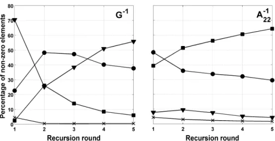
addition, for the case of A₂₂, results show that, even if the number of contributions to compute is large, a majority of these contributions are close to 0. Focusing on the determination of these contributions would be helpful to address the main question of this thesis.

Therefore, the research focuses on A₂₂ in the upcoming chapters. The core of Chapter IV is the proposal of a heuristic algorithm that exhaustively searches the pedigree to find contributors of each genotyped animal. Computations of contributions are then restricted to these contributors, as other animals do not contribute. Moreover, in Chapter IV, a strategy is proposed to reduce the number of contributors, namely to extract pedigree of genotyped animals only on few generations. Results show that inversion and approximations are very fair; however, computations still have a cubical complexity with the order of the matrix. This complexity could be avoided if the relation between the number of contributors and the matrix order would be broken or, at least, tempered.

Consequently, a restricted search for contributors is proposed in Chapter V. This algorithm – actually, a restricted version of the core algorithm of Chapter IV – allows fair and close to sparse approximations of the inverse of A₂₂ . Results show that approximations have a limited impact on the further use of the inverse of A₂₂.

Eventually, Chapter VI is a general discussion that starts by a comparative study of the different algorithms proposed for A22 and those proposed for G. For each

algorithm, an implementation is proposed and tests are ran on the same computer in order to compare time and memory efficiencies and, if required, quality of approximation. Future perspectives of research and use of the proposed algorithms are discussed and general conclusions are drawn in the last chapter (Chapter VII).

A reminder of the thesis outline takes place in front of every chapter. In addition, Chapters II to V are followed by a summary of the main results outlined in the chapter and essential to follow the strategy of research. Also, other communications related to the topic of the chapter are listed at the end of the chapter, if applicable.

Thesis framework

The thesis research was initiated by October 2009 and supported by an “Aide à la Formation-Recherche” (AFR) grant issued by the Fonds National de la Recherche Luxembourg (FNR), under the project name “NextGenGES”.

The initial objectives of this project were the following: (1) methodological contribution to the development of the next generation genomic prediction methods, and (2) application of these methods to milk composition traits. Different constraints that appeared during the project forced a shift in the thesis objectives. These constraints were: (1) the unfitness between the purpose of methodological developments (drawing solutions for large matrices) and the size of the dairy cattle population from Luxembourg; (2) the unavailability of genotypes in Luxembourg; and (3) the increasing relevance of the methodological issues that appeared during the research.

Under the terms of this grant, the research was part of a public-private partnership between the cattle society from Luxembourg CONVIS s.c. and the host institution of this doctoral thesis, Gembloux Agro-Bio Tech, part of the University of Liège (Gembloux, Belgium). The major part of the doctoral research was done at Gembloux Agro-Bio Tech, under the supervision of Prof. N. Gengler, on pedigree data provided by CONVIS s.c., where a certain time of work was also spent. In addition, a third institution was involved in the project, the Animal and Dairy Science Department of the University of Georgia (Athens, GA, USA), where the training on computational techniques in animal breeding and the first methodological researches were carried out under the co-supervision of Dr. I. Misztal.

This grant initially covered three years, it was then renewed for a fourth year in October 2012 and it eventually ended in September 2013. For the remaining period of doctoral research (October 2013 to May 2014), the work done for this thesis contributed to the project “DairySNP” done by Gembloux Agro-Bio Tech and the Walloon Breeding Association (“Association Wallonne de l’Elevage”, AWE) and supported by the Ministry of Agriculture of the Walloon Region of Belgium.

Alongside to the thesis, a doctoral formation was successfully completed. The doctoral formation included, among others, the following main aspects: attendance to classes in animal breeding and genetics and big data management, active participation to international congresses, teaching assistance of the quantitative genetics class taught in

Gembloux by Prof. N. Gengler and publication of research outputs in peer-reviewed journals.

References

Aguilar I., Misztal I., Legarra A. and Tsuruta S., 2011. Efficient computation of the genomic relationship matrix and other matrices used in single-step evaluation. J. Anim. Breed.

Genet., 128, 422–428.

Bömcke E., Soyeurt H., Szydlowski M. and Gengler N., 2010. New method to combine molecular and pedigree relationships. J. Anim. Sci., 89, 972–978.

Calus M.P.L., Meuwissen T.H.E., de Roos A.P.W. and Veerkamp R.F., 2008. Accuracy of Genomic Selection Using Different Methods to Define Haplotypes. Genetics, 178, 553– 561.

Christensen O.F. and Lund M.S., 2010. Genomic prediction when some animals are not genotyped. Genet. Sel. Evol., 42, 2.

Fernando R.L. and Grossman M., 1989. Marker assisted selection using best linear unbiased prediction. Genet. Sel. Evol., 21, 1–11.

Fisher R.A., 1918. The Correlation between Relatives on the Supposition of Mendelian Inheritance. Earth Environ. Sci. Trans. R. Soc. Edinb., 52, 399–433.

Goddard M.E., 1992. A mixed model for analyses of data on multiple genetic markers. Theor.

Appl. Genet., 83, 878–886.

Hammami H., 2009. Genotype by Environment Interaction for Production Traits of Holsteins

Using Two Countries as Model: Luxembourg and Tunisia. Gembloux, Belgium:

University of Liège.

Hazel L.N., 1943. The Genetic Basis for Constructing Selection Indexes. Genetics, 28, 476–490. Henderson C.R., 1953. Estimation of Variance and Covariance Components. Biometrics, 9, 226–

252.

Henderson C.R., 1973. Sire evaluation and genetic trends. In: Proc. Anim. Breed. Genet. Symp.

Honor Dr Jay Lush., Am. Soc. Anim. Sci. and Am. Dairy Sci. Assoc., Poultry Sci. Assoc.,

Champaign, IL, 10-41.

Henderson C.R., 1976. A Simple Method for Computing the Inverse of a Numerator Relationship Matrix Used in Prediction of Breeding Values. Biometrics, 32, 69–83.

Hickey J.M., 2013. Sequencing millions of animals for genomic selection 2.0. J. Anim. Breed.

Genet., 130, 331–332.

Legarra A., Aguilar I. and Misztal I., 2009. A relationship matrix including full pedigree and genomic information. J. Dairy Sci., 92, 4656–4663.

Meuwissen T.H.E., Hayes B.J. and Goddard M.E., 2001. Prediction of total genetic value using genome-wide dense marker maps. Genetics, 157, 1819–1829.

Misztal I., Legarra A. and Aguilar I., 2009. Computing procedures for genetic evaluation including phenotypic, full pedigree, and genomic information. J. Dairy Sci., 92, 4648– 4655.

Pearl R., 1917. Studies on Inbreeding. VII.-Some Further Considerations Regarding the

van Arendonk J.A.M., Tier B. and Kinghorn B.P., 1994. Use of multiple genetic markers in prediction of breeding values. Genetics, 137, 319–329.

VanRaden P.M., 2007. Genomic measures of relationship and inbreeding. Proc Interbull Annu.

Meet., 33–36.

VanRaden P.M., 2008. Efficient Methods to Compute Genomic Predictions. J. Dairy Sci., 91, 4414–4423.

VanRaden P.M., Null D.J., Sargolzaei M., Wiggans G.R., Tooker M.E., Cole J.B., Sonstegard T.S., Connor E.E., Winters M., van Kaam J.B.C.H.M., Valentini A., Van Doormaal B.J., Faust M.A. and Doak G.A., 2013. Genomic imputation and evaluation using high-density Holstein genotypes. J. Dairy Sci., 96, 668–678.

Whetham E.H., 1979. The Trade in Pedigre Livestock 1850-1910. Agric. Hist. Rev., 27, 47–50. Wright S., 1922. Coefficients of Inbreeding and Relationship. Am. Nat., 56, 330–338.

Chapter II

L

ITERATURE

R

EVIEW

In genetic evaluations, relationship matrices establish the covariance structure of the genetic effect; each type of genetic effect (additive, dominance…) has its own type of relationship. Mixed model equations integrate the inverse of the relationship matrix of a certain type of genetic effect in order to obtain solutions for that type of effect. Therefore, computing the inverse of a relationship matrix without having to set up the matrix itself is of great interest in order to ease evaluations. In the third section of this chapter, the main algorithms to directly compute inverses of relationship matrices are reviewed. Beforehand, in the first and second sections, the operation of inversion and the features of the two matrices of interest ( A₂₂ and G) are introduced.

Matrix inversion

A square matrix A of order n is invertible if a matrix B of same order exists such as their product returns the identity matrix of same order: AB = I = BA. B is called the inverse matrix of A and is denoted by A!1_.

Matrix A is invertible if the determinant of A is different from zero. The determinant can be computed from the values of elements in A. Moreover, the determinant of a product of matrices is the product of the determinant of each matrix. Different methods allow computing the inverse of a matrix. These methods can be categorized into direct and iterative methods.

Direct methods require high accuracy in calculation to obtain proper solutions whereas iterative methods compensate round-off errors by a process of successive refinement (Rajagopalan, 1996). The most commonly implemented method is a direct one: the Gauss-Jordan method. This method applies a sequence of transformations of rows and columns on the original matrix and an identity matrix in order to convert the original matrix into an identity matrix. The inverse is then stored in the second matrix. The Cholesky factorization of symmetric matrix (A = L !L ; Cholesky, 1910) can be used to compute its inverse by computing the inverse of L and multiplying it by its transpose. Another direct method is the Sherman-Morrison algorithm (Sherman and Morrison, 1950). This algorithm performs inversion in a line-wise manner: a zeroed matrix is updated, at each row, by the product of a vector of same length as the order of the matrix by its transpose. This vector is computed from the result of the previous inverse and the corresponding column in the original matrix. Sherman-Morrison algorithm is equivalent to the blockwise inversion algorithm (Banachiewicz, 1937) in which the Schur complement would be scalar.

Iterative methods work by successively improving approximations until a numerical convergence is reach. Speed of convergence is, however, dependent on the initial approximation. Among others, pre-conjugate gradient and bi-conjugate gradient stabilized methods are worth citing.

Additive and genomic relationship matrices between

genotyped animals

If some animals are genotyped in a population, one can split this population between genotyped and non-genotyped animals. Such a basic splitting of the original population into two groups is feasible for any feature, e.g. splitting between recorded and non-recorded animals, between sexes or between breeds.

From a partition between genotyped and non-genotyped animals, two additive relationship matrices may be computed. The first one, A₂₂, is the part of the additive relationship matrix that gathers relationships between genotyped animals. The second one,

G, is a matrix of similarities between genotyped animals computed using genomic

information. In a certain sense, G can be also be interpreted as part of a larger matrix: this larger matrix would be of the same size as A, only possible, however, if genomic information was available for all animals in population.

Additive relationship matrix between genotyped animals

Additive relationships coefficients are relationship measurements based on the knowledge of potential co-ancestries between two animals. Setting up such relationship coefficients requires having genealogical information, often streamlined in a table of triplets animal-sire-dam. Such table, as well as any triplet it contains, is called “pedigree”.

The additive relationship coefficients are due to Wright (1922) and have a range in

0, 2

[

[

The relationship coefficient of an animal with itself is defined as 1 plus the inbreeding coefficient of that animal. The inbreeding coefficient (F) is the half of the relationship coefficient between the two parents.

Matrix A is symmetric and positive-definite. Non-singularity of A can be proved using the rules to compute the diagonal elements (Quaas, 1976) of its Cholesky factorization (see Henderson, 1976) and using the definition of additive relationship coefficients. For an animal with both parents known, the diagonal element of the Cholesky factorization is

(

)

inbreeding coefficients of the sire and the dam of that animal. Inbreeding coefficients are the half of relationship coefficients and therefore have a range from 0 to 1 excluded. Consequently, the diagonal element of the Cholesky factorization is always positive, allowing existence of that factorization and non-singularity of the matrix. Inversion of A is detailed further in this chapter.

Matrix A22 is any part of A gathering relationship coefficients between animals

chosen among all animals in population. In our case, this group is the group of genotyped animals. Matrix A22 has therefore the same structure and properties as A. The quickest

and simplest way to compute A₂₂ is the method of Colleau (2002). This method is derived from the inverted Cholesky factorization of A and it computes the additive relationship coefficients of an animal with the rest of the population by a double reading of an age-ordered pedigree. Applying the method for all genotyped animals and retaining only relationships with genotyped animals achieves computation of A₂₂.

Genomic relationship matrix

Genomic relationship coefficients are relationship measurements based on similarities between individuals revealed by molecular markers.

Nejati-Javaremi et al. (1997) were the first to outline a method to derive the allelic relationship TA between two individuals x and y at a given locus l: they averaged the identity between the two alleles of an individual at this locus and both alleles of another individual at the same locus. The measure is repeated for all L available marker loci and averaged, returning the total allelic identity between the two individuals (equation II.1).

TAxy = TAl l=1 L

!

This method was, among others, implemented by Bömcke and Gengler (2009), using 16 microsatellites markers with at least 4 alleles, in order to derive a combined pedigree-genomic additive relationship.

The development of genome sequencing methods made hundreds of thousands of single nucleotide polymorphisms (SNP) available, opening the path to genomic selection (Meuwissen et al., 2001; Goddard and Hayes, 2007). Among the large number of SNP widely spread over the genome, bi-allelic markers are chosen to create assays of several

thousands of SNPs (3,000, 10,000 or 50,000 on the most used beadchips). This availability considerably increased the accuracy of the relationship measurement, as well as its simplicity because SNPs are bi-allelic. Using bi-allelic genotypes (-1 and 1 for both homozygotes; 0 for heterozygote) in equation (II.1), one can define a matrix of total allelic relationship as in equation (II.2), where Z0 is a matrix containing, in row, bi-allelic

genotypes and, in column, m SNPs.

TA =Z0Z!0+ m

m (II.2)

However, at a given locus, if an allele is less frequent than the other one, two individuals carrying this allele are more likely to be related than two animals carrying the frequent allele. In other words, common alleles are less informative than rare alleles to compute relationships. Thus, taking allelic frequencies into account matters.

VanRaden (2007) proposed a genomic relationship matrix (equation II.3) structurally similar to that derived (equation II.2) from Nejati-Javaremi et al. (1997), but that accounts for allelic frequency in both the genomic incidence matrix (Z) and the scaling factor (d).

G =Z !Z

d (II.3)

Matrix Z is obtained by subtraction of P from Z₀. Each row of P contains the allelic frequencies of all alleles expressed as a difference from 0.5 and multiplied by 2, so that the i-th column of P is2 f

(

)

SNP. As explain in VanRaden (2008), subtracting P from Z₀ gives more credit to rare alleles than to common alleles. The scaling factor d is equal to 2

"

according to VanRaden (2008), makes G analogous to A22. This analogy has to be

tempered for two reasons. Firstly, tuning is required to make both diagonal and off-diagonals values compatible with A₂₂ (see Forni, 2011). Secondly, matrix A₂₂ measures identity-by-descent (IBD) between animals whereas matrix G measures identity-by-state (IBS) between animals. IBS can be imputed either to co-ancestry or to randomly occurring mutations. Recent proposals create G-IBD matrices by tracing the gene flows through pedigrees (Villanueva et al., 2005) or using haplotypes (Hayes et al., 2009).

Matrix G (equation II.3) is positive semi-definite (VanRaden, 2007) but can be singular if two clones are genotyped, or if identical genotypes are found for two different animals because the number of SNPs is small. In such case, the pairs of rows and columns corresponding to these animals are the same. Also, matrix G can be singular if the total number of alleles is less than the number of genotyped individuals. Using a combined G made of a high proportion of G and a low proportion of A22 could circumvent

singularity.

Even though, in this study, G is used as defined in equation (II.3) and made compatible with A₂₂ using methods by Forni (2011), other genomic relationship matrices are worth citing (Leutenegger et al., 2003; Amin et al., 2007; Gianola and van Kaam, 2008).

Techniques for inversion of relationship matrices

[FROM: P. Faux and N. Gengler. 2014. A review of inversion techniques related to the used of relationship matrices in animal breeding. Biotechnologie, Agronomie, Sociétés et Environnement, (in press)]

Abstract

In animal breeding, prediction of genetic effects is usually obtained through the use of mixed models. For any of these genetic effects, mixed models require the inversion of the covariance matrix associated to that effect, which is equal to the associated relationship matrix times the associated component of the genetic variance. Given the size of many genetic evaluation systems, computing the inverses of these relationship matrices is not trivial. In this review, we aim to cover computational techniques that ease inversion of relationship matrices used in animal breeding for prediction of the following different types of genetic effects: additive effect, gametic effect, effect due to presence of marked quantitative trait loci, dominance effect and different epistasis effects. Construction rules and inversion algorithms are detailed for each relationship matrix. In the final discussion, we draw up a common theoretical frame to most of the reviewed techniques. Two computational constraints come out of this theoretical frame: setting up the matrix of

dependencies between levels of the effect and setting up some parts (diagonal or block-diagonal elements) of the relationship matrix to be inverted.

Keywords: animal breeding, quantitative genetics, breeding value.

Introduction

A simple model (equation II.4; see Kempthorne, 1955) describes a given phenotype (P) as the sum of the genotype (G) and the environment (E) of a particular animal.

P = G + E (II.4)

Based on equation (II.4), variations among phenotypic observations are therefore explained by genetic and environmental variations and by a potential interaction between genotype and environment. Genetic improvement of animals requires accurate estimation of the genetic variance component in order to predict the genetic values of animals. The structure of this variance component is based on knowledge of the biological processes involved in Mendelian inheritance.

In nearly all domestic species, animals have a diploid genome (with the exception of honey bees, where males are haploid). Then, during the production of gametes, a haploid copy of the diploid genome of the original animal (sire or dam) is made. However, haploid copies are produced from potentially different parts of the homologous chromosomes, following the process of recombination due to crossing-over. Thus, for any locus, a gamete carries a single copy of one of the two alleles carried by the parental genome. Both gametes eventually merge to create a new animal.

By the process described before, every new animal has a specific and unique genetic makeup. Genetic covariances among different animals arise because they have inherited similar alleles and allele combinations. Based on these covariances, associations among these animals can be defined as ratios between covariances and variances associated to a given genetic effect. Whether the interactions between alleles of the same locus (intra-locus interaction) and between loci (inter-loci interaction) are null or not, several types of genetic effects can be distinguished. In our study, we will cover and detail the following genetic effects: additive, gametic, effect due to marked QTL, dominance and the different types of epistasis effects.

When fitting a linear model with generalized least squares, use of the inverted covariance structure among observations allows obtaining Best Linear Unbiased Estimators. Prediction of genetic effects is usually obtained through the use of mixed models (Henderson, 1953; Henderson, 1973). These models are equivalent to models fitted using generalized least squares and, for every random effect, the inverse of the associated covariance structure is also needed.

Due to huge size of regular genetic evaluations, there is a substantial interest in computational techniques that make efficient use of covariance matrices in terms of computing time and memory requirements. Thus, our main objective is to review and explain in detail algorithms for inversion of relationships matrices useful in animal breeding. Completion of this objective involved the definition of the relationships between levels of the concerned genetic effect and the computation of the related matrices for each type of genetic effect listed above (additive, gametic, marked QTL effects, dominance and epistasis). Finally, we outline a general framework of inversion of relationship matrices in the final discussion.

It must be noted that the case of genomic relationship matrices has been willingly discarded in this study because no algorithm that directly sets up their inverses has been developed so far. The genomic relationships are made available by the use of dense marker chips (over than tens of thousands of markers) and give an accurate estimation of the observed relationship between two animals. For their computation, please refer to the work of VanRaden (2008), for additive genomic relationship matrix, and Su et al. (2012) for non-additive genomic relationship matrix.

Additive relationship matrix

Definition of the additive relationship

If interactions between alleles are considered null, the genetic (co)variance is said to be “additive”. Based on previous work by Pearl (Pearl, 1917a; Pearl, 1917b), Wright (1922) defined an additive relationship coefficient as the additive correlation between two animals i and j (equation II.5).

rij= Cov i, j

_{[ ]}

_{[ ]}

_{[ ]}

The rij coefficient is a correlation coefficient; it ranges from 0 to 1. The

non-scaled coefficient of Wright, noted a_ij, is the additive genetic relationship coefficient and, from (II.5), is defined as equal to r_ij a_ii! ajj . This coefficient is also often referred as the

“numerator relationship” coefficient (due to its position in equation II.5). We will denote it as the “additive relationship coefficient” and the kind of relationship that it refers to as an “additive relationship” in our study. The matrix containing all these additive relationship coefficients will be denoted by A and called “additive relationship matrix”.

Computation of the additive relationship matrix

Complete computation of the additive relationship matrix

The path coefficient method (Wright, 1922) enables the computation of the additive relationship between two animals. The process requires identification of all nearest ancestors shared between those two animals and counting of the number of generation steps between them. The path coefficient method can be automated and extended to computation of relationship coefficients in the whole population. The tabular method (Emik and Terrill, 1949; Henderson, 1976) performs the computation of additive relationship coefficients in a recursive manner. For a given animal, the relationship coefficients of this animal with all older animals are computed in a row by adding one half of the relationship coefficients in the rows of its parents. A prior step is required: organization of pedigree records in a sorted by generation list of triplets animal-sire-dam (Emik and Terrill, 1949; Mugnier et al., 1966). On a population of n animals, a square matrix of order n is created.

This algorithm has a complexity that is proportional to n2, because, at each of the n loops it achieves, a linear combination of a vector of maximum length n is performed. Storage requirements follow the same trend and may quickly become prohibitive.

Partial computation of the additive relationship matrix

For this reason, and also because only a section of the additive relationship matrix may be of interest in large populations, algorithms that permit a partial computation of the additive relationship matrix have been developed.

Algorithms corresponding to two specific parts of the A matrix should be mentioned. The first one is an algorithm that computes the relationship coefficients of a particular animal with the rest of the population (e.g. Colleau, 2002). The second one is an

algorithm that computes the diagonal elements of A, which reveals inbreeding coefficients (e.g. algorithms of Quaas, 1976; Meuwissen and Luo, 1992; Sargolzaei et al., 2005). The interest of these coefficients will be highlighted in the next sections.

Computation of the inverse of the additive relationship matrix

Matrix A is non-singular except in the presence of genetically identical animals (GIA; full-twins or clones). In such situations, contributions of Kennedy and Schaeffer (1989) and Oikawa and Yasuda (2009) are relevant.

In situations without GIAs, Henderson (1976) has proposed rules that allow computing the inverse of A without having to compute A explicitly. These rules are based on the simplicity of structure of matrices involved in the factorization of A: A = TD !T . According to Henderson (1976), matrix T can be computed recursively (equation II.6): the vector corresponding to the i-th row of T, from column 1 to (i-1), is equal to one half of corresponding parental vectors (say s and d). Diagonal value is 1 and upper triangular part is 0. T_(i)= T_(i!1) 0 0 p" T_{(i) (i!1)} 1 ! 0 " 0 # $ % % % % % & ' ( ( ( ( ( , where p_(i)! = 0 ! 0.5" s ! 0.5d 0 # $ $ % & ' ' (II.6)

Inverting the factorization of A and using it to compute the inverse of A (as (T!1

"

) D!1_T!1) does not require T, but the inverse of T. This latter has a very simple

structure that comes by inversion of a triangular matrix (equation II.7).

T(i) !1 = T_(i!1)!1 ₀ 0 !p"(i) 1 ! 0 " 0 # $ % % % % % & ' ( ( ( ( ( (II.7)

The matrix D is diagonal: element Dii is equal to 1!.25" App

#p$%i

&

denotes the set of known parents (either 0, 1 or 2 parents known) of animal i. A correct computation of D requires to know the diagonal elements of A. Algorithms for computation of inbreeding coefficients mentioned in section “Computation of the additive

Quaas (1976) is noteworthy as it is the first one to compute these elements for the particular purpose of the computation of the inverse of A.

Once matrix D has been computed, Henderson (1976) proposed a simple algorithm to set up the inverse (Algorithm II.1). The algorithm summarizes the product

(T!1

"

) D!1_T!1 to n updates of a n-by-n matrix that was initially set to zero. Each update is a

square block matrix of order 1 plus the number of known parents. This principle was demonstrated in Tier and Sölkner (1993) and van Arendonk et al. (1994).

Algorithm II.1. Direct computation of the inverse of the additive relationship matrix (A). initialize B = D!1 _{and A}!1

= B, two matrices of order n

for i = 1 to n, do

if any parent, say p, of the i-th animal is known, then add !.5Bii to elements Api

!1 _{and A}

ip

!1 _and

.25Bii to element App

!1

if both parents, say p and q, of the i-th animal are known, then add .25Bii to elements Apq

!1 _{and A}

qp

!1

The advantages of this algorithm are its low complexity (O(n)) and the low amount of memory required to store the very sparse output (A!1_).

Gametic relationship matrix

Definition and uses of gametic relationships

In some situations, it may be interesting to express the additive genetic value of an individual in terms of the separate gametic contributions of each of their two parents (Schaeffer et al., 1989; Kennedy et al., 1988). Prediction of additive gametic values instead of additive genetic values allows reducing the size of the system to solve: the number of genetic effects is equal to the number of parents, necessarily lower than the total number of animals in the population. The covariance matrix used for random genetic (gametic) effects is called the “gametic relationship matrix” and denoted hereafter as Ga. Quaas and Pollak (1980) have developed such a model, known as reduced animal model. This model also shows how each ancestor affects the genetic value of the individual. Gibson et al. (1988) have proposed a gametic model in which only one parental gamete expresses the genetic effect (autosomally inherited) of an individual. Others uses are:

analysis of haploid-diploids species such as the honey bee (Smith and Allaire, 1985) and analysis of gametic imprinting effects (Gibson et al., 1988; Schaeffer et al., 1989). Eventually, the usefulness of the gametic relationship matrix in computation of the dominance relationship matrix has been shown by Schaeffer et al. (1989). The derivation of A from the gametic relationship matrix has been described by Smith and Allaire (1985) and showed by Jamrozik and Schaeffer (1991). Matrix A is obtained by 1

2KG !K , where

K = I ! 1 1"_# $_% (Tier and Sölkner, 1993; van Arendonk et al., 1994).

Computation of the gametic relationship matrix

Smith (1984) proposed an algorithm to compute G_a that is inspired by the tabular method. For diploids species, the size of the matrix will be N = 2n, where n is the number

of animals in population. Each animal has thus two rows/columns that correspond to both parental gametes. Construction rules are simply deduced from the tabular method: if the parent p is known, then the row elements below diagonal are equal to the half of the sum of corresponding elements in both lines of parent p; else if the parent p is unknown, these elements are null. The corresponding column is obtained by transposition.

Inversion of the gametic relationship matrix

Matrix G_a is non-singular within the same restriction as for matrix A (no clones). The following algorithm (Algorithm II.2) was developed by Schaeffer et al. (1989) based on direct computation of the inverse of A. Animals are supposed to be ordered chronologically. For each animal, the first and second gametes are respectively due to the sire and dam. Computation of the diagonal elements is similar to that of Quaas (1976).

Algorithm II.2. Direct computation of the inverse of the gametic relationship matrix (Ga) due to Schaeffer et al. (1989).

initialize a matrix G_a!1 _{of order N and three vectors u, v and d of length N}

for k = 1 to N, do

set d(k) = v(k) = 1! u(k)

if the k-th gamete precedes any parental gamete, say p, of the i-th gamete, then add .5v(p) to v(i)

else set v(i) equal to 0

add the square of v(i) to u(i)

set c equal to the square of the inverse of d(k) and G_a!1

(k, k) equal to c

if parental gametes, say p and m, of the k-th gamete are known, then add !.5c to G_a!1_{( p, k), G} a !1_{(m, k), G} a !1_{(k, p) and G} a !1_{(k, m)} add .25c to G_a!1 ( p, p), Ga !1 ( p, m), Ga !1 (m, p) and Ga !1 (m, m)

Covariance matrices for marked QTL effects

Definition of marked QTL covariance

Development of genetic engineering techniques leads to identify loci involved in determinism of quantitative traits (QTL) and to assist selection by use of markers linked to these QTL (Marked QTL, MQTL; Soller and Beckmann, 1983; Smith and Simpson, 1986). The following model (Fernando and Grossman, 1989) integrates effects of a causative QTL into BLUP.

yi = x!" + vi i p

+ vi m

+ ui+ ei (II.8)

In equation (II.8), a phenotypic value y_i is decomposed in environmental contributions x!i", random additive genetic contributions: a contribution of the paternally

inherited allele of a marked QTL ( v_ip_{), a contribution of the maternally inherited allele of}

the same marked QTL ( v_im_{) and a residual additive contribution due to QTLs unlinked to}

the marker (ui), and a random error contribution (ei). Solving this mixed model requires

the covariance matrix of the vi values (called “MQTL matrix” and denoted as G

hereafter), which is computed using both pedigree relationships and marker information.

Computation of the MQTL matrix

Fernando and Grossman (1989) have developed the “MQTL relationship” in a similar manner as the additive relationship. While this latter is based on the probability that alleles at a same locus for each animal are IBD, MQTL relationship is based on the conditional probability of the same event given information on a marker closely linked to