HAL Id: tel-00959330
https://tel.archives-ouvertes.fr/tel-00959330
Submitted on 14 Mar 2014
HAL is a multi-disciplinary open access
archive for the deposit and dissemination of sci-entific research documents, whether they are pub-lished or not. The documents may come from teaching and research institutions in France or abroad, or from public or private research centers.
L’archive ouverte pluridisciplinaire HAL, est destinée au dépôt et à la diffusion de documents scientifiques de niveau recherche, publiés ou non, émanant des établissements d’enseignement et de recherche français ou étrangers, des laboratoires publics ou privés.
Jinglin Zhang
To cite this version:
Jinglin Zhang. Prototyping methodology of image processing applications on heterogeneous parallel systems. Other. INSA de Rennes, 2013. English. �NNT : 2013ISAR0035�. �tel-00959330�
Prototyping methodology of
image processing
applications on
heterogeneous parallel
systems
Thèse soutenue le 19.12.2013devant le jury composé de :
Michel PAINDAVOINE
Professeur des Universitésà l'Université de Bourgogne / Président
Dominique HOUZET
Professeur des Universités Grenoble-INP / Rapporteur
Guillaume MOREAU
Professeur des Universités Centrale Nantes / Rapporteur
Jean-Gabriel COUSIN
Maître de conférence à l'INSA de Rennes / Co-encadrant
Jean-François NEZAN
Professeur des Universités à l'INSA de Rennes / Directeur de thèse
THESE INSA Rennes sous le sceau de l’Université européenne de Bretagne
pour obtenir le titre de
DOCTEUR DE L’INSA DE RENNES
Spécialité : Electronique et télécommunications
présentée par
Jinglin ZHANG
ECOLE DOCTORALE : MatissePrototyping methodology of image processing
applications on heterogeneous
parallel systems
Jinglin ZHANG
Thank Prof. Jean-François Nezan!
Thank Dr. Jean-Gabriel COUSIN!
Thank China Scholarship Council!
Thank my father, ZHANG Dazeng!
Thank my mother, WANG Xiuling!
Thank my wife, TAN Huiwen!
Thank my son, ZHANG Tanyixi!
The work of this thesis is one three-years work and life in INSA-Rennes. It is also a very important part in my life. In here, i have learned how to make research. First, i would like to thank my advisors Prof. Jean-François Nezan and Associate Prof. Jean-Gabriel Cousin for their help, suggestion and encouragement, for the time they spent to correct my papers and this PHD thesis. I don’t forget that Jean-François revise my first conference paper again and again although he is very busy. I also remember that Jean-Gabriel teaches me to make some slides and to present my work. In particular, i thanks Matthieu Wipliez and Mickaël Raulet who helped me to debug the code when i was falling down with programming. I thanks Jean-François give me such a opportunity to study and make research here. I also thank China Scholarship Council to support my scholarship of 48 months living in Rennes, France.
Three year almost thousand days in our laboratory is quite a long time. I thank all the colleague Matthieu Wipliez, Nicloas Siret, Maxime Pelcat, Jérôme Gorin, Mickaël Raulet, Karol Desnos, Hervé Yviquel, Antoine Lorence, Khaled Jerbi, Julien Heulot, Erwan Raffin, who help me in the research and daily life. I enjoyed the laboratory life and its friendly environment, although i didn’t communicate too much with you owing to my poor french speaking. Thanks you Hervé, have helped me making a phone call for house-hunting and something else. Maxime Pelcat, thank you being a listener and advisor in my presentations, also helping me to present the slides in the Dasip13 conference. Thanks Alexandre MERCAT’s work on stereo matching on MPPA platform. Thanks to Aurore Gouin and Jocelyne Trenmier for managing administrative works.
I am grateful to all my friends, my Chinese colleagues. Yi Liu, Wenjing Shuai thank you for being my models in my experiment tests. Cong Bai, Ming Liu thank you for giving me the suggestions to revise papers and the templet of Ph.D thesis. Fu Hua thank you for helping me to write the abstract of French. Thank you all
7
the guys who invited me and prepared the meals almost every weekend when i was alone without my families.
Thank you, my wife Huiwen Tan, for taking care of our son Yixi. I apologize that i cannot live with you and take care of you in the more than three years. Although you always quarrel with me, i thank a lot because of your effort for our family, i am not a good husband and father until now. For my parents, father Dazeng Zhang, mother Xiuling Wang, thank you raising me up and teaching me when i was young. I can only to say i love you.
Contents
Contents 9 1 Introduction 13 1.1 Context . . . 13 1.2 Contributions . . . 17 1.3 Road Map . . . 19 2 Background 21 2.1 Target Architectures . . . 212.1.1 CPU and GPU . . . 23
2.1.2 Platform MPPA Kalray . . . 23
2.2 OpenCL: An Intermediate Level Programming Model . . . 24
2.3 The Dataflow Approach: An High Level Programming Model . . . 29
2.3.1 Definition of reconfigurable video coding . . . 30
2.3.2 Dataflow models of computation . . . 31
2.3.3 Dataflow sigmaC . . . 34
2.3.4 RVC-CAL language . . . 34
2.4 Tools of Rapid Prototyping Methodology . . . 38
2.4.1 Orcc, an Open RVC-CAL Compiler . . . 39
2.4.2 Preesm, a Parallel and Real-time Embedded Executives Schedul-ing Method . . . 40
2.4.3 HMPP, a Hybrid Multicore Parallel Programming model . . . 40
2.5 Concerned Image and Video Processing Algorithms . . . 42
2.5.1 Motion estimation . . . 43
2.5.2 Stereo matching . . . 44
2.6 Conclusion . . . 47
3 Parallelized Motion Estimation Based on Heterogeneous System 49 3.1 Introduction . . . 49
3.2 Parallelized Motion Estimation Algorithm . . . 53
3.2.1 SAD computation . . . 55 9
3.2.2 SAD comparison . . . 56
3.3 Optimization Strategies of Parallel Computing . . . 57
3.3.1 Using shared memory . . . 57
3.3.2 Using vector data . . . 58
3.3.3 Compute Unit Occupancy . . . 59
3.3.4 Experimental Result . . . 59
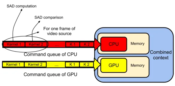
3.4 Heterogeneous Parallel Computing with OpenCL . . . 63
3.4.1 Cooperative multi-devices usage model . . . 63
3.4.2 Workload distribution . . . 64
3.4.3 Find the balance of performance . . . 65
3.5 Rapid Prototyping for Parallel Computing . . . 66
3.5.1 CAL Description of Motion Estimation . . . 67
3.5.2 Analysis of experiments result . . . 68
3.6 Conclusion . . . 70
4 Real Time Local Stereo Matching Method 71 4.1 Introduction . . . 71
4.2 Proposed Stereo Matching Algorithm . . . 77
4.2.1 Combined cost construction . . . 77
4.2.2 Proposed cost aggregation method . . . 79
4.2.3 Disparity selection . . . 82
4.2.4 Post processing of disparity maps . . . 82
4.2.5 CAL description of stereo matching . . . 84
4.3 Experimental Result and Discussions . . . 85
4.3.1 Matching accuracy . . . 86
4.3.2 Time-efficiency results . . . 88
4.3.3 Proposed stereo matching method with SigmaC dataflow . . . 89
4.4 Conclusions . . . 90
5 Joint Motion-Based Video Stereo Matching 91 5.1 Introduction . . . 91
5.2 Joint Motion-Based Stereo Matching . . . 92
5.2.1 Local support region building . . . 92
5.2.2 Combined raw cost construction . . . 96
5.2.3 Gaussian adaptive support weights . . . 97
5.2.4 Proposed cost aggregation . . . 98
5.2.5 Disparity determination . . . 99
5.3 Video Stereo matching Implementation with Heterogeneous System . 99 5.4 Evaluation and Discussions . . . 100
5.4.1 Matching accuracy . . . 100
5.4.2 Time-efficiency results . . . 102
5.5 Stereo Matching Graphical User Interface (GUI) . . . 102
5.6 Conclusions . . . 106
6 Conclusion and Perspective 107 6.1 Conclusion . . . 107
Contents 11
A Résumé étendu en français 111
List of Figures 139
Publications 144
1
Introduction
1.1 Context
Inspired and motivated by the conclusion made by Gordon Moore in 1965, the density of transistors in a chip was doubled every 18 months. More transistors allow more complex chip-designs, and smaller transistor allows a higher frequency per watt consumed. But there is no more increasing about clock rates because of power consumption. In order to keep the performance increment, modern processors apply a many-cores strategy instead of frequency increment.
In the meantime, image and video applications such as video coding and ultra-resolution display with novel features whose aim is to recover a real world for users from the digital world are becoming more and more complex. Thereby, the need for computational power is rapidly increasing. The accuracy and the time-efficiency are two key criterions in the image and video processing applications. Better quality can be achieved by using more sophisticated algorithms, which also means the more computational power.
All these changes make electronic manufactures developing parallel embedded heterogeneous systems which combine with different subsystems optimized to ex-ecute different workload. The tradeoff between accuracy and time-efficiency will benefit from technology revolutions of the embedded heterogeneous system and parallel computing. Some heterogeneous systems consist of Central Processing Unit (CPU), Graphics Processing Unit (GPU), and Field-programmable gate ar-ray (FPGA). GPU with herds of Processing Element (PE) is the typical case which
benefits form many core revolutions that considered as special-purpose hardware for graphical computations until the turn of the century. In fact, GPU could employ general-purpose computation in many arithmetic computation domains. There are some successful attempts for general-purpose computing in heterogeneous systems. Even if they are so less mature and much more difficult to use for terminal users and to develop for researchers. With their immense processing power, GPU can be orders of magnitude faster than CPUs for numerically intensive algorithms that are designed to fully exploit the parallelism available. Lately, the interest in parallel programming has grown even more in popularity because of the availability of many core devices. The General-Purpose Graphics Processing Unit (GPGPU) research field has extended to the fields as diverse as artificial intelligence, medical image processing, physical simulation and financial modeling.
When the heterogeneous computing system became the trend of the hardware design and development in the domain of image and video processing, some par-allel embedded System on Chips (SoC) like NVIDIA’s Tegra, MediaTex’s MT and Qualcomm’s Snapdragon series comes up with a high speed development of per-sonal portable devices like smartphone, TabletPC (Tablet Perper-sonal Computer) and so on. For these terminal users, parallel embedded heterogeneous systems bring better performance of applications and better user experience; For these researchers and programmers, most of the heterogeneous systems allow to select the best ar-chitecture for different demands of task or the best performance for fixed tasks. However developing software for heterogeneous parallel system is considered to be a non-straightforward task.
With so much heterogeneities, developing efficient solutions and applications for such a wide range of architectures faces a great challenge. In such heterogeneous systems, there are a huge diversity in hardware architectures and configurations. Meanwhile, these electronic manufacturers provide their standard and development environment for their heterogeneous systems like AMD’s Streaming Programming Language: Brook, NVIDIA’s Compute Unified Device Architecture (CUDA) and IBM’s Unified Parallel C (UPC) and so on. But these tools and corresponding programming languages only support on their specified devices, are not compatible
1.1. Context 15 Algorithm Architecture scenario Algorithm Transformations Architecture Transformations Scheduling Simulation Code Generation Exporting Results Rapid Prototyping
Figure 1.1: Rapid Prototyping framework
for other company’s devices. In order to support different devices and different levels of parallelism, Open Compute Language (OpenCL) was proposed by Apple, NVIDIA, AMD, and IBM since 2009 year. OpenCL’s standard provides the same Application Programming Interface (API) to manage multi-devices in the combined context and to distribute the global workload to these different devices. Although there are parallel computing programming language: CUDA and OpenCL, desinging the kernel code of CUDA and OpenCL is still a complex and troublesome procedure. Implementing complex applications on such the same complex platforms have already been proven to be a daunting task. Under this context, there is a growing interest in adaptive/reconfigurable platforms that can dynamically adapt themselves to support or provide more flexible configuration and better performance for the ap-plication. A possible answer is to follow a model based approach, where both the hardware platform and the application are abstracted through models. These models are used to capture a given domain-specific knowledge into a formal abstract rep-resentation. Models of Computations (Kahn Process Network (KPN), Synchronous Dataflow (SDF), etc.) specify the behavior of a system and are a perfect example of such an abstraction. Similarly, platform models which abstract the hardware com-ponents of a system (processing resources, communication, etc.) are also a common abstraction for embedded platform designers. However, in spite of some early work done in this direction, there is currently still no modeling approach taking run-time adaptation into consideration (from both a hardware and software point of view).
A prototyping methodology is a software development process which allows de-velopers to create portions of the solution to demonstrate functionality and make needed refinements before developing the final solution. The goal of rapid prototyp-ing framework is to propose generic models for adaptive multi-processors embedded systems. Figure 1.1 describes a global view of rapid prototyping framework, there are lots of attempts and research works around this goal. Basically, our rapid pro-totyping framework contains:
1. Dataflow Models.
2. Model to Models transformations.
3. Friendly Graphical User Interface (GUI). 4. Backend for code generation
As a consequence, Conception Orientée Modèle de calcul pour multi-Processeurs Adaptables (COMPA) project is proposed by Institut d’Electronique et de Télécom-munications de Rennes (IETR), Institut de Recherche en Informatique et Systèmes Aléatoires (IRISA), Modaë Technologies, CAPS Entreprise, Laboratoire des Sciences et Techniques de l’Information-de la Communication et de la Connaissance (Lab-STICC), Texas Instrument France in 2011. The project addresses several issues related this challenge:
– It proposes to rely on a target independent description of the application, particularly focusing on dataflow Model of Computations (MoC) and espe-cially the CAL language [1], developed in the Ptolemy project (Berkeley). The COMPA project will extend it with constructs for efficient modeling of multi-dimensional dataflow networks.
– To offer additional opportunities for optimizing the application implementa-tion, it proposes to develop a static analysis toolbox for detecting underlying MoCs used in a given CAL description. This analysis will be coupled to opti-mizing transformations on CAL models.
– It specifies and develops a "Runtime Execution Engine" which will be in charge of the execution of the CAL network on the platform. Providing runtime execution and reconfiguration services imply solving many problems including
1.2. Contributions 17
task-mapping, scheduling, etc. These problems themselves will not only take advantage of knowledge of the target architecture but also from meta data embedded in the CAL network description.
In the COMPA, three tools are proposed: the Open RVC-CAL Compiler (Orcc) [2], the Parallel and Real-time Embedded Executives Scheduling Method (Preesm) [3], and Hybrid Multicore Parallel Programming (HMPP) [4]. Orcc includes an RVC-CAL textual editor, a compilation infrastructure, a simulator and a debugger. Lots of works have been done with the Orcc and many backends are supported in the Orcc like C, C++, VHDL, HMPP and so on [5] [6] [7]. PREESM tool offers a fast prototyping tool for parallel implementations used in many applications like LTE RACH-PD algorithm and so on [8] [9] [10]. HMPP is a directive-based compiler to build parallel hardware accelerated applications. Previous research works with Orcc and Preesm was to evaluate the full prototyping framework developed in COMPA with video decoders. But video decoders are usually based on the same dataflow, the same structure with a lot of data dependencies which are very hard to map with parallelism and to implement on many core heterogeneous systems. Recently investigated motion estimation and stereo matching algorithm have the high nature of parallelism which can fully make use of the parallelism of target architectures. They are much more suitable to evaluate the efficiency of the rapid prototyping framework developed in COMPA.
1.2 Contributions
The goal of my Ph.D thesis was to evaluate and to improve the prototyping methodology for embedded systems, especially based on the dataflow modeling ap-proach (high level modeling of algorithm) and OpenCL apap-proach (intermediate level of algorithm). The first contribution of this thesis is to participate to the develop-ment of the rapid prototyping framework of COMPA project, as shown in Figure 1.2. I described the proposed motion estimation and stereo matching methods with RVC-CAL language. This rapid prototyping framework mainly contains three levels from up to down view: high level programming model, intermediate level
program-
RVC-CAL DPN
Orcc
Classify Convert Generate
HMPP Preesm
PSDF C
C with directives
Compiler ArchiModel OpenMP OpenCL
CUDA EmbeddedRuntime Embedded C
User High level programming model Intermediate level programming model Code executable on hardware
Figure 1.2: Proposed prototyping methodology in COMPA project .
ming model, code executable on hardware which will be detailed in the next chapter of background. With the aid of the Orcc, Preesm, and HMPP, it can generate and verify C/OpenCL/CUDA code on heterogeneous platforms based on multi-core CPU and GPU platforms. Obviously there are two branches in this framework. One branch is CAL → Orcc → HMP P → GP U(OpenCL/CUDA) based on the HMPP backend research of Antoine Lorence and Erwan Raffin, the another one is CAL → Orcc → P reesm → DSP/ARM(EmbeddedC) based on research work of Maxime Pelcat and Karol Desnos. My research work as part of COMPA project was to rebuild the image and video algorithms with high-level descriptions, to ver-ify the code generation. In the end, i target to the CPU, GPU and Multi-Purpose Processor Array (MPPA) of KALRAY as destination architectures to implement my applications.
1.3. Road Map 19
image and video processing algorithms:
– The proposed parallelized motion estimation (chapter 3) aims at heterogeneous computing system which contains one CPU and one GPU. I also developed one method to balance the workload distribution on such heterogeneous parallel computing system with OpenCL.
– The proposed real-time stereo matching method (chapter 4) adopts combined costs and costs aggregation with square size step to implement on an entry-level laptop’s GPU platform. Experimental results show that the proposed method outperforms other state-of-the-art methods about tradeoff between matching accuracy and time-efficiency.
– The proposed joint motion-based video stereo matching method (chapter 5) makes use of the motion vectors calculated from our parallelized motion esti-mation method to build the support region for video stereo matching. Then it employs the proposed real-time stereo matching method to process these frames of stereo video as static paired images. Experimental results show that this method outperforms these state-of-the-art stereo video matching methods in the test sequences with abundant movement even in large amounts of noise.
1.3 Road Map
The content of this thesis are structured as follows: the fundamental concept of rapid prototyping framework and the images processing algorithms concerned in our approaches are introduced in chapter 2. Approach of parallelized motion estimation based on heterogeneous computing system is presented in chapter 3 while one new accurate method to distribute the workload in video applications based on heterogeneous computing system is proposed. Approach of real time local stereo matching is elaborated in chapter 4. Approach of joint motion-based video stereo matching is detailed in chapter 5 where one new method with joint motion vector to build the support region for stereo video matching is proposed. A conclusion will be given at chapter 6.
2
Background
This chapter gives an overview of our rapid prototyping methodology from down to up view. It describes the parallel embedded systems, parallel programming mod-els, and the rapid prototyping methodology. The difference of embedded systems is discussed in the section of target architectures. OpenCL is presented as the inter-mediate level programming model in our rapid prototyping methodology. Dataflow approach is presented as the high level programming model in this methodology. Some tools used in this methodology are also introduced.
This chapter naturally begins by a presentation of target architectures in section 2.1; Section 2.2 introduces the intermediate level programming model - OpenCL; Section 2.3 presents the Dataflow approach in our rapid prototyping framework; section 2.4 presents some tools of rapid prototyping methodology. Section 2.5 intro-duces the concept of Motion Estimation and Stereo Matching algorithms; A brief conclusion is presented in section 2.6.
2.1 Target Architectures
Many core architectures like CPU, GPU, FPGA and DSP raised problems in terms of application distribution, data transferring and task synchronization. These problems become more and more complex and result in the loss of development time. Flynn’s taxonomy [11] is the most popular classification of computer architecture which defines four categories of computer architecture according to the concurrency of instruction and data streams as shown in Figure 2.1. The categories are listed as
follows:
– Single Instruction, Single Data stream (SISD) – Single Instruction, Multiple Data stream (SIMD) – Multiple Instruction, Single Data stream (MISD) – Multiple Instruction, Multiple Data stream (MIMD)13-8-25 Flynn's taxonomy - Wikipedia, the free encyclopedia
en.wikipedia.org/wiki/Flynn%27s_taxonomy 2/4
D i a g r a m c o m p a r i n g c l a s s i f i c a t i o n s
Visually, these four architectures are shown below where each "PU" is a central processing unit:
S I S D M I S D
S I M D M I M D
F u r t h e r d i v i s i o n s
As of 2006, all the top 10 and most of the TOP500 supercomputers are based on a MIMD architecture.
Some further divide the MIMD category into the two categories below,
[ 3 ] [ 4 ] [ 5 ] [ 6 ] [ 7 ]
and even further subdivisions are sometimes considered.
[ 8 ]
S P M D
Main article: SPMD
S i n g l e P r o g r a m , M u l t i p l e D a t a : multiple autonomous processors simultaneously executing the same program (but at independent points, rather than in the lockstep that SIMD imposes) on different data. Also referred to as 'Single Process, multiple
Figure 2.1: Flynn’s taxonomy of classification of computer architecture, PU: Pro-cessing Unit
Classical single-processor systems belong to the category of SISD. A system of SIMD treats multiple data streams by using a single instruction stream, and it usually describes a processor array. In a system of MISD, multiple instructions operate on a single data stream. Modern parallel computing systems are mainly divided into two categories of SIMD (GPU, FPGA) and MIMD (Heterogeneous SoC System). MIMD is also divided into two groups: shared memory architecture and distributed memory architecture. These classifications are based on how MIMD processors access memory. Shared memory may be the bus-based, extended, or hierarchical type. Distributed memory may have hypercube or mesh interconnection schemes. We will introduce our shared memory MIMD architecture of heterogeneous system with GPU and CPU in chapter 3 of parallelized motion estimation.
2.1. Target Architectures 23
2.1.1 CPU and GPU
The section begins by one most commonly comparing difference between CPU and GPU as shown in Figure 2.2. A CPU commonly has 4 to 8 fast, flexible cores clocked at 2-3 Ghz which favor threads of heavy workload with its instructions set like AMD’s 3DNOW and Intel’s Streaming SIMD Extensions (SSE), whereas a GPU has hundreds of relatively simple cores clocked at about 1Ghz that favor threads of light workload. Tasks that can be efficiently divided across many threads will see enormous benefits when running on a GPU. This highly parallel architecture is the reason why a GPU can process such large batches of copy number data so quickly.
Figure 2.2: CPU/GPU architecture comparison
2.1.2 Platform MPPA Kalray
MPPA (Multi-Purpose Processor Array) of KALRAY is optimized to address the demand of high-performance, low-power embedded systems, making it the ideal processing solution for low to medium volume applications, requiring high processing efficiency at low power consumption. The first member of the MPPA MANYCORE family integrates 256 cores and high-speed interfaces (PCIe, Ethernet and DDR) to communicate with the external world. MPPA 256 provides more than 500 billion operations per second, with low power consumption, positioning MPPA MANY-CORE as one of the most efficient processing solutions in the professional electronic market.
interconnected by a high bandwidth Network-on-Chip as shown in Figure 2.3 . Each cluster possesses 2M shared memory, and all these 16 cores of one cluster could directly access the shared memory. Each core has standard I/Os and interfaces to communicate with the outside. The parallelism of such a platform is very important in order to make the maximum cores work together.
Figure 2.3: Structure of MPPA Platform
2.2 OpenCL: An Intermediate Level Programming
Model
In fact we need to manage many core devices like CPU, GPU, SoC (System on Chip), to generate multiple target codes and to distribute suitable workload for different devices. CUDA is a parallel computing platform and programming model created by NVIDIA and implemented by the GPU that they produce. CUDA makes developers access to the virtual instruction set and memory of the parallel computa-tional elements in CUDA GPUs. Different with CUDA, Open Computing Language (OpenCL) is appearing as a standard for parallel programming of diverse hetero-geneous hardware accelerators. For existing CUDA projects or implementations of application, there are some useful tool like Swan [12] which could translate the kernel code from CUDA to OpenCL. It does several useful things:
– Translates CUDA kernel source-code to OpenCL.
2.2. OpenCL: An Intermediate Level Programming Model 25
– Preserves the convenience of the CUDA kernel launch syntax by generating C source-code for kernel entry-point functions.
It can also be usefully used for compiling and managing kernels written directly for OpenCL.
OpenCL is such a programming language which expresses the application by encapsulating its computation into kernels. In our rapid prototyping framework, OpenCL is treated as an intermediate level programming model. The OpenCL com-piler aims to parallelize the execution of kernel instances at all the levels of paral-lelism. Comparing with the traditional C programming language that is sequential, OpenCL enables higher utilization of parallelism available of hardware while still keeping familiar grammar with the C language. Whereas, OpenCL enables applica-tion portability but does not guarantee performance portability, eventually requiring additional tuning of the implementation to a specific platform or to unpredictable dynamic workloads. In OpenCL programming model, thread and thread group are
Table 2.1: Relationship between GPU device and OpenCL
Devices OpenCL
thread work-item
threads group work-group shared memory local memory
device memory global memory
equal to work-item and work-group respectively as described in Table 2.1. Work-item is the basic unit of OpenCL kernel execution, and all the work-Work-items grouped in one work-group execute the same instruction at the same time. The barrier() function is required to ensure completion of reads and writes to local memory. All work-items in a work-group executing the kernel must execute barrier() function be-fore any are allowed to continue execution beyond the barrier. This function must be encountered by all work-items in a work-group executing the kernel.
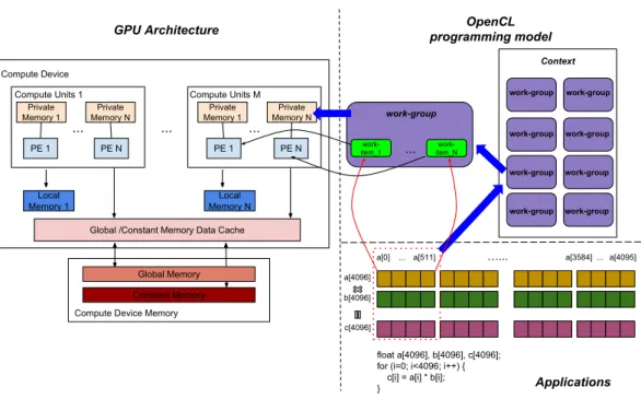
Local and global memories in OpenCL context correspond to the shared and device memories in specified device respectively. As shown in Figure 2.4, each work-group executes on one Compute Unit (CU), each work-item executes on one Process-ing Element (PE). Private memory is assigned to one work-item. Local memory is
... ... ...
work-item_1 ... item_N
work-work-group OpenCL programming model work-group Context GPU Architecture work-group work-group work-group work-group work-group work-group work-group
Global /Constant Memory Data Cache Compute Device Private Memory N Compute Units 1 PE N Private Memory 1 PE 1 Local Memory 1 Private Memory N Compute Units M PE N Private Memory 1 PE 1 Local Memory N Global Memory Constant Memory Compute Device Memory
float a[4096], b[4096], c[4096]; for (i=0; i<4096; i++) { c[i] = a[i] * b[i]; }
a[4096] b[4096] c[4096]
a[0] ... a[511] …... a[3584] ... a[4095]
Applications
Figure 2.4: GPU device architecture and OpenCL programming model shared by all the work-items in the same work-group. Global and constant memory are visible to all work-groups. OpenCL introduces an additional concept which is different with CUDA: Command Queues. Commands launching kernels and access-ing memory are always issued for a specific command queue. A command queue is created on a specific device in a context.
One example of vector multiplication illustrates how the data map on the OpenCL programming model with GPU architecture in Figure 2.4. At first, all the data of array a[4096], b[4096] and c[4096] are stored in the global memory. Then 512 work-items in one work-group load a[0] to a[511], b[0] to b[511] and c[0] to c[511] to local memory before multiplication computation. Each work-item executes c = a×b until all the work-items reach the synchronous point with barrier() function. The left will be the same until the execution complete.
Recently, there are so many programming tools and integrated development en-vironment to use and evaluate OpenCL as illustrated in [13], [14], [15]. Du et al. [13] evaluated OpenCL as a programming tool for developing performance-portable ap-plications for GPGPU They chose triangular solver (TRSM) and matrix multiplica-tion (GEMM) as representative level 3 Basic Linear Algebra Subprograms (BLAS) routines to implement with OpenCL, profiled TRSM to get the time distribution
2.2. OpenCL: An Intermediate Level Programming Model 27
of the OpenCL runtime system, and provided tuned GEMM kernels for both the NVIDIA Tesla C2050 and ATI Radeon 5870. Experimental results described that nearly 50% of peak performance can be obtained in GEMM on both GPUs with OpenCL. Paone et al. [14] presented a methodology to analyze the customization space of an OpenCL application in order to improve performance portability and to support dynamic adaptation. They formulated their case study by implementing an OpenCL image stereo-matching application customized to the STMicroelectron-ics Platform 2012 [16]. They used design space exploration techniques to generate a set of operating points that represent specific configurations of the parameters allowing different trade-offs between performance and accuracy of the algorithm it-self. Jinen et al. [15] described one methodology involved in applying OpenCL as an input language for a design flow of application-specific processors. The key of the methodology is a whole program optimizing compiler that links together the host and kernel codes of the input OpenCL program and parallelizes the result on a customized statically scheduled processor.
Since the programmable GPU make its way to mobile devices, it is interesting to study the new use-cases here. To this end, Leskela et al. [17] of Nokia Corpo-ration created a programming environment based on the embedded profile of the OpenCL standard and verify it against an image processing workload in a mobile device with CPU and GPU back-ends. The early results on performance with CPU + GPU configuration suggested that there is enough room for optimization. Our experimental results based on heterogeneous systems also illustrate the performance enhancement based on the CPU + GPU combination in chapter 3. In the mean-time, more and more portable device start to support OpenCL standard. The Mali OpenCL SDK [18] provides developers a framework and series of samples for devel-oping OpenCL 1.1 application on ARM Mali based platforms such as the Mali-T600 family of GPUs. The samples cover a wide range of use cases that use the Mali GPU to achieve a significant improvement in performance when compared to running on the embedded CPU alone. QUALCOMM also release the Adreno SDK [19] for devel-oping and optimizing OpenCL applications for Snapdragon 400, 600 and 800-based mobile platforms that include the Adreno 300 series GPU and Krait CPUs both.
’s Shared
Figure 2.5: Snapdragon 600 (APQ8064)’s Shared Memory between Host and the Device
In such a SoC platform, CPU and GPU share the same external memory (global memory) which avoids enormous cost of communication and data exchanging like the communication between desktop-level CPU and GPU. It also means that we can fully exploit the potential of OpenCL on heterogonous parallel computing device to address some high computation applications. While the CPU and GPU within Snapdragon have different architecture and performance characteristics, OpenCL provides a programming environment that enables applications to accelerate data parallel computations that leverage both devices.
For example, in the Snapdragon 600 there is a Quad-Core Krait CPU and Adreno 320 GPU. Both the CPU and GPU access to system (host) memory where the input and output data for computations can be stored as shown in Figure 2.5. All calls to OpenCL API functions on the Snapdragon processor are performed on the CPU. The data parallel workloads are written in OpenCL C kernels. The kernels can be built (compiled) to run on either one or both of the Krait CPU and Adreno GPU. In the case of Snapdragon, the application can choose to create command queue(s) for either one or both devices (CPU or GPU). It is up to the application to decide how to partition work so that it can maximally make use of the compute resources of the CPU and GPU devices. Similarly we will discuss about the workload partition and propose our method about workload distribution in the chapter 3.
2.3. The Dataflow Approach: An High Level Programming Model 29
As above description, heterogeneous systems provide new opportunities to in-crease the performance of parallel applications on clusters with CPU and GPU architectures like [20], [21], [22]. Barak et al. [20] presented a package for running OpenMP, C++ and unmodified OpenCL applications on clusters with many GPU devices. Many GPUs Package (MGP) includes an implementation of the OpenCL specifications that allow applications on one hosting-node to transparently utilize cluster-wide devices (CPUs and/or GPUs). MGP provides means for reducing the complexity of programming and running parallel applications on clusters. Herlihy et al. [21] proposed a new methodology for constructing non-blocking and wait free implementations of concurrent objects whose representation and operations are writ-ten as stylized sequential programs with no explicit synchronization. Aoki et al. [22] proposed Hybrid OpenCL, which enables the connection between different OpenCL implementations over the network. Hybrid OpenCL consists of a runtime system that provides the abstraction of different OpenCL implementations and a bridge program that connects multiple OpenCL runtime systems over the network. Hy-brid OpenCL enables the construction of the scalable OpenCL environments which enables applications written in OpenCL to be easily ported to high performance clus-ter compuclus-ters; thus, Hybrid OpenCL can provide more various parallel computing platforms and the progress of utility value of OpenCL applications.
Different with the above OpenCL-based methodologies, our work in this thesis is to generate, to evaluate and to improve OpenCL applications with rapid prototyping methodology. The upper level of this methodology will be detailed in the next section.
2.3 The Dataflow Approach: An High Level
Pro-gramming Model
The complexity introduced by the wide range of hardware architectures makes the optimal implementation of applications difficult to obtain. Moreover the stability of the application has to be early proved in the development stage to ensure the
reliability of the final product. Some tools such as PeaCE [23], SynDEx [24] aim at providing solutions to these problems by automatic steps leading to a reliable prototype in a short time. The aim of rapid prototyping methodologies is from a high-level description of these applications to its real-time implementations on target architecture as automatically as possible.
2.3.1 Definition of reconfigurable video coding
The Reconfigurable Video Coding (RVC) [25] defines a set of standard coding techniques called Functional Units (FUs). FUs form the basis of existing and future video standards, and are standardized as the Video Tool Library (VTL). A FU is described with a portable, platform-independent language called RVC-CAL. Video decoding process is described as a block diagram in RVC, also known as network or configuration, where blocks are the aforementioned FUs. To this end, RVC defines a XML-based format called FU Network Language (FNL) that is used for the de-scription of networks. FNL is another name for the XML Dataflow Format (XDF). A FNL network may declare parameters and variables, has interfaces called ports, where a port is either an input port or an output port, and contains a directed graph whose vertices may be instances of FUs from the VTL or ports.
Figure 2.6 shows an example of the FNL network that represents sobel filter. The block "openImage" indicates the function of load_file, a FU that loads image file, "sobel" indicates the function of sobel_filter, a FU that executes the sobel filter algorithm and "dispImage" indicates the function of display, a FU that shows the final result in the screen. Edges carry data between a source port of the diagram or of an instance to a target port of the diagram or of another instance.
Figure 2.6: Sobel Filter XML Dataflow Format
2.3. The Dataflow Approach: An High Level Programming Model 31
program has several advantages. First of all, it is no longer necessary to define profiles, rather a decoder may use any arbitrary meaningful combination of FUs. Additionally, this allows applications to be reconfigured at runtime by changing the structure of the network that defines the decoding process. This is especially interesting for hardware and memory-constrained devices. Finally, this makes RVC more hardware-friendly because dataflow is a natural way of describing hardware architectures.
2.3.2 Dataflow models of computation
A dataflow Model of Computation (MoC) defines the behavior of a program described as a dataflow graph. A dataflow graph is a directed graph whose ver-tices are actors and edges are unidirectional First-In-First-Out (FIFO) channels with unbounded capacity, connected between ports of actors. The networks of FUs described by the RVC standard are dataflow graphs. Dataflow graphs respect the semantics of Dataflow Process Networks (DPNs) [26], which are related to Kahn Process Networks (KPNs) [27] in the following ways:
1. Those models contain blocks (processes in a KPN, actors in a DPN) that com-municate with each other through unidirectional, unlimited FIFO channels. 2. Writing to a FIFO is non-blocking, i.e. a write returns immediately.
3. Programs that respect one model or the other must be scheduled dynamically in the general case [28].
The main difference between the two models is that DPNs adds non-determinism to the KPN model, without requiring the actor to be non-determinate, by allowing actors to test an input port for the absence or presence of data [26]. Indeed, in a KPN process, reading from a FIFO is blocking: if a process attempts to read data from a FIFO and no data is available, it must wait. Conversely, a DPN actor will only read data from a FIFO if enough data is available, and a read returns immediately. As a consequence, an actor need not be suspended when it cannot read, which in turn means that scheduling a DPN does not require context-switching nor concurrent processes.
32 Chapter 2. Background
❚❤✐s ♠♦❞❡❧ ♣r♦♣♦s❡s t♦ ✐♥❝❧✉❞❡ s♣❡❝✐✜❝ ❛❝t♦r ✐♥ t❤❡ ♠♦❞❡❧✱ ✇❤♦s❡ ♣r♦❞✉❝t✐♦♥✴❝♦♥✲
s✉♠♣t✐♦♥ r❛t❡s ❝❛♥ ❜❡ ❝♦♥tr♦❧❧❡❞ ❜② ❛ ❝♦♥❞✐t✐♦♥❛❧ ✐♥♣✉t t❛❦✐♥❣ ❜♦♦❧❡❛♥ ✈❛❧✉❡s✳ ❚❤❡
❈②❝❧♦✲st❛t✐❝ ❉❛t❛ ❋❧♦✇ ❬
❇❊▲P✾✺
❪ ♠♦❞❡❧ ✭❈❙❉❋✮ ❛❧❧♦✇s t♦ ❞❡s❝r✐❜❡ ♣r♦❞✉❝t✐♦♥✴✲
❝♦♥s✉♠♣t✐♦♥ r❛t❡s ❛s ❛ s❡q✉❡♥❝❡ ♦❢ ✐♥t❡❣❡rs✱ t❤✉s ❛❧❧♦✇✐♥❣ t❤❡ ❛❝t♦r t♦ ❜❡❤❛✈❡ ✐♥ ❛
❞✐✛❡r❡♥t ♠❛♥♥❡r ✐♥ ❛ s❡q✉❡♥❝❡ ♦❢ ❛❝t✐✈❛t✐♦♥s✳ ❚❤❡ P❛r❛♠❡tr✐③❡❞ ❙②♥❝❤r♦♥♦✉s ❉❛t❛
❋❧♦✇ ❬
❇❇✵✶
❪ ✭P❙❉❋✮ ♣♦♣✉❧❛t❡s t❤❡ ✉s❡ ♦❢ ♣❛r❛♠❡t❡rs t❤❛t ❝❛♥ ❛✛❡❝t ♣r♦❞✉❝t✐♦♥✲
s✴❝♦♥s✉♠♣t✐♦♥s r❛t❡s ❛♥❞ ❢✉♥❝t✐♦♥❛❧ ❜❡❤❛✈✐♦r ♦❢ ❛♥ ❛❝t♦r✳ ❙✉❝❤ ♠♦❞❡❧s ♣r♦✈✐❞❡ ❛
❜❡tt❡r ❡①♣r❡ss✐✈❡♥❡ss t❤❛♥ ❙❉❋ ❜✉t ❞❡❝r❡❛s❡s t❤❡ ❛♥❛❧②③❛❜✐❧✐t② ♦❢ t❤❡ ♥❡t✇♦r❦✳ ❚❤❡
❋✐❣✉r❡
✻✳✸
s❤♦✇s ❛ ❝❧❛ss✐✜❝❛t✐♦♥ ♦❢ t❤❡ ❞❛t❛✲✢♦✇ ♠♦❞❡❧s✳ ❲❤✐❧❡ ✐t ✐s ❡❛s② t♦ ❝❧❛ss✐❢②
s♦♠❡ ♠♦❞❡❧s✱ ✐t ✐s ❞✐✣❝✉❧t t♦ ❡st❛❜❧✐s❤ ❛ ❤✐❡r❛r❝❤② ❜❡t✇❡❡♥ s♦♠❡ ♦❢ t❤❡♠✳ ❋♦r ❡①✲
❛♠♣❧❡ P❙❉❋✱ ❈❙❉❋ ❛♥❞ ❇❉❋ r❡❛❧❧② s❤♦✇ ❞✐✛❡r❡♥t ❜❡❤❛✈✐♦r ❛♥❞ t❤❡ ❝❧❛ss✐✜❝❛t✐♦♥
❡st❛❜❧✐s❤❡❞ ✐♥ ❋✐❣✉r❡
✻✳✸
✐s ♥♦t r❡❧❡✈❛♥t✳
KPN DPN PSDF PSDF CSDF BDF SDF HSDF DAG ExpressivenessKPN: Kahn Process Network DPN: Dala-flow Process Network
PSDF: Parametrized Synchronous Data Flow CSDF: Cyclo-static Synchronous Data Flow BDF: Boolean-controlled Data Flow SDF: Synchronous Data Flow
HSDF: Homogeneous Synchronous Data Flow DAG: Directed Acyclic Graph
Analyzability ❋✐❣✉r❡ ✻✳✸✿ ❉❛t❛✲✢♦✇ ▼♦❞❡❧s ♦❢ ❝♦♠♣✉t❛t✐♦♥ t❛①♦♥♦♠②✳
■♥ t❤❡ ❢♦❧❧♦✇✐♥❣ ✇❡ ✇✐❧❧ ❣✐✈❡ ❛♥ ✐♥tr♦❞✉❝t✐♦♥ t♦ t❤❡ ❞❛t❛✲✢♦✇ ♣❛r❛❞✐❣♠ st❛rt✐♥❣
❜② t❤❡ ♠♦t❤❡r ♦❢ ❛❧❧✱ t❤❡ ❑❛❤♥ Pr♦❝❡ss ◆❡t✇♦r❦ ❢♦❧❧♦✇❡❞ ❜② t❤❡ ❉❛t❛ ❋❧♦✇ Pr♦❝❡ss
◆❡t✇♦r❦ ❛♥❞ ♣r♦✈✐❞❡ ❛♥ ✐♥✲❞❡♣t❤ ❡①♣❧♦r❛t✐♦♥ ♦❢ t❤❡ ♣r❡✈✐♦✉s❧② ❝✐t❡❞ ♠♦❞❡❧s✳
✻✳✸✳✷ ❉❛t❛ ❋❧♦✇ ♣❛r❛❞✐❣♠ ✐♥tr♦❞✉❝t✐♦♥
❑❛❤♥ Pr♦❝❡ss ◆❡t✇♦r❦ ✭❑P◆✮
❆ ♣r♦❝❡ss ♥❡t✇♦r❦ ✐s ❛ s❡t ♦❢ ❝♦♥❝✉rr❡♥t ♣r♦❝❡ss❡s t❤❛t ❛r❡ ❝♦♥♥❡❝t❡❞ t❤r♦✉❣❤
♦♥❡✲✇❛② ✉♥❜♦✉♥❞❡❞ ❋■❋❖ ❝❤❛♥♥❡❧s✳ ❊❛❝❤ ❝❤❛♥♥❡❧ ❝❛rr✐❡s ❛ ♣♦ss✐❜❧② ✜♥✐t❡ s❡q✉❡♥❝❡
✭❛ str❡❛♠✮ t❤❛t ✇❡ ❞❡♥♦t❡
✳ ❊❛❝❤
✐s ❛♥ ❛t♦♠✐❝ ❞❛t❛ ♦❜❥❡❝t ❝❛❧❧❡❞
t♦❦❡♥ ❜❡❧♦♥❣✐♥❣ t♦ ❛ s❡t✳ ❚♦❦❡♥ ❝❛♥♥♦t ❜❡ s❤❛r❡❞✱ t❤✉s t♦❦❡♥s ❛r❡ ✇r✐tt❡♥ ✭♣r♦✲
❞✉❝❡❞✮ ❡①❛❝t❧② ♦♥❝❡ ❛♥❞ r❡❛❞ ✭❝♦♥s✉♠❡❞✮ ❡①❛❝t❧② ♦♥❝❡✳ ❆s ❋■❋❖s ❛r❡ ❝♦♥s✐❞❡r❡❞
Figure 2.7: Data-flow Models of Computation (MoC) taxonomy
The CAL dataflow programming model is based on the DPN model, where an actor may include multiple firing rules. Many variants of dataflow models have been introduced in Figure 2.7: Data-flow MoC taxonomy. RVC-CAL is expressive enough to specify a wide range of programs that follow a variety of dataflow models. A CAL dataflow program can fit into those models depending on the environment and the target application.
Dataflow process network model
Each FIFO channel is a DPN carries a sequence of tokens X = [x1, x2...], where
each xi is called a token. The sequence of available tokens on the Pth input port is
Xp. An empty FIFO ⊥ corresponds to the empty sequence. If a sequence X belong
another sequence Y , for example X = [1, 2, 3, 4], Y = [1, 2, 3, 4, 5, 6], we can define that X ⊑ Y .
The set of all possible sequences is defined as S, and Sp is the set of p-tuples of
sequence. In other words [X1, X2, ..., XP] ∈ Sp.
An actor executes or fires when at least one of its firing rules is satisfied. Each firing consumes and produces tokens. An actor has N firing rules:
2.3. The Dataflow Approach: An High Level Programming Model 33
A firing rule Ri is a finite sequence of patterns, one for each of the p input ports of
the actor:
Ri = [Pi,1, Pi,2, ..., Pi,p] ∈ Sp (2.2)
A pattern rule Pi,j defines an acceptable sequence of tokens: if Pi,j ⊑ Xj, the
pattern is satisfied for the sequence of unconsumed (or available) tokens on the pth
input port; if Pi,j =⊥, the pattern is satisfied for any sequence, which is different
from Pi,j = [∗] that defines a pattern satisfied for any sequence containing at least
one token.
Synchronous dataflow model
The Synchronous Dataflow (SDF) [29] model is one of the most studied in our applications. SDF is the least expressive DPN model, but it is also the model that can be analyzed more easily. The SDF model is a special case of DPN where actors have static firing rules. They consume and produce a fixed number of tokens each time they fire. Any two firing rules Ra and Rb of an SDF actor must consume the
same amount of tokens:
|Ra|= |Rb| (2.3)
SDF may be easily specified in CAL constraining actions to have the same token consumption and production. Moreover, production and consumption rates may be easily extracted from an actor to check the SDF properties of actors at compile time. A key feature of this model is that a static code analysis detects if the program can be scheduled at compile time. A static analysis produces a static schedule (a predefined sequence of actor firings), if it exists, which is free of deadlock and that uses bounded memory.
Cyclo-static Dataflow (CSDF) [30] extends SDF with the notion of state while retaining the same compile-time properties concerning scheduling and memory con-sumption. State can be represented as an additional argument to the firing rules and firing function, in other words it is modeled as a self-loop. The position of the state argument (if any) is the first argument of a firing rule, i.e. it comes before patterns. The equations defined in the previous section for SDF can be naturally extended to
express the same restrictions (fixed production/consumption rates) for each possible state of the actor. Like SDF, CSDF graphs can be scheduled at compile-time with bounded memory. Our dataflow approach of SigmaC is based on CSDF model.
Parameterized SDF (PSDF) which was introduced in [31] that is a special case of SDF. This model aims at increasing SDF expressiveness while maintaining its com-pile time predictability properties. In this model a sub-system (sub-graph) behavior can be controlled by a set of parameters that can be configured dynamically. These parameters can either configure sub-system interface behavior by modifying produc-tion/consumption rate on interfaces, or configure behavior by passing parameters (values) to the sub-system actors.
2.3.3 Dataflow sigmaC
To exploit the parallelism available in the platform MPPA, Kalray has developed its own dataflow model: SigmaC. According to this model, the block in dataflow graph is called agent. Each agent is appointed and includes: the C code of the function executed, the number of incoming and outgoing data through the interface together with the set of production/consumption. All these information are assigned through a special syntax, specific SigmaC that illustrated as Figure 2.8.
Every agent define that it remains only to create the graph by interacting. To do this, a new syntax is created in order to create graph and sub-graph and thus to organize the work as cleanly as possible. Figure 2.9 illustrates the example of sub-graph syntax connecting two agents.
2.3.4 RVC-CAL language
This part presents the RVC-CAL language and covers the syntax, semantics with this kind of language. RVC-CAL is a Domain-Specific Language (DSL) that has been standardized by RVC as a restricted version of CAL. CAL was invented by Eker and Janneck and is described in their technical report [1].
2.3. The Dataflow Approach: An High Level Programming Model 35
Figure 2.8: SigmaC: syntax of one agent
Figure 2.9: SigmaC: syntax of subgraph with two agents a1 et a2
Actor structure
An RVC-CAL actor is an entity that is conceptually separated into an header and a body. The header describes the name, parameters, and port signature of the actor. For instance, the header of the actor shown in the Figure 2.10 defines an actor called select. This actor takes two parameters, one boolean and one integer, whose values are specified at runtime, when the actor is instantiated, i.e. when it is initialized by the network that references it. The port signature of select is an input port Cost and one output ports Disp. The body of one actor may be empty, or contains state variables declarations, functions, procedures, actions, priorities, and at most one Finite State Machine (FSM).
actor select(bool checkHeaderCRC, int accetpedMethods)
float Cost ==> float Disp:
//body
end
Figure 2.10: The header of an RVC-CAL Actor of those steps:
1. the actor may consume tokens from its input ports, 2. it may modify its internal state,
3. it may produce tokens at its output ports.
Consequently, describing an actor involves describing its interface to the outside, the ports, the structure of its internal state, as well as the steps it can perform, what these steps do (in terms of token production and consumption, and the update of the actor state), and how to pick the step that the actor will perform next.
State variables
State variables can be used to define constants and to store the state of the actor. Figure 2.11 shows the three different ways of declaring a state variable. The
uint(size=16) Number = 0x1fff;
// the bits of the byte read
uint(size=16) bits;
// number of bits remaining in value
uint(size=4) num_bits := 32;
Figure 2.11: Declaration of State Variable
first variable Number is a 16-bit unsigned integer constant. The bits variable is a 16-bit unsigned integer variable without an initial value. The num_bits variable is a 4-bit unsigned integer that is initialized to 32. The difference between the = used
2.3. The Dataflow Approach: An High Level Programming Model 37
to initialize a constant and the := used to initialize a variable. The initial value of a variable is an expression.
Function
As shown in Figure 2.12, a function may declare parameters such as n of bit_-number and local variables, like eof. The body of a function is an expression whose type must match the specified type of the function.
function bit_number(int n ) --> bool var
bool eof = get_eof_flag();
if eof then false else num_bits >= n end end
Figure 2.12: Declaration of a Function
Actions
So far, the only firing condition for actions was that there be sufficiently many tokens for them to consume, as specified in their input patterns. However, in many cases we want to specify additional criteria that need to be satisfied for an action to fire conditions, for instance, that depend on the values of the tokens, or the state of the actor, or both. These conditions can be specified using guards, as for example in the Split actor in Figure 2.13: An action may have firing conditions, called guards,
actor Split () Input ==> P, N:
action [a] ==> P: [a] guard a >= 0 end
action [a] ==> N: [a] guard a < 0 end
end
Figure 2.13: Declaration of a Action
where the action firing depends on the values of input tokens or the current state. Guards are included in scheduling information that defines the criteria for action to fire. The contents of an action, that are not scheduling information, are called its
body, and define what the action does. The difference is not so clear, for instance the expressions in the output pattern are part of the body, but the output pattern itself is scheduling information as it holds the number of tokens produced by the action. When an actor fires, an action has to be selected based on the number and values of tokens available and whether its guards are true. Action selection may be further constrained using a FSM, to select actions according to the current state, and priority inequalities, to impose a partial order among action tags.
Finite state machine (FSM)
An FSM is defined by the triple where S is the set of states, is the initial state, and is the state-transition function: Note that a state transition allows a set of actions to be fireable. Figure 2.14 presents an example of a simple actor that downsamples its input stream by two.
actor Downsample() bool R ==> bool R2: a0 : action R:[r] ==> end a1 : action R:[r] ==> R2:[r] end schedule fsm s0: s0 (a0) --> s1; s1 (a1) --> s0; end end
Figure 2.14: A simple actor with an FSM
2.4 Tools of Rapid Prototyping Methodology
This section presents some tools integrated in our rapid prototyping methodology such as Orcc, Preesm, and HMPP.
2.4. Tools of Rapid Prototyping Methodology 39
2.4.1 Orcc, an Open RVC-CAL Compiler
Orcc include an RVC-CAL textual editor, a compilation infrastructure, a simu-lator and a debugger [2]. The primary purpose of Orcc is to provide developers with a compiler infrastructure to allow several languages and combination of languages (in the case of co-design) to be generated from RVC-CAL actors and networks. Orcc does not generate assembly or executable code directly; rather it generates source code that must be compiled by another tool. This tool can generate code for any platform, including hardware (VHDL), software (C/C++, Java, LLVM...), and heterogeneous platforms (mixed hardware/software) from a RVC-CAL description.
How we could obtain the target code for specified architecture from the RVC-CAL description of our applications. This is the procedure of compilation. This section describes basic concepts of compilation, and in particular the concepts that are necessary to understand our work as described in the next chapters. Compilation is the process by which a program in a source language is transformed to another semantically-equivalent program in a target language as shown in Figure 2.15.
front-end middle-end back-end RVC-CAL actors actorsIR source code IR actors XDF networks XDF networks
Figure 2.15: Compilation procedure of Orcc
The first stage of the compiler, called front-end, is responsible for creating an Intermediate Representation (IR) of RVC-CAL actors, the resulting actors being called IR actors. The middle-end is the component that analyzes and transforms the IR of actors and networks to produce optimized IR actors and networks. The last stage of the compiler is code generation, in which the back-end for a given language (C, LLVM, VHDL, etc) generates code from a hierarchical network and a set of IR
actors.
2.4.2 Preesm, a Parallel and Real-time Embedded
Execu-tives Scheduling Method
The PREESM tool offers a fast prototyping tool for parallel implementations [3]. The inputs of the tool are architecture and algorithm graphs and a scenario that basi-cally gathers all information linking algorithm and architecture. The target architec-tures are embedded heterogeneous architecarchitec-tures, with possibly several processors and many cores. The current version of PREESM focuses on static mapping/scheduling of algorithms. The Model of Computation (MoC) is used to describe algorithms based on Synchronous Dataflow Graphs (SDF) extended with the hierarchy feature. The PREESM tool is not suitable for adaptable applications (DPN MoC of Orcc) in which the mapping/scheduling should be done partially or completely at runtime.
2.4.3 HMPP, a Hybrid Multicore Parallel Programming model
HMPP developed by CAPS, is a directive-based compiler to build parallel GPU applications, and support for the OpenACC standard [4]. HMPP offers a high level abstraction for hybrid programming that fully leverages the computing power of stream processors with a simple programming model. HMPP compiler integrates powerful data-parallel backends for NVIDIA CUDA and OpenCL that drastically reduce development time. The HMPP runtime ensures application deployment on multi-GPU systems. Software assets are kept independent from both hardware plat-forms and commercial software. While preserving portability and hardware interop-erability, HMPP increases application performance and development productivity.
These are two basic paired directives of HMPP: Codelet and Callsite. Codelet is used before the definition of C functions. Callsite is the HMPP directive for invocation on such an accelerator device. Using only simple paired directives, HMPP can replace the complex procedure of manually writing the CUDA/OpenCL kernel code. For the basic HMPP’s transformation, we just need to insert two lines of directives into the source C code as shown in Algorithm 1:
2.4. Tools of Rapid Prototyping Methodology 41
Algorithm 1: HMPP_Transformation()
1 #pragma hmpp motion_estimation codelet, target=CUDA; 2 Definition of function motion_estimation();
3 ...;
4 Main(argc, argv);
5 #pragma hmpp motion_estimation callsite; 6 Function call of motion_estimation();
For exploiting the better performance with HMPP, hmppcg directives can opti-mize the performance of generated HMPP kernel code:
1. The hmppcg gridify directives determine which loop should be parallelized. Because of the gridify(i, j), the i and j for-loops in line 3 and 4 will be parallelized.
1 # pragma hmppcg g r i d i f y (j , i ) 2 for( k = 0; k < N ; k ++) 3 for( j = 0; j < H ; j ++) 4 for ( i = 0; i < W ; i ++){ 5 ... 6 }
2. The hmppcg grid allocate the buffer (data storage region in device) to shared memory. The specified buffer will be loaded into shared memory before complex computations. Because accessing the shared memory is faster than the global mem-ory (more details will be discussed in the 3.1), time efficiency will benefit from the hmppcg grid directive.
1 # pragma hmppcg grid shared buffer
3. Level 1 cache, is a static memory integrated with processor core that is used to store information recently accessed by a processor. Level 1 cache is often abbreviated as L1 cache. The purpose of L1 cache is to improve data access speed in cases when the processor accesses the same data multiple times. In NVIDIA’s GPU devices of compute capability 2.0 and later, there is 64 KB of memory for each multiprocessor. This per-multiprocessor on-chip memory is split and used for both shared memory and L1 cache. By default, 48 KB is used as shared memory and 16 KB as L1 cache. The configuration of L1 cache preference: there is an obvious improvement of performance in our experiments.
Original algorithms with
C/C++/FORTRAN Sequential computing
HMPP Compiler
HMPP to OpenCL/CUDA
code computingParallel
Manual CUDA/OpenCL
GPU CPU
CPU
If source code changes, no more work for user
If source code change, lot of modifications are
applied by user.
FPGA
Figure 2.16: HMPP workflow in COMPA project
1 c u d a D e v i c e S e t C a c h e C o n f i g ( args );
2 args = c u d a F u n c C a c h e P r e f e r L 1 ;
Based on hmppcg directives, we can obtain great performance enhancement com-paring with default HMPP. The HMPP backend of Orcc will seek out the part of parallelism in original C code like multi-level for loops, and insert the HMPP direc-tives into suitable position of C code. When we compile the C code with HMPP directives, we can obtain the .cu or .cl file for the execution of full search function which targets to GPU. Furthermore, as shown in Figure 2.16, we only need to main-tain and modify the C source code, and HMPP will produce the CUDA/OpenCL kernels according to the source C code of applications.
2.5 Concerned Image and Video Processing
Al-gorithms
Video decoders with Orcc and Preesm used to evaluate the prototyping frame-work in the previous research frame-work. But video decoders are usually based on the dataflow and structure with a lot of data dependencies which are very hard to map
2.5. Concerned Image and Video Processing Algorithms 43
with parallelism and to implement on many core heterogeneous systems. Some parallel applications are proposed in this thesis to evaluate the rapid prototyping framework which can fully make use of the parallelism of target architectures. Thus they are suitable to evaluate the efficiency of the rapid prototyping framework.
2.5.1 Motion estimation
Motion estimation (ME) is the process of determining motion vectors that de-scribe the transformation from one 2D image to another, usually from adjacent frames in a video sequence. It is an ill-posed problem as the motion is in three dimensions but the images are a projection of the 3D scene onto a 2D plane. ME is the main time-consuming task of a video encoder with more than half of the whole computation load. In order to eliminate temporal redundancy, ME could find relative motions between two images as shown in Figure 2.17. The motion vectors
Figure 2.17: Motion estimation illustration
may relate to the whole image (global motion estimation) or specific parts, such as rectangular blocks, arbitrary shaped patches or even per pixel. The motion vec-tors may be represented by a translational model or many other models that can approximate the motion of a real video camera, such as rotation and translation in all three dimensions and zoom. Closely related to motion estimation is optical flow, where the vectors correspond to the perceived movement of pixels. Applying the motion vectors to an image to synthesize the transformation to the next image
is called motion compensation. The combination of motion estimation and motion compensation is a key part of video compression standard as used by H.264 and HEVC as well as many other video codecs.
The methods of motion estimation can be categorized into pixel based direct methods and feature based indirect methods.
Direct Methods
– Block-matching algorithm [32]
– Phase correlation and frequency domain algorithms [33] – Pixel recursive algorithms [34]
– Optical flow algorithms [35]
Indirect Methods employs features, such as corner detection, and match corre-sponding features between frames, usually with a statistical function applied over a local or global area. The purpose of the statistical function is to remove matches that do not correspond to the actual motion.
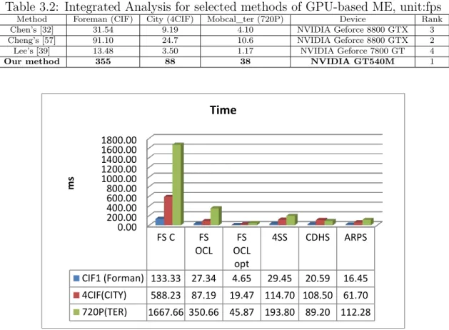
Block matching ME algorithms are most widely used in video compression stan-dard, also the most concerned in this thesis. There is a brief overview of available motion estimation systems shown in Table 2.2. The frames per second (fps) indi-cates the processing speed of the different systems.
Table 2.2: Overview of Motion Estimation implementations
References Algorithms Resolution and search region fps Platform
mehta et al. [36] threshold in the SAD 640 × 480, 32 × 32 52.5 GPU martin et al. [37] samll diamond search 352 × 288, 16 × 16 20 GPU chen et al. [32] variable block size 352 × 288, 32 × 32 31.5 GPU Luo et al. [38] content adaptive search technique 352 × 288, 32 × 32 60.7 CPU Lee et al. [39] multi-pass full search 352 × 288, 32 × 32 8.89 GPU Li et al. [40] most significant bit 640 × 480, 32 × 32 129 FPGA Urban et al. [41] HDS for Hierarchical Diamond Search 720 × 576, 32 × 32 100 DSP
2.5.2 Stereo matching
As shown in Figure 2.18, stereo matching is a technique aimed at computing depth information from two cameras used in many applications such as 3D-TV, 3D reconstruction and 3D object tracking.
2.5. Concerned Image and Video Processing Algorithms 45
Figure 2.18: Overview of the view stereo matching process, where (a) the stereo vision is captured in a left and right image, (b) the disparities are searched through stereo matching.
P OR OT p1 p2 B (baseline) XR X T f
Figure 2.19: Basic concepts of stereo matching in epipolar geometry
Figure 2.19. The object point P corresponds to the pixel p1 from the left frame and the pixel p2 from the right frame. OT is the target optical center (left camera)
and ORis the reference optical center (right camera). The distance between the two
optical centers is defined as the Baseline represented by B, which is parallel with by epipolar lines, and the length f from frame plane to B is the focal distance. In the case shown in Figure 2.19, the distance from P to B is defined as the depth Z which is the actual distance between cameras and object point, and the distance from p1 to p2 is defined as the disparity d = XT − XR), which is the displacement
of one stereo pair’s locations in the stereo frames. Considering the similar triangles (P OROT and P p1p2), we obtain the relationship between depth Z and disparity d:
B Z = (B + XR) − XT Z − f ⇒ Z = B · f XT − XR = B · f d (2.4)
The above equation basically demonstrates that the more deep the object lies, the less disparity it has between the stereo pair in the input videos, and this principle is also the basis of stereo matching. Figure 2.20 elaborates the stereo matching technique with two rectified images from middlebury stereo database [42]. Figure 2.21 lists the histogram of matching cost value, the max bin in this histogram means the best matching result.