RESEARCH OUTPUTS / RÉSULTATS DE RECHERCHE
Author(s) - Auteur(s) :
Publication date - Date de publication :
Permanent link - Permalien :
Rights / License - Licence de droit d’auteur :
Bibliothèque Universitaire Moretus Plantin
Institutional Repository - Research Portal
Dépôt Institutionnel - Portail de la Recherche
researchportal.unamur.be
University of Namur
Theory of Turing Patterns on Time Varying Networks
Petit, Julien; Lauwens, Ben; Fanelli, Duccio; Carletti, Timoteo
Published in:
Physical review letters
DOI:
10.1103/PhysRevLett.119.148301
Publication date:
2017
Document Version
Peer reviewed version
Link to publication
Citation for pulished version (HARVARD):
Petit, J, Lauwens, B, Fanelli, D & Carletti, T 2017, 'Theory of Turing Patterns on Time Varying Networks',
Physical review letters, vol. 119, no. 14, 148301, pp. 148301-1 148301-5.
https://doi.org/10.1103/PhysRevLett.119.148301
General rights
Copyright and moral rights for the publications made accessible in the public portal are retained by the authors and/or other copyright owners and it is a condition of accessing publications that users recognise and abide by the legal requirements associated with these rights. • Users may download and print one copy of any publication from the public portal for the purpose of private study or research. • You may not further distribute the material or use it for any profit-making activity or commercial gain
• You may freely distribute the URL identifying the publication in the public portal ?
Take down policy
If you believe that this document breaches copyright please contact us providing details, and we will remove access to the work immediately and investigate your claim.
The theory of Turing patterns on time varying networks
Julien Petit1,2, Ben Lauwens2, Duccio Fanelli3,4, Timoteo Carletti1
1naXys, Namur Institute for Complex Systems,
University of Namur, Belgium
2Department of Mathematics,
Royal Military Academy, Belgium
3Dipartimento di Fisica e Astronomia and CSDC,
Universit`a degli Studi di Firenze, Italy
4INFN Sezione di Firenze, Italy
The process of pattern formation for a multi-species model anchored on a time varying network is studied. A non homogeneous perturbation superposed to an homogeneous stable fixed point can amplify, following the Turing mechanism of instability, solely instigated by the network dynamics. By properly tuning the frequency of the imposed network evolution, one can make the examined system behave as its averaged counterpart, over a finite time window. This is the key observation to derive a closed analytical prediction for the onset of the instability in the time dependent framework. Continuously and piecewise constant periodic time varying networks will be analysed, to set the ground for the proposed approach. The extension to non periodic settings will also be discussed.
Spatially extended systems can spontaneously yield a multitude of patterns, resulting from an inherent drive to self-organization [1–3]. In many cases of interest, the interplay between nonlinearities and di↵usion seeds a symmetry breaking instability (discovered by Turing in his pioneering work on morphogenesis). This insta-bility paves the way to the emergence of a rich gallery of patchy motifs [4–6]. Distinct populations of homolo-gous constituents often interact via an intricate architec-ture of nested couplings, which can be adequately rep-resented as complex heterogeneous networks. Elaborat-ing on the mechanisms that instigate pattern formation for reaction-di↵usion systems hosted on small lattices or large complex networks is hence central to diverse phe-nomena of broad applied and fundamental impact [7–12]. Topology is known to play, in this respect, a role of paramount importance. Illustrative are oscillatory pat-terns [13, 14] that can rise only if the support is directed. Further, self-organisation may proceed across multiple, interlinked networks, by exploiting assorted resources and organisational skills. Multiplex networks have been therefore introduced as a necessary leap forward in the modeling e↵ort: these are particularly relevant to trans-portation systems, the learning organisation in the brain and to understanding the emergent dynamics in social communities. Interestingly, the interaction between ad-jacent layers can yield self-organised patterns which are instead impeded in the limit of decoupled layers [16, 17]. Patterns on individual layers can also fade away due to cross-talking between contiguous slabs. All these exam-ples, point to the pivotal role exerted by the topology of the underlying network in shaping macroscopic behavior of the system [15].
In several realms of application, the networks that specify the routing of the spatial or physical interactions are not static, but, instead, do evolve in time [18–21]. This is an important additional ingredient key to
im-prove on our current understanding of the mechanisms responsible for the appearance of structured patterns across heterogenous networks. In the framework of tem-poral networks, di↵usion processes [22] as well as random walks [23, 24] have been studied in recent years, mostly under the assumption of piecewise constant time varying networks [25–27]: the topology of the assigned connec-tions is fixed over a finite window in time, whose dura-tion can either depend on the dynamics of the system or be exogenously controlled. The couplings are then in-stantaneously created, destroyed or rewired, at the end of each time window, and the ensuing network frozen for the subsequent time interval . Prototypical examples are contact networks [28, 29]. Synchronisation phenomena have also been considered for nonlinear oscillators [30] hosted on time varying networks, as well as for systems displaying generic reactions terms [25, 31, 32].
In this Letter we consider for the first time the pro-cess of pattern formation for reaction-di↵usion systems anchored on networks that evolve over time. To this end, we initially inspect the case of a network that is periodically rearranged in time. In particular we prove that a symmetry breaking instability which anticipates the pattern derive can be incited, by properly tuning the frequency of the imposed network dynamics. The proposed framework includes the case of a continuously time varying network (links weights change as a smooth function of time) and the one where sudden switches be-tween distinct discrete networks configurations are to be accounted for. Surprisingly enough, patterns can emerge for a reaction-di↵usion system hosted on a piecewise con-stant time varying network, also when they are formally impeded on each network snapshot. The extension to non periodic settings will be also analysed, allowing us to draw a general interpretative scenario. Local dynam-ics is slower than the typical time scales implicated in the network rearrangements, for the sought e↵ects to
man-ifest. This setting is e.g. relevant for modeling virus spreading as mediated by pairwise contacts.
Imagine two di↵erent species living on a network that evolves over time and denote by uiand vitheir respective
concentrations, as seen on node i. Links can change their (positive) weights, they can fade away (the corresponding weight goes to 0), or be created (a null weight is turned positive) or even rewired (a combination of both preced-ing moves). For the sake of simplicity, and without lospreced-ing generality, we assume constant the number of nodes N . The network structure is stored in a time varying N⇥ N weighted adjacency matrix, Aij(t). The strength si(t) of
node i is computed as si(t) = PjAij(t). Species can
relocate in space, as follows a standard di↵usive mecha-nism, ruled by the (time dependent) Laplacian operator Lij(t) = Aij(t) si(t) ij. Remark that, for all t and all
i,PjLij(t) = 0, namely L(t) is a row stochastic matrix.
When species happen to share the same node, they mu-tually interact via nonlinear terms that reflect the speci-ficity of the problem at hand. We will deal at first with networks that are periodically reset in time, and show how adjusting the period of the modulation can trigger the onset of patterns.
The model can be mathematically cast in the form: ˙ui(t) = f (ui, vi) + Du N X j=1 Lij(t/✏)uj(t) ˙vi(t) = g(ui, vi) + Dv N X j=1 Lij(t/✏)vj(t) (1)
where f and g stand for the generic nonlinear reactions terms and Du and Dv label the di↵usion coefficients of
species u and v, respectively. The parameter ✏ controls the period of the Laplacian oscillations in time. We will in particular denote with T the period obtained for ✏ = 1. When the oscillations materialise as successive swaps be-tween two (or more) network configurations, it is the fre-quency of the blinking that sets the patterns derive, also when Turing motifs cannot manifest for the model con-strained on any of the considered (static) network snap-shots. As a further preliminary condition we assume that system (1) admits an homogeneous stable fixed point. In other words, there exists (ui, vi) = (¯u, ¯v) such that
˙ui= ˙vi= 0, for all i = 1, . . . , N .
Define the averaged LaplacianhLi = T1 R0TL(t)dt and introduce the averaged reaction-di↵usion system:
˙ui(t) = f (ui, vi) + Du N X j=1 hLijiuj ˙vi(t) = g(ui, vi) + Dv N X j=1 hLijivj, (2)
Our main result goes as follows : assume system (2) satisfies the conditions for the emergence of Turing pat-terns, namely an external non homogeneous perturbation
triggers the instability of the homogeneous fixed point (¯u, ¯v). Then, ✏⇤ > 0 exists such that system (1) also
undergoes Turing instabilities for 0 < ✏ < ✏⇤.
Here, 1/✏⇤ acts as an e↵ective high frequency drive
for self-organised spatial motifs to develop. The idea of the proof is sketched in the following, further details are relegated in the Supplementary Information (SI), where the result is presented in the form of a theorem.
Label ⌧ = t/✏ and introduce the com-pact notation ~x = (u1, . . . , uN, v1, . . . , vN).
Then define the function F by F (~x) = (f (u1, v1), . . . , f (uN, vN), g(u1, v1), . . . , g(uN, vN)),
the block matrix L(t) := ⇣DuL(t) 0
0 DvL(t) ⌘
, and the corresponding time average hLi. Then, by virtue of the theorem of averaging one can show that there exists ✏⇤ > 0 such that for all 0 < ✏ < ✏⇤ and ⌧ =O(1/✏), one
has ~x(⌧ ) ~y(⌧ ) =O(✏), where ~x(⌧) is the solution of ~x0(⌧ ) = ✏ [F (~x) +L(⌧)~x] , ~x(0) = ~x02 R2N, (3)
where the prime denotes the derivative with respect to the rescaled time ⌧ and ~y(⌧ ) is the solution of the associ-ated average system ~y0(⌧ ) = ✏ [F (~y) +hLi~y], subject to the same initial conditions, ~y(0) = ~x0. Since the reaction
term is time independent, the average solely a↵ects the di↵usive part.
Back to the original variables, the solutions of, respec-tively, the time dependent system (with ✏2 (0, ✏⇤]) and
the averaged one, stay close for times O(1). Hence, if an injected perturbation destabilises the homogenous so-lution of (2), the same holds when the perturbation is applied to system (1). Remark however that the two sys-tems behave similarly, only for a finite time span. In fact there is no e↵ective or exponential stability `a la Nekhoro-shev. Stated di↵erently, we cannot guarantee that the smaller ✏ the longer the two systems agree. This in turn implies that the asymptotic patterns, which follows the initial instability and as obtained for respectively the av-eraged and the time dependent models, may, in principle, di↵er. We will return later on characterising the critical threshold ✏⇤.
We will hereafter discuss a pedagogical application (termed the twin networks case) aimed at clarifying the conclusion reached above. Other examples, to which we will allude in the following, are instead presented in the SI. Begin by considering the Brusselator model, a widely studied model of chemical oscillators. This choice amounts to setting f (u, v) = 1 (b + 1)u + cu2v and
g(u, v) = bu cu2v where b, c stand as free parame-ters. When the model is made spatially extended, the coaction of di↵usion and reaction terms can disrupt the homogeneous fixed point, paving the way to the patterns outbreak. This occurs when the parameters are set so as to make the dispersion relation (max< , the real part of the complex exponential growth rate ) positive over a finite window of wave-numbers. When the di↵usion takes
3 place on a heterogeneous network, the dispersion relation
is defined on a discrete support that coincides with the eigenvalues of the Laplacian operator. If the spectrum of the discrete Laplacian operator falls in a region where the continuous dispersion relation is negative, no instability can take place on the network, even if it can develop on a continuum support. This observation will be central for what follows.
Let us thus consider two simple networks, made of N nodes arranged on a periodic ring, and label with A1and
A2 their respective adjacency matrices. The (even) N
nodes are connected in couples, the twins, via symmetric links. In the first case (the network that is encoded in A1) nodes 2k 1 and 2k, for k = 1, . . . , N/2 are tight
together. In the other, the couples are formed by nodes (2k, 2k + 1) for k = 1, . . . , N/2 1, with the addition of pair (N, 1) (see Fig. 1 panel a). Both networks yield an identical Laplacian spectrum: two degenerate eigenvalues are found, ⇤1= 0, with multiplicity N/2 (i.e. the number
of connected components the network is made of) and ⇤N = 2, with multiplicity N/2. The parameters are
set so that patterns cannot emerge for the Bussellator model defined on each of the networks introduced above. This is shown in Fig. 1 panel c.
We now introduce a periodically time varying network, specified by the following adjacency matrix A(t):
A(t) = (
A1 if{t/T } 2 [0, )
A2 if{t/T } 2 [ , 1) ,
(4)
where{r} denotes the fractional part of the real number r and 2 (0, 1) is the fraction of occurrence of the first network (and thus 1 for the second one) during the period T > 0. The Laplacian matrix L(t) can be com-puted accordingly. We get the averaged Laplacian matrix hLi = L1+ (1 )L2where Liis the Laplacian matrix
of the i–th network, i = 1, 2. As an example, assume = 0.3, T = 1 and compute the dispersion relation asso-ciated to the averaged networkhAi = A1+ (1 )A2.
From inspection of Fig. 1 panel c), it is immediately clear that ⇤↵, the eigenvalues of the Laplacian
hLi, fall in a region where< ↵> 0. Hence, the Brusselator placed on
the average network exhibits Turing patterns (see Fig. 1 panel d). Based on the above, we can find a positive ✏⇤ such that for all 0 < ✏ < ✏⇤the time dependent system (1) displays patterns. This is because this latter system is close enough to the averaged counterpart to be able to follow its orbits. On the other hand, no patterns can develop if ✏ is too large. These conclusions are clearly demonstrated in Fig. 2 panel a).
We now complement the analysis by elaborating on a recipe to estimate the critical threshold ✏⇤. Assume ✏ = 1
and linearise system (1) close to the stable homogeneous equilibrium (ui, vi) = (¯u, ¯v), for all i = 1, . . . , N :
d ~x
dt = M(t) ~x , (5)
where ~x = (u1 u, . . . , u¯ N u, v¯ 1 v, . . . , v¯ N v)¯ T and
M(t) = @xF (¯u, ¯v)+L(t), where @xF (¯u, ¯v) is the Jacobian
of the reaction part evaluated at the homogeneous equi-librium. M(t) is T -periodic and piecewise constant, more precisely M(t) = @xF (¯u, ¯v) +L1:= M1if{t/T } 2 [0, )
and M(t) = @xF (¯u, ¯v) +L2 := M2 if {t/T } 2 [ , 1).
We can thus solve exactly Eq. (5) over one period yield-ing ~x(T ) = eM2(1 )TeM1 T ~x(0) =: Q ~x(0) where the rightmost equality defines the monodromy matrix, Q. Hence, for any m 1, ~x(mT ) = Qm ~x(0) . The
stabil-ity of the system is therefore determined by the spectral radius of the monodromy matrix, ⇢(Q). If the spectrum is entirely contained in the unit disk, ~x converges to zero and no patterns are allowed. Conversely, the ap-plied perturbation can develop and eventually result in asymptotic stationary patterns. The same reasoning ap-plies when ✏ is allowed to change freely. The monodromy matrix now reads Q✏ = e✏M2(1 )Te✏M1 T and one can
conclude on the stability of the scrutinised system by computing its associated spectral radius ⇢(Q✏). Assume,
in line with the above, that ⇢(Q) = ⇢(Q✏)|✏=1< 1. Then,
the critical threshold ✏⇤can be quantified as:
✏⇤= min{✏ > 0 : 8s ✏ : ⇢(Qs) 1} . (6)
In Fig. 2 (b) the predictions of the theory are chal-lenged versus numerical simulations, performed for the twin network setting, as introduced above, for di↵erent values of the system size N . Excellent agreement is found which testifies on the correctness of the proposed inter-pretative scenario. Interestingly, ✏⇤ returns a di↵erent
profile in N , depending on whether N/2 is even or odd. The explanation resides in the corresponding magnitude of the dispersion relations, as depicted in the inset of Fig. 2 (b). The instability is less pronounced when N/2 is odd, for small enough N . In this case, it is therefore necessary to push the modulation to the high frequen-cies even further to accompany the patterns crystallisa-tion [41].
Summing up, patterns can be enforced in a reaction-di↵usion system by switching periodically between dis-tinct network configurations. In the remaining part of this Letter we generalise the results along a few possible avenues of investigation, delegating technical details and representative applications to the SI.
We can straightforwardly adapt the above reasoning to the case of a periodic, continuously time varying network and provide a reliable estimate for the critical threshold ✏⇤. In this case M(t/✏) = @xF (¯u, ¯v) +L(t/✏) is a matrix
whose elements are continuous functions of time. By using the Floquet-Magnus expansion [33–35] one can write ~x✏(t) = e ✏(t)etH✏ ~x✏(0), where ✏(t) is an ✏T
-0.2 -0.15 -0.1 -0.05 0 0.05 0.1 0.15 time average 0 T T (1 + )T 2T 1 2 5 4 6 3 1 2 5 4 6 3 A1 A2 A1 A2 1 2 5 4 6 3 1 2 5 4 6 3
. . .
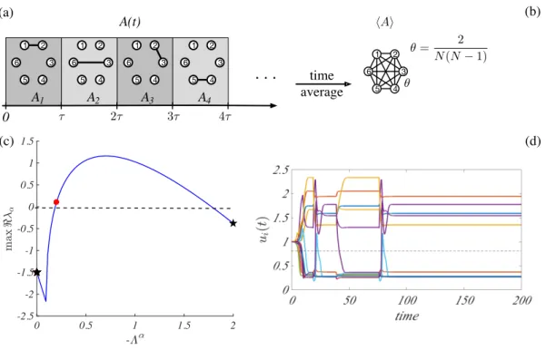
A(t) (a) 1 2 5 4 6 31 hAi (b) 0 0.5 1 1.5 2 -2.5 -2 -1.5 -1 -0.5 0 0.5 (c) (d) J = @F |hom eq+hLi J ~v = ~vFIG. 1: Twin network. Panel a): T -periodic network built from two static networks, of adjacency matrices A1and A2. Each
network in this illustrative example is made of N = 6 nodes. In the network stored in matrix A1, symmetric edges are drawn
between the pairs (1, 2), (3, 4) and (5, 6). The second network, embodied in matrix A2, links nodes (6, 1), (2, 3) and (4, 5). For
t2 [0, T ) the T -periodic network coincides with A1, A(t) = A1, while in [ T, T ) we set A(t) = A2. The time varying network
is then obtained by iterating the process in time. Panel b): the ensuing time average networkhAi = A1+ (1 )A2. Panel
c): dispersion relation (max< ↵vs. ⇤↵) or the average network (red circles), for each static twin network (black stars) and
for the continuous support case (blue curve). Here, the networks are generated as discussed above but now N = 50. Panel d): patterns in the average network. Nodes are blue if they present an excess of concentration with respect to the homogeneous equilibrium solution ((ui(1) u)¯ 0.1) and red otherwise ((ui(1) ¯u) 0.1). The outer drawing represents the entries of
~v, the eigenvector of the Jacobian matrixJ associated to the eigenvalues that yields the largest value of the dispersion relation. The black ring stands for the zeroth level; red-yellow colours are associated to positive entries of ~v, while blue-light blue refer to negative values. The reaction model is the Brusselator with b = 8, c = 10, Du= 3 and Dv= 10. The homogeneous equilibrium
is ¯u = 1 and ¯v = 0.8. The remaining parameters are set to = 0.3, T = 1, Du= 3 and Dv= 10.
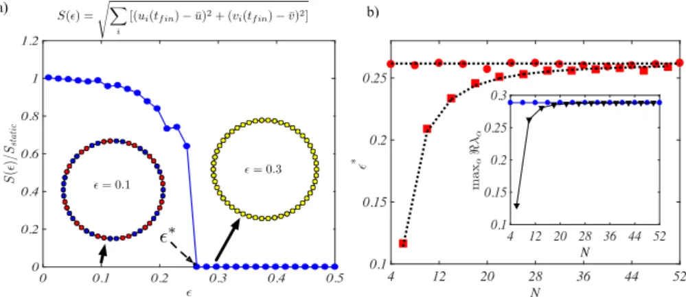
0 0.1 0.2 0.3 0.4 0.5 0 0.2 0.4 0.6 0.8 1 1.2 a) S(✏) = X b) i [(ui(tf in) ¯u)2+ (vi(tf in) ¯v)2] ✏ = 0.1 ✏ = 0.3 ✏⇤ 4 12 20 28 36 44 52 N 0.1 0.15 0.2 0.25 * 4 12 20 28 36 44 52 N 0.1 0.15 0.2 0.25 0.3
FIG. 2: The critical threshold ✏⇤. Panel a): pattern amplitude, S(✏), as a function of ✏ normalised to the amplitude of the
pattern for the averaged networkhAi = A1+ (1 )A2, for a T -periodic twin–network made of N = 50 nodes. Insets:
asymptotic patterns (u variable) for ✏ = 0.1 < ✏⇤; blue (resp. red) nodes represent an high (resp. low) concentration of u, with respect to the homogeneous equilibrium. For ✏ = 0.3 > ✏⇤, the system converges toward the homogeneous equilibrium; nodes are plotted in yellow when the concentration of species u is close to the homogeneous value. The employed reaction model is again the Brusselator and parameters are set as in Fig. 1. Panel b): ✏⇤ vs. N . The black dotted lines are drawn after equation (6), while the red symbols (circles for N/2 even and square for N/2 odd) are numerically computed. Inset: the maximum of the dispersion relation as a function of the network size (blue circles for N/2 even and black down-triangles for N/2 odd).
In the SI, we show that each term of the series can be readily computed based on the corresponding term of the Magnus series with ✏ = 1. By evaluating the solution over
one period ✏T we obtain
5 Moreover, it is known that ✏(✏T ) = 0. The stability
of the homogeneous solution is therefore determined by the eigenvalues of H✏, the so-called characteristic
expo-nents of the system. If the network varies smoothly, the threshold value (6) can thus be written as ✏⇤= min{✏ > 0 :8 > ✏ : max 2 < 0}, where is the spectrum
of H .
Note that for sufficiently small ✏, H✏ = H1,1 +O(✏)
where H1,1 = T1R T
0 M(t) dt = @XF (¯u, ¯v) +hLi is the
modified Jacobian matrix that applies to the averaged system. The eigenvalues of H✏ are hence close to those
of H1,1 and the periodic, continuously time varying
sys-tem behaves as the average one. We have hence recovered our main result. Finally, we emphasise that the analy-sis readily extends to the case of non-periodically time varying networks. The only requirement is the existence of the generalised average hLi = limT!1T1
RT 0 L(t)dt.
Relevant examples are addressed in the SI and include (i) quasi-periodic time dependent networks, (ii) networks constructed using aperiodic infinite words from a binary alphabet, and (iii) randomly switching networks. The latter example is directly inspired by epidemics systems evolving on social contact networks.
In conclusion, we have here shown that, by properly tuning the network topology over time, one can drive the emergence of self-organised patterns, following a Turing instability. The reaction-di↵usion system endowed with a time varying support behaves as its average analogue, provided the network dynamics is made sufficiently fast. Hence, patterns are obtained for a model attached to a network that changes over time, if they are predicted to occur on the associated average system. This is a novel route to pattern formation that we conjecture relevant for all those applications where di↵erent species interact via a network that can adjust in time, as follows either an endogenous or exogenous drive [42].
Acknowledgments The work of T.C. presents research results of the Belgian Network DYSCO (Dynamical Sys-tems, Control, and Optimization), funded by the In-teruniversity Attraction Poles Programme, initiated by the Belgian State, Science Policy Office. The scientific re-sponsibility rests with its author(s). D.F. acknowledges financial support from H2020-MSCA-ITN-2015 project COSMOS 642563.
[1] A. Pikovsky, M. Rosenblum, J. Kurths, Synchronization, Cambridge University Press, Cambridge, (2001). [2] J. D. Murray, Mathematical Biology II: Spatial
Mod-els and Biomedical Applications, 3rd Edition, Springer– Verlag, (2003).
[3] M. C. Cross, P. C. Hohenberg, Rev. Mod. Phys., 65, 851, (1993).
[4] A. M. Turing, Philos. Trans. R. Soc. London Ser. B, 237, 37, (1952)
[5] M. Mimura, J. D. Murray, J. Theor. Biol., 75, 249, (1978).
[6] M. Baurmann, T. Gross, U. Feudel, J. Theor. Biol.,245, 220, (2007).
[7] H.G. Othmer and L. E. Scriven, J. Theor. Biol. 32, 507-37 (1971)
[8] H.G. Othmer and L.E. Scriven, J. Theor. Biol. 43, 83-112 (1974)
[9] W. Horsthemke, K. Lam and P.K. Moore, Phys. Lett. A 328, 444–451 (2004)
[10] P.K. Moore and W. Horsthemke, Physica D 206, 121–144 (2005)
[11] H. Nakao and A. S. Mikhailov, Nature Physics 6, 544 (2010).
[12] M. Wolfrum, Physica D 241 (16), 1351-1357 (2012) [13] M. Asllani et al., Nat Comm, 5, 4517, (2014).
[14] S. Hata, H. Nakao and A. S. Mikhailov, Scientific Reports 4, 3585 (2014)
[15] S. Hata and H. Nakao, Scientific Reports 7, 1121 (2017) [16] M. Asllani et al., Physical Review E - Statistical, Non-linear, and Soft Matter Physics, 90 (4), 042814, (2014) [17] N.E. Kouvaris, S. Hata and A. Diaz-Guilera, Scientific
Reports 5, 10840 (2015)
[18] P. Holme, and J. Saram¨aki, Phys. Rep., 519, 97, (2012). [19] P. Holme, EPJB, 88, 234 (2015).
[20] J.-C. Delvenne, R. Lambiotte, and L. E. C. Rocha, Nat Comm, 6, 7366, (2015).
[21] N. Masuda and R. Lambiotte, A Guide to Temporal Net-works, Complexity Science ,World Scientific publishing, (2016).
[22] N. Perra et al, Phys. Rev. Lett., 109, 238701, (2012). [23] M. Starnini et al, Phys. Rev. E, 85, 056115, (2012). [24] N. Masuda, K. Klemm and V. Egu´ıluz, Phys. Rev. Lett.,
111, 188701 (2013)
[25] D. Stilwell, E. Bollt, and D. Roberson, SIAM J. Applied Dynamical Systems 5, 1 (2006)
[26] G. Vankeerberghen, J. Hendrickx and R. Jungers, http://dx.doi.org/10.1145/2562059.2562124
[27] D. Liberzon and A.S.Morse, IEEE Control Systems, 19, 59, (1999).
[28] A. Barrat et al, The European Physical Journal Special Topics, 222, (6), 1295, (2013)
[29] A. Barrat et al, Clinical Microbiology and Infection, 20, (1), 10, (2014)
[30] P. So, B.C. Cotton and E. Barreto, CHAOS, 18, 037114, (2008).
[31] S. Boccaletti, D.-U. Hwang, M. Chavez, A. Amann, J. Kurths, and L. M. Pecora, Phys. Rev. E, 016102 (2006) [32] V. Kohar et al., Phys. Rev. E, 90, 022812, (2014). [33] W. Magnus, Comm. Pure and Appl. Math. VII (4), 649,
(1954).
[34] S. Blanes, F. Casas, J. A. Oteo and J. Ros, Physics Re-ports 470, 151, (2009).
[35] F. Casas, J. A. Oteo and J. Ros, J. Phys A: Mathematical and General 43, 3379, (2001)
[36] F. Verhulst, Nonlinear Di↵erential Equations and Dy-namical Systems, Springer (1996).
[37] A. S. Morse, Supervisory control of families of linear set-point controllers—part 1: exact matching, IEEE Trans. Automat. Contr., vol. 41 (1996), pp. 1413–1431
[38] P. C. Moan and J. Niesen, Convergence of the Magnus series, Found Comput. Math 8 (2008), pp. 291–301 [39] S. Klarsfeld, J. A. Oteo, Recursive generation of
(1989), pp. 3270–3273.
[40] S. Blanes, F. Casas and J. Ros, Improved high order inte-grators based on the Magnus expansion, J. BIT Numerical Mathematics 40, 3 (2000), pp. 434-450
[41] A closed approximate formula for ✏⇤can be also derived relying on the mechanism used in the proof of the
aver-aging theorem, as discussed in the SI.
[42] See Supplemental Material [url] for a detailed proof of the main result, the computation of the critical threshold and an extension of our result to non-periodic and random temporal networks. The SI includes Refs. [36-40].
Supplementary Information - The theory of Turing patterns on time varying networks
Julien Petit1,2, Ben Lauwens2, Duccio Fanelli3,4, Timoteo Carletti1
1naXys, Namur Institute for Complex Systems,
University of Namur, Belgium
2Department of Mathematics,
Royal Military Academy, Belgium
3Dipartimento di Fisica e Astronomia and CSDC,
Universit`a degli Studi di Firenze, Italy
4INFN Sezione di Firenze, Italy
I. PROOF OF THE MAIN RESULT
The aim of this section is to provide a formal statement and a detailed derivation of our main result that we will cast in the form of a theorem. Let us first recall the definition of the model and then proceed to prove the theorem.
We assume, for the sake of simplicity, two di↵erent species that live and interact on a periodically time varying network. The number of nodes N is kept fixed, while pairwise weighted links adjust in time. The network structure is embedded in a periodic time varying weighted adjacency matrix Aij(t), that results in time varying link strength,
si(t) =PjAij(t). Further, we introduce the time varying Laplacian matrix defined Lij(t) = Aij(t) si(t) ij. Observe
that for all t one hasPjLij(t) = 0, namely L(t) is a row stochastic matrix.
Species di↵use across the network and interact on the same node as dictated by specific nonlinear reaction terms. The model (equations (1) in the main body of the paper) reads:
˙ui= f (ui, vi) + Du N X j=1 Lij(t/✏)uj ˙vi= g(ui, vi) + Dv N X j=1 Lij(t/✏)vj (1)
where f and g are nonlinear functions and Du and Dv denote the di↵usion coefficients associated, respectively, to
species u and v. The parameter ✏ sets the rate of the network evolution. For a subsequent use let us rewrite the above system in a more compact form by defining the 2N –dimensional vector ~x = (u1, . . . , uN, v1, . . . , vN):
˙~x(t) = F (~x) + L(t/✏)~x , (2)
where F (~x) = (f (u1, v1), . . . , f (uN, vN), g(u1, v1), . . . , g(uN, vN))T and
L(t)~x :=⇣DuL(t) 0
0 DvL(t) ⌘
~x . (3)
To study the emergence of patterns for model (1), as follows a symmetry breaking instability of the Turing type, one cannot invoke the standard machineries, as eigenvectors and eigenvalues depend on time. To compute the dispersion relation following the canonical approach additional assumptions are to be enforced, as e.g. discussed in [31]. To avoid this, we proceed with an alternative route which involves dealing with the so called theorem of averaging hereafter recalled for consistency (the interested reader can consult e.g. [36] for further details on this topic):
Theorem 1 (Averaging in the periodic case) Let us consider the system
˙x = ✏f (t, x) , x(0) = x02 D ⇢ Rn, (4)
where f and @xf are defined, continuous and bounded in [0,1) ⇥ Rn and assume f (t,·) to be T -periodic.
Let hfi(y) be the time average of f(t, y), that is hfi(y) =T1
Z T 0
f (t, y) dt , (5)
and let y(t) be the solution of
˙y = ✏hfi(y) , y(0) = x02 D ⇢ Rn.
Based on the above theorem, and as discussed in the main body of the paper, we can relate the behaviour of system (1) to the behaviour of its averaged homologue, defined by replacing L(t) with the time averaged operatorhLi defined as:
hLi = T1 Z T
0
L(t) dt , (6)
where T > 0 is the period. As a side remark, we anticipate that our result holds true also if the time evolution of the network is not periodic, provided a generalised average exists, namely:
hLi = limT !1 1 T Z T 0 L(t) dt . More precisely we can state and proof the following theorem
Theorem 2 (Main result) Let us define the averaged system [1]:
˙~x(t) = F (~x) + hLi~x , ~x(0) = ~x02 R2N, (7) where ~x = (u1, . . . , uN, v1, . . . , vN),hLi = ⇣D uhLi 0 0 DvhLi ⌘
andhLi is defined using Eq. (6). Assume moreover that the above system exhibits Turing patterns, namely that a stable homogeneous equilibrium ¯x = (¯u, . . . , ¯u, ¯v, . . . , ¯v) of system (7) can turn unstable, for an appropriate choice of the parameters involved, upon application of a non homogeneous perturbation.
Then there exists ✏⇤> 0 such that the fast varying version (see Eq. (2)) displays Turing patterns for all 0 < ✏ < ✏⇤.
Proof Let us first introduce the rescaled time ⌧ = t/✏ and the adapted variables ~w(⌧ ) = ~x(t)|t=✏⌧, to rewrite
Eq. (2) as (with the notation0= d/d⌧ ):
~
w0(⌧ ) = ✏ [F ( ~w) +L(⌧) ~w] . (8) We can then apply Theorem 1 and obtain
~
w(⌧ ) ~y(⌧ ) =O(✏) , for all 0 < ✏ < ✏⇤, where ~y(⌧ ) is the solution of the averaged system
~y0(⌧ ) = ✏ [F (~y) +hLi~y] , ~y(0) = ~w(0)2 R2N. (9)
Back to the original variables, ~x and time t, the last statement can be rephrased as follows. Let ~x be the solution of Eq. (2) and ~z(t) = ~y(t/✏) the solution of Eq. (7) with the same initial conditions, then
~x(t) ~z(t) =O(✏) for all 0 < ✏ < ✏⇤ and t =O(1).
Namely the two above orbits stay close over a macroscopic time window. Hence, if a symmetry breaking instability occurs for system (7), paving the way to the subsequent pattern derive, the same holds for the original system (2).
II. ON THE CRITICAL THRESHOLD ✏⇤.
The aim of this section is to provide a detailed derivation of the formulae employed in the main text to estimate ✏⇤. To this end we consider again the reference system written in a compact vector form (see Eq. (2))
Assume there exists ¯u, ¯v such that ¯x = (¯u, . . . , ¯u, ¯v, . . . , ¯v)T is an homogeneous equilibrium of (2), and write
~x = ~x x to denote a tiny perturbation. Linearising system (2) close to the homogeneous solution yields:¯
˙~x = M✏(t) ~x with M✏(t) = @xF (¯x) +L(t/✏) , (10)
where @xF (¯x) is the Jacobian matrix of F evaluated at ¯x.
In the rest of the section we assume that no Turing instability is allowed for ✏ = 1. In other words, the imposed perturbation fades away when ✏ is set equal to 1, and system (2) converges to its homogeneous equilibrium. At variance, the time averaged system, which corresponds to the limiting case ✏⇡ 0, can exhibit patterns of the Turing class. In the following, we write for short M✏=1= M. Our goal is to compute, in this setting, the critical threshold for
3
A. Temporal network of contact sequences
Let us consider a finite collection of networks indexed by k2 K and label L[k] : k2 K their associated Laplacian
matrices. For fixed reaction terms, we then define, for every k 2 K, the matrix M[k] = @
xF (¯x) +L[k], where
L[k] = ⇣DuL[k] 0
0 DvL[k] ⌘
. We further assume that for every linearised system involving a given M[k], i.e. when the
index k is kept fixed, the zero solution is stable with respect to a small non homogeneous perturbation ~x.
Let us now introduce a switching signal, (t), that is, a piecewise constant function : [0,1) ! K. This provides a direct map between time and indexes, thus enabling us to associate to each time its corresponding network
L(t) = L[ (t)]. (11)
Working along these lines, we generalise the construction of twin network as discussed in the main body of the paper. For the twin network, in fact, K = {1, 2} and (t) = 1 if mod(t, T )/T 2 [0, ) and (t) = 2 otherwise. We are thus interested in the stability of the 1-parameter family of linearised systems
˙~x = M[ (t)]
✏ ~x with M[ (t)]✏ = @xF (¯x) +L[ (t/✏)]. (12)
If the interval between any two consecutive discontinuities of (t) is (on average) above a given threshold ⌧D, called
the dwell time of the system, then the zero solution of Eq. (12) is stable (see for instance [37]).
Let 0 = t0< t1< t2< . . . be the times of discontinuities of (t), and define ⌧k by tk+ ⌧k+1= tk+1for k2 N. The
switching signal (t) is constant over every interval [tk, tk+1) and therefore the solution of Eq. (12) can be explicitly
computed as
~x(✏tk+1) = exp(✏⌧k+1M[ (✏t✏ k)]) ~x(✏tk), k2 N . (13)
We then get a discrete time system that is stable under injection of a small non homogeneous perturbation, if the joint spectral radius satisfies:
⇢nexp(✏⌧kM[ (✏t✏ k)]), k2 N)
o
< 1 . (14)
Observe that even for a set composed by only two matrices, the joint spectral radius is cumbersome to compute [26]. To allow a more straightforward computation of the critical threshold ✏⇤, we proceed by making the simplifying
assumption that the switching signal (t) has a finite number of discontinuities (n) and it is T periodic, with T =Pni=1⌧i.
As a result, we have that the solution of (13) at every integer multiple of periods ✏mT is given by
~x(m✏T ) = (Q✏(✏T ))m ~x(0) . (15)
The time-evolution operator over one period, Q✏(✏T ) = n Y k=1 exp(✏⌧kM[ (✏t✏ k 1)]) = n Y k=1 exp(✏⌧kM[ (tk 1)]) ,
where we have used that M[ (t)]✏ = M[ (t/✏)] and thus M[ (✏t)]✏ = M[ (t)] (see Eq. (12)).
The critical value of the acceleration parameter ✏ is thus given by
✏⇤= min{✏ > 0 : 8s ✏, ⇢(Qs(sT )) 1} , (16)
where ⇢ denotes the spectral radius.
B. Continuously varying networks
We now consider the more general case of a continuously time varying network, with Laplacian matrix L(t) whose entries are integrable functions of time. The solution of the linearised system with ✏ = 1,
can be written as ~x(t) = exp ✓Z t 0 M(t) dt ◆ ~x(0) , (18)
if and only if the matrices M(t1) and M(t2) commute for any pair t1, t2. Let us observe that, as M contains both a
term related to the reactions and another related to the di↵usion, the above assumption may not be satisfied, even if the Laplacian matrices associated to the networks do commute: the commutation between the Laplacian matrix and the reaction part is also needed. However one can write:
~x(t) = exp (⌦(t)) ~x(0) , (19)
where ⌦(t) =P1n=1⌦n(t), is known as the Magnus expansion [33,34]. From
d⌦(t) dt = 1 X n=0 Bn n!ad n ⌦A , (20)
where the Bn’s are the first Bernoulli numbers (B1 = 1/2), adXA = [X, A] = XA AX denote the matrix
commutator and ad0XA = A, adkXA = [X, adk 1X A], one can iteratively compute all the terms of the series. For
example, ⌦1(t) = Z t 0 M(t1)dt1 (21) ⌦2(t) = 1 2 Z t 0 Z t1 0 [M(t1), M(t2)] dt2dt1 (22) ⌦3(t) = 1 6 Z t 0 Z t1 0 Z t2 0 ([M(t1), [M(t2), M(t3)]] + [M(t3), [M(t2), M(t1)]]) dt3dt2dt1. (23)
One can also prove [38] the convergence of the above series providedR0tkM(⌧)k2d⌧ < ⇡.
As previously done when dealing with the switching network case, we assume for simplicity that the network evolution is periodic. Hence, the entries of L(t) are T periodic continuous functions. The Floquet theorem ensures thus that the solution of (17) can be written as
~x(t) = P(t) exp (tF) ~x(0) , (24)
where P is T -periodic and bounded, and F does not depend on time. The asymptotic stability of the null solution is determined by the eigenvalues of F, known as the characteristic exponents of the system. The Floquet-Magnus expansion [35] allows one to write
~x(t) = exp (⇤(t)) exp (tF) ~x(0) , (25)
where the involved matrices are obtained as the sums of series [2] ⇤(t) = 1 X n=1 ⇤n(t), F = 1 X n=1 Fn. (26)
The matrix ⇤(t) is T -periodic, with ⇤(0) = 0. Since ~x(T ) = exp[⌦(T )] ~x(0), we have the identity:
Fn= ⌦n(T )/T, n 1 . (27)
Let us now consider system (10) in the case ✏ < 1. We write ⌦✏(t) for the Magnus expansion corresponding to
M✏(t) = M(t/✏), and apply the same notation to ⇤(t) and F. This leads to
~x(t) = exp 1 X n=1 ⇤✏,n(t) ! exp t 1 X n=1 F✏,n ! ~x(0) , (28)
where ⇤✏(t) is ✏T -periodic, and
5 The stability is determined by the eigenvalues of the characteristic exponent ✏T F✏, or equivalently, by looking at the
sign of the real part of the eigenvalues of ⌦✏(✏T )/(✏T ).
Let us observe that for every n 1, we have ⌦✏,n(✏t) = ✏n⌦n(t). In conclusion we obtain
⌦✏(✏T ) = 1
X
n=1
✏n⌦n(T ) , (30)
and, as a consequence, the stability of the zero solution of the fast-varying system (✏ < 1) is determined by the sign of the real part of the eigenvalues ofP1n=1✏n 1⌦(T )/T .
As remarked when discussing the implication of the averaging theorem, in the limiting case ✏! 0, the averaged network can be used to determine the stability of the system. Indeed, if ✏ > 0 is small enough, the eigenvalues of P1
n=1✏n 1⌦n(T )/T = ⌦1/T + o(✏) lie on the same portion of the imaginary axis as the eigenvalues of
⌦1 T = 1 T Z T 0 M(t) dt = @xF (¯x) +hL(t)i. (31)
The critical value of ✏ can be computed by imposing ✏⇤= min
⇢
✏ > 0 : > ✏ =) max
2 < 0 (32)
where is the spectrum of (30) for ✏ = .
The computation of the first terms of the Magnus expansion, truncated as desired so as to reach the necessary precision on ✏⇤, can be carried out by using the recursive formulas first obtained in [39]
⌦n= n 1 X j=0 Bj j! Z t 0 S(j)n (t1)dt1, n 1 (33)
where the S(j)n follow from the recursion
S(j)n = n j X m=1 h ⌦m, S(j 1)n m i , 1 j n 1 (34) S(0)1 = M(t) (35) S(0)n = 0, n > 1. (36)
Working out these formulas explicitly, ⌦n(t) = n 1 X j=1 Bj j! X k1+...+kj =n 1 k1 0,...,kj 0 Z t 0 ad⌦k1(⌧ )ad⌦k2(⌧ ). . . ad⌦kj(⌧ )M(⌧ )d⌧, n 2. (37)
The above formulas are straightforward to implement, but prove numerically heavy to calculate since they involve multiple integrals of nested commutators. To overcome this limitation one can use the Time-stepping method which consists in performing a partition of the interval [0, T ] in m subintervals of length h and then compute the Taylor series for M(t) using the midpoint t[k] = (k 1)h +h
2 = (k 1 2)h: M(t) = 1 X j=0 m[k]j (t t[k])j, tk 1 t < tk, with m[k]j = 1 j! djM(t) dtj t=t[k] . (38)
Inserting this relation into the recursive formulas given above yields [40], up to order 5: ⌦[k]1 = hm[k]0 + h3 1 12m [k] 2 + h 5 1 80m [k] 4 + o(h 7) (39) ⌦[k]2 = h3 1 12 h m[k]0 , m [k] 1 i + h5 ✓ 1 80 h m[k]0 , m [k] 3 i + 1 240 h m[k]1 , m [k] 2 i◆ + o(h7) (40) ⌦[k]3 = h5 ✓ 1 360 h m[k]0 , m [k] 0 , m [k] 2 i 1 240 h m[k]1 , m [k] 0 , m [k] 1 i◆ + o(h7) (41) ⌦[k]4 = h5 1 720 h m[k]0 , m [k] 0 , m [k] 0 , m [k] 1 i + o(h7). (42)
Here, we have used the simplified notation [x1, x2, . . . , xj] = [x1, [x2, [. . . , [xj 1, xj] . . .]]]. Over each time interval
[tk 1, tk), we get as a viable approximation to the time evolution operator from ~x(tk 1) to ~x(tk), relative to the
reference case ✏ = 1 : exp (⌦(tk, tk 1)) = exp 4 X n=1 ⌦[k]n + o(h7) ! (43) After appropriate truncation of the series, we have
~x(T ) = m Y k=1 exp 0 @X n 1 ⌦[k] n 1 A ~x(0) . (44)
Note that here no integration of M(t) is required, so the computation is much faster to handle numerically. The analysis can be readily extended to the setting ✏ < 1. If one considers again m subintervals [3] in [0, ✏T ], we then have
~x(✏T ) = m Y k=1 exp 0 @X n 1 ⌦[k]✏,n(✏tk, ✏tk 1) 1 A ~x(0) = m Y k=1 exp 0 @X n 1 ✏n⌦[k]n (tk, tk 1) 1 A ~x(0) . (45) As before, we only need to compute the terms of the Magnus series for the original system, that we then multiply by the appropriate integer power of ✏. In doing so, we can obtain an estimate for the critical value ✏⇤ by evaluating the
spectral radius of the matrix that appears in the right hand side of the latter equation.
C. A closed-form approximate expression for ✏⇤
The aim of this section is to present an alternative method, directly inspired by the proof of the averaging theorem, to compute the critical threshold ✏⇤. This procedure avoids dealing with the computation of the monodromy matrix and returns a closed formula for ✏⇤, which proves adequate versus numerical simulations.
Digging into the proof of the averaging theorem reveals that it relies on an invertible change of coordinates matching the two systems (Eq. (8) and Eq. (9)). Our idea is hence to quantify ✏⇤ by determining the range of ✏ for which the
sought invertibility can be achieved. The required change of variables is given by ~
w = ~y + ✏~u(⌧, ~y) , (46)
where ~u is explicitly given by
~u(s, ~y) = Z ⌧
0
[L(r)~y hLi~y] dr , (47)
where the terms involving the reaction part, F in Eq. (2), cancel out because they do not explicitly depend on time. To be able to invert relation (46) one has to require that its Jacobian
J(✏) = @ ~w
@~y =I + ✏@y~u ,
is non singular, namely that det J6= 0. This is certainly true if ✏ = 0. We could hence determine an upper bound for ✏ as:
✏⇤= min{✏ > 0 : 8q 2 [0, ✏) , det J(q) 6= 0} . (48) By using the form for ~u given by Eq. (47) one can obtain
J(✏) =I2N + ✏@y~u =I2N + ✏
Z ⌧ 0
[L(r) hLi] dr , and recalling the explicit form ofL we get:
det(I2N+ ✏@y~u) = 0, det
✓ IN + ✏Du Z ⌧ 0 [L(r) hLi] dr ◆ det ✓ IN+ ✏Dv Z ⌧ 0 [L(r) hLi] dr ◆ = 0 . (49) In the following we apply this strategy to compute ✏⇤ for the twin network setting introduced in the main body of the paper.
7
D. The critical threshold for the twin network
The analysis presented in the previous section II C can be pushed further in the case of switching twin–network (see main body of the paper for technical details on the model formulation). In this case we can exactly compute hLi = L1+ (1 )L2 and thus the right hand side of Eq. (49). In fact let
(s) = Z s 0 [L(r) hLi] dr , then we have (s) = ( (1 )(L1 L2)t if{t/T } 2 [0, ) (T t)(L1 L2) if{t/T } 2 [ , 1) , where{r} denotes the fractional part of the real number r.
Let ⇤↵
12, ↵ = 1, . . . , N , be the eigenvalues of L1 L2, then the roots of Eq. (49) depend on t and are of the form
(we assume to order the eigenvalues such that ⇤1 12= 0) ✏↵= 1 ⇤↵ 12 1 Du (t) or ✏↵= 1 ⇤↵ 12 1 Dv (t) , 8↵ = 2, . . . , N and t > 0 , where (t) = ( (1 )t if{t/T } 2 [0, ) (T t) if{t/T } 2 [ , 1) , which has a minimum at t = T . Hence Eq. (48) returns:
✏⇤⇡ ⇤N 1 12 (1 )T min 1 Du, 1 Dv , (50) where we set ⇤N
12 = max↵|⇤↵12|, keeping in mind that the spectrum of L1 L2 contains both positive and negative
eigenvalues.
III. ANOTHER APPLICATION: THE BLINKING NETWORK
Many interactions involving humans can be described by a binary contact lasting for a finite amount of time after which the two individuals get apart (contact networks) [28,29]. During these events information can be mutually shared. If contacts are not mediated by electronic devices, viruses can pass from an individual to the other, hence triggering the epidemic spreading. As a first approximation, the dynamics of interaction within an large community can be broken down into a collection of successive pairwise exchanges, that extend over a finite window of time. Working in this setting, it is interesting to elaborate on the conditions (e.g. characteristic time of interactions) that discriminate between an homogenous or pattern like (in terms of virus load or information content) asymptotic equilibrium. Let us observe that typical time scales of social contacts are of the order of minutes or hours, hence faster than the typical time of virus incubation.
To this end we here consider a collection of networks, each made of N isolated nodes with the exception of two nodes that are connected via an undirected link. Any two networks in this collection di↵er because a di↵erent link is activated. There are hence N (N 1)/2 di↵erent networks in total. All networks have the same Laplacian spectrum given by ⇤1 = 0 with multiplicity N 1 (i.e. the number of connected components the network is made of) and
⇤N = 2 with multiplicity 1 (i.e. the minimal value the eigenvalues can assume in the case of complete bipartite
network).
Let us now define a periodically time varying network A(t) as follows. Fix a period T > 0 and divide the interval [0, T ] into m = N (N 1)/2 equal disjoint subintervals ⌧i,[i⌧i= [0, T ] and ⌧i\ ⌧j=; if i 6= j. Hence, |⌧i| = ⌧ = T/m
(of course this assumption can be relaxed and subintervals with di↵erent length allowed for). Assume to order the networks in the collection from 1 to N (N 1)/2, then define A(t) by
where Aiis the adjacency matrix associated to one of the networks of the collection. Then we periodically repeat the
procedure, i.e. if t > T then consider (t mod T ) instead of t. Di↵erently stated, during each time interval, a novel link is created between a newly selected pair of nodes and the connection active during the preceding time window deleted. Hence, at each time there is one and only one active link (see top left panel of Fig. 1 for an illustrative explanation). By making use of the aforementioned notation, we could also say A(t) = A[ (t)], where (t) = i if
t2 ⌧i. Because of the assumption of equal length intervals ⌧i, the adjacency matrix of the averaged network is given
by
hAiij =
( 2
N (N 1) if i6= j
0 if i = j , (52)
while the Laplacian matrix reads
hLiij = ( 2 N (N 1) if i6= j 2 N if i = j , (53)
whose spectrum is ⇤1= 0 with multiplicity 1 and ⇤N = 2/(N 1) with multiplicity N 1. One can thus choose the
network size N to ensure that the relation dispersion admits a positive real part, once evaluated in ⇤N = 2/(N 1)
(see bottom left panel of Fig. 1).
To carry out one test we consider again the Brusselator model running on top of a such time varying network. The reaction terms read therefore f (u, v) = 1 (b + 1)u + cu2v and g(u, v) = bu cu2v, where b, c are parameters of the
model fixed that we assign to be b = 8 and c = 10. The homogeneous equilibrium is thus ¯u = 1 and ¯v = 0.8. The di↵usion coefficients are set to Du= 3 and Dv = 10.
We also assign the remaining model parameters in such a way that each network of the collection (Ai) cannot
yield Turing patterns. This amounts to requiring 1 = < (⇤1) < 0 (the homogeneous equilibrium is stable) and N =< (⇤N) < 0 (see bottom left panel of Fig. 1).
Applying Theorem 2 one can find a positive ✏⇤ such that for all 0 < ✏ < ✏⇤, the fast varying time dependent
system (2) exhibits Turing patterns. This is due to the fact that, under this operating condition, system (2) is close enough to its averaged analogue to be able to follow its orbits. Conversely, system (2) does not exhibit Turing patterns if ✏ is too large (see bottom right panel of Fig. 1).
IV. NON-PERIODIC NETWORKS
Our main result, Theorem 2, holds true also if the time varying network is not periodic: as mentioned earlier, we solely require the existence of the generalised average
hLi = limT !1 1 T Z T 0 L(t) dt . (54)
The aim of this section is thus to shortly discuss some examples of a non-periodic time-varying networks for which Eq. (54) is well defined.
The first example exploits the non commensurability of the periods of two periodic networks. More precisely, let G1(t), respectively G2(t), be a T1, respectively T2, periodic network. Then, assuming T1/T2 62 Q, the network
G(t) = G1(t) + G2(t) is quasi-periodic and one easily obtains that
hLi = hL1i + hL2i ,
wherehLii is the average Laplacian matrix of the i–th network, computed over the period Ti.
Building on this setting one could generate interesting applications. Imagine that for all finite t, the network associated to G(t) cannot develop patterns. Then we could speculate on the possibility that patterns arise in the averaged network in the limit t! 1. For instance, given two adjacency matrices A1 and A2 and two parameters
j2 (0, 1), j = 1, 2, we define
Gj(t) =
(
A1 if{t/Tj} 2 [0, j)
A2 if{t/Tj} 2 [ j, 1) ,
then G(t) = G1(t) + G2(t) is quasi-periodic. For all finite t no patterns are allowed on G(t) if they are not observed
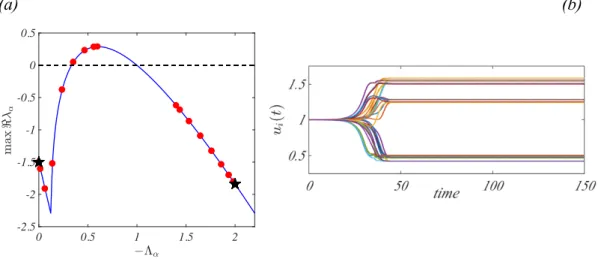
9 0 0.5 1 1.5 2 --2.5 -2 -1.5 -1 -0.5 0 0.5 1 1.5 time average 1 2 5 4 6 3 = 2 N (N 1) hAi (b) (c) (d) 2⌧ 3⌧ 0 ⌧ 1 2 5 4 6 3 1 2 5 4 6 3 A1 A2 A3 A4 1 2 5 4 6 3 1 2 5 4 6 3
. . .
A(t) (a) 4⌧ (c)FIG. 1: Blinking network. Panel a): T -periodic network built by using m networks, Ai i = 1, . . . , m (m = N (N 1)/2). In
this example, each network is made by N = 6 nodes among which only two are connected. Let ⌧ = T /M , then for t2 [0, ⌧) the T -periodic network coincides with A1, in the successive interval t2 [⌧, 2⌧), A(t) = A2, and so on. The time varying network
is then obtained by periodically repeating this construction. Panel b): the time average networkhAi = KN/M , where KN
denotes the complete network made by N = 6 nodes in this example. Panel c): dispersion relation for the average network (red circles), for each static network Ai (black stars) (N = 11 nodes) and for the continuous support case (blue curve). Panel d):
the time evolution of the concentrations ui(t) for the blinking network composed by N = 11 nodes. The reaction dynamics is
given by the Brusselator model (f (u, v) = 1 (b + 1)u + cu2v and g(u, v) = bu cu2v where b, c are parameters of the model
hereby fixed to b = 8 and c = 10); the homogeneous equilibrium is ¯u = 1 and ¯v = 0.8. The remaining parameters are T = 1, Du= 3 and Dv= 10.
still yield patterns for a suitable choice of j. We do not provide an explicit numerical evidence of this mechanism
here, but instead turn to consider a di↵erent model of non periodic networks. For this further example, a numerical realization will be also given to support the conclusion of the analysis.
The final example that we are going to illustrate is based on aperiodic words (or binary strings) and follows the construction of a map associating to the letters (or entries) of the word a network. Let us consider for the sake of simplicity, two time periodic networks built on two di↵erent time windows of identical total duration:
P0(t) = ( A1 if{t/T } 2 [0, ) A2 if{t/T } 2 [ , 1) and P1(t) = ( A2 if{t/T } 2 [0, 1 ) A1 if{t/T } 2 [1 , 1) (55) where T > 0 is the period and 2 (0, 1) a fixed parameter.
Given a string made of w = (in)n2N, in2 {0, 1}, we can finally obtain a time varying network by selecting P0 or P1
according to the entries appearing in w. The Laplacian matrix L(t) associated to this latter network will be aperiodic if the word w also is. On the other hand, because of the definition of P0 and P1 (they are based on windows of the
same length) one straightforwardly obtains: hLi = L1+ (1 )L2.
Let us conclude by providing an explicit example (see also Fig. 3). Let us call the complexity of w the application pw :N ! N which gives for every n the number of subwords of length n in w. Using the Morse-Hedlund theorem[4],
an aperiodic word w of minimal complexity is such that
8n 2 N, pw(n) = n + 1. (56)
w = 00101 . . .
0
T
2T
3T
4T
P
0
P
0
P
1
P
0
P
1
5T
A
0A
1A
0A
1A
1A
0A
0A
1A
1A
0{ { { { {
. . .
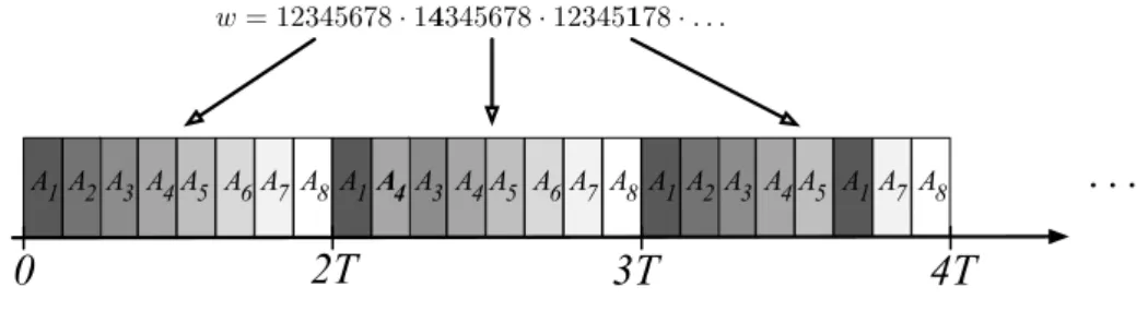
FIG. 2: Aperiodic time varying network build using a Sturmian words. From the top, the word w = 00101 . . . , the map that associates to each letter (entry) of the word (binary string) the network P0(t) or P1(t), the resulting aperiodic time varying
network.
wFibonacci= w
0w1w2. . . where the n–th letter, wn, is given by
wF ibonacci(n) = 2 +bn'c b(n + 1)'c where ' = 1 + p
5
2 . (57)
Observe that such word can be obtained using the following recursion
s0= 0, (58)
s1= 01, (59)
sn = sn 1· sn 2, 8n 2, (60)
where s1· s2 is the concatenation of s1 and s2, from which the name Fibonacci follows. A numerical realization of
the proposed scheme is reported in Figure 3: patterns appear in the time varying network also if they are formally impeded on each subnetworks components. Note that by considering low complexity words, when defining the network dynamics, the corresponding threshold value of ✏ is expected to be larger than with words with a higher complexity. We thus have a less demanding condition on the ratio between the time scales of the network and of the reactions, in order to generate patterns due to varying topology.
V. RANDOM TEMPORAL NETWORKS
The example based on the blinking network, as previously discussed, deals with the simplifying assumption that each contact lasts the same amount of time. Moreover, encounters are assumed to repeat periodically in time. This somehow unnatural hypothesis can be relaxed without a↵ecting our conclusion, as we will demonstrate in the following. More specifically, we will hereby revisit the blinking network example, assuming now random temporal switches.
For the sake of clarity let us consider the blinking network with five nodes. We select 8 among the 10 possible networks containing a single link, to represent the static configurations (see Fig. 4). The only requirement is that each node should participate at least once to the formation of a link to ensure the connectivity of the average network. We then construct a reference framework by implementing a deterministic evolution based on a fixed sequence of discrete switches, from 1 up to 8 using the natural ordering, that covers a finite interval of time T , called the period. Then, the dynamics is periodically repeated in time. Let us define a uniform partition of this period, ⌧i = T /8 for
all i, and use the Brusselator for the reaction kinetics. The chosen value of T is not relevant and it has been here set to 1. The system evolving on the average network,hAi =P8i=1Ai/8, fulfils the conditions for Turing instability.
Then, according to Theorem 2, Turing patterns also emerge over the temporal network if the switching is fast enough, ✏ < ✏⇤
det⇡ 0.37 (see Fig. 6, solid black line).
Let us now construct a randomly time varying blinking network, based on the 8 independent configurations as introduced above. More precisely, with a small abuse of language, we define a period T as a sequence of length 8 made by a random permutation of the integers{1, . . . , 8}. To each sequence we associate the corresponding ordered set of adjacency matrices. Then a new sequence, still of length 8, is drawn which applies to the next iteration and the whole procedure is eventually iterated. Given a sequence w(0) = i
11 0 0.5 1 1.5 2 -2.5 -2 -1.5 -1 -0.5 0 0.5
(a)
(b)
FIG. 3: Twin network and Fibonacci word. Using the twin network A1 and A2 (made by N = 32 nodes) and the Fibonacci
word wFibonacci = 00101001001 . . . , we apply the scheme presented in Fig. 2 to build a time varying aperiodic network A(t). Panel a): the dispersion relation (max< ↵ vs. ⇤↵) for the average network (red circles), for each static twin network (black
stars) and for the continuous support case (blue curve). Panel b): the time evolution of the concentrations ui(t) for the aperiodic
network composed by N = 32 nodes. The reaction dynamics is given by the Brusselator model (f (u, v) = 1 (b + 1)u + cu2v and g(u, v) = bu cu2v where b, c are parameters of the model fixed to b = 8 and c = 10); the homogeneous equilibrium is ¯
u = 1 and ¯v = 0.8. The remaining parameters are T = 1, Du= 3, Dv= 10 and ✏ = 0.01.
after
after
after
after
after
after
after
after
A
2
A
1
A
3
A
4
A
5
A
6
A
7
A
8
⌧
1
⌧
2
⌧
3
⌧
4
⌧
5
⌧
6
⌧
7
⌧
8
FIG. 4: Blinking network with N = 5 nodes and M = 8 configurations. The temporal ordering corresponds to a reference deterministic evolution; during one period T = ⌧1+ . . . + ⌧8, the adjacency matrix A(t) remains constant and equal to Ai(t)
for a duration ⌧i, i = 1, . . . , M .
k2 {0, . . . , 8} we define a new sequence w(1)= R
k(w(0)) obtained from w by replacing k of its entries with numbers
drawn with uniform probability from {1, . . . , 8} (repetitions are allowed). For instance if k = 1, then w(1) and w(0)
can di↵er at most by one symbol. We then repeat the process n times, starting always from the same initial sequence to obtain the sequences, w(j)= R
k(w(0)), j = 1, . . . , n, that are eventually concatenated to build a long enough one,
w = w(0)
· w(1)
· . . . · w(n). In this way we can ”continuously” pass from a deterministic, regular periodic setting (the
same sequence, initially drawn, of 8 integers is repeated over all time windows, hence k = 0) to a random one (each period a new sequence of 8 integers is randomly drawn, k = 8).
Given a sequence built using the latter recipe, we can define a randomly time varying blinking network by gen-eralising the construction done in the deterministic case, where now the sequence of adjacency matrices follows the entries of the random sequence (see Fig. 5). The same construction applies to the Laplacian matrix L(t).
. . .
w(1)= R 1(w(0)) = 14345678 w(0)= 12345678 w(2)= R 1(w(0)) = 12345178 w = 12345678· 14345678 · 12345178 · . . . A1A2A3A4A5 A6A7 A8A1A4A3A4A5 A6A7A8A1A2A3 A4A5 A1A7A84T
0
2T
3T
FIG. 5: Randomly time varying blinking network. From the top, the initial sequence w(0) = 12345678 and two possible new
sequences obtained from the initial one with k = 1, w(1)= 14345678 and w(2)= 12345178 (we denoted in bold the changed entries), the concatenated sequence w = w(0)
· w(1)
· w(2)
· . . . and the resulting sequence of adjacency matrices.
As already observed, if k = 1 two consecutive periods, i.e. two adjacent sequences of 8 integers, di↵er at most for two symbols. Then the deviation from periodicity (k = 0) can be considered small. Hence, the value of ✏⇤
rnd allowing
for Turing patterns on a randomly time varying network will be similar to the one obtained for the deterministic reference case ✏⇤det (compare the red squares and the black circles lines in Fig. 6). On the other hand, when the
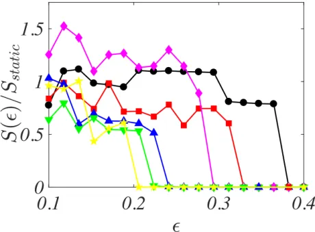
ordering within a sequence is uncorrelated from that characterizing the preceding segment of evolution (namely k is large), one faces a purely random rearrangement of the allowed contacts (each assumed to be active with a probability pi = 1/8). The more the deterministic sequence is perturbed, the higher the switching frequency needs to be for the
system to behave as its averaged counterpart (see the yellow stars and green down triangles curves in Fig. 6). We can finally apply the averaging theorem to the latter model. If ✏ is small enough, ✏ < ✏⇤
rnd, then the system will
remain close to the average system for a macroscopic time duration. By the strong law of large numbers, lim T!1 1 T Z T 0 L(t)dt =E [L(t)] (almost surely),
whereE[L(t)] is the mathematical expectation of the Laplacian matrix associated to the random network. Note that, as previously stated, and for all cases discussed above, the mathematical expectation can be explicitly computed: it is constant over all periods, independently on the specificity of the selected configuration and it is equal toE[L(t)] =
1 8
P8
i=1Li. The interpretation is as follows. If the system running on top of the network defined byE[A(t)] allows for
Turing patterns, and if one waits long enough, then the system evolving on the random network will also undergo a Turing instability , provided ✏ is sufficiently small. As a result, for high switching frequencies, the average network can be used to predict the emergence of self-organised patterns, independently of the particular realisation that shapes the evolution of the random network.
[1] F (~x) being time independent, the averaging a↵ects only the Laplacian matrix.
[2] The convergence for the series for F follows from the above quoted conditionR0TkM(⌧)k2d⌧ < ⇡, whereas for the series
related to ⇤(t) we have the more restrictive sufficient conditionR0TkM(⌧)k2 d⌧ < 0.20925.
[3] Let us note that if m is large enough, the convergence of the Magnus series on each subinterval is guaranteed. [4] A word w is eventually periodic i↵ there exists n2 N such that pw(n) n.
13
0.1
0.2
0.3
0.4
0
0.5
1
1.5
FIG. 6: Pattern amplitude in the random blinking network example with N = 5 nodes and using the M = 8 configurations shown in Fig. 4. As detailed in the main text, the di↵erent curves correspond to various degrees of ”randomness” for the sequences used in each period (red square k = 1, magenta diamond k = 2, blue up-triangle k = 3, green down-triangle k = 4 and yellow star k = 8). Pattern amplitudes have been normalised with respect to the pattern amplitude computed for the expected static network E[A(t)] =P8i=1Ai/8. We also report the pattern amplitude for the deterministic case (black circles