Arterial blood pressure estimation using ultrasound

Arterial Blood Pressure Estimation Using

Ultrasound

by

Aaron Michael Zakrzewski

B.S., University of Rochester (2011)

S.M., Massachusetts Institute of Technology (2013)

MASSA S NSTITUTE

OF TEHNLGY

JUN 212017

LIBRARIES

ARCHIVES

Submitted to the Department of Mechanical Engineering

in partial fulfillment of the requirements for the degree of

Doctor of Philosophy in Mechanical Engineering

at the

MASSACHUSETTS INSTITUTE OF TECHNOLOGY

June 2017

Massachusetts Institute of Technology 2017. All rights reserved.

A uthor ...

Signature redacted

Department of Mechanical Engineering

N

I

Signature redacted

May 5, 2017

C ertified by ... ...

Brian W. Anthony

Principal Research Scientist, Department of Mechanical Engineering

Thesis Supervisor

Signature redacted

A ccepted by ... _{. . . ..%J}

Rohan Abeyaratne

Chairman, Department Committee on Graduate Theses

Arterial Blood Pressure Estimation Using Ultrasound

by

Aaron Michael Zakrzewski

Submitted to the Department of Mechanical Engineering on May 5, 2017, in partial fulfillment of the

requirements for the degree of

Doctor of Philosophy in Mechanical Engineering

Abstract

While blood pressure is commonly used by doctors as an indicator of patient health, the available techniques to measure the quantity suffer from many inconveniences such

as cutting off blood flow, being cumbersome to use, being invasive, or being inaccurate. The research addresses many of these inconveniences by developing and evaluating a novel ultrasound-based blood pressure measurement technique that is non-invasive

and non-occlusive.

The technique proceeds in three steps: data acquisition, data reduction, and optimization. In the data acquisition step, an ultrasound probe is placed on a patient's artery and a force sweep is conducted such that the contact force gradually increases; both the applied force and B-Mode images are recorded. In the data-reduction step, the Star-Kalman filter is applied in order to find the size of the artery in each image frame captured. The segmentation data and contact force data are inputs into the optimization step which consists of two sequential optimizations; the first makes many modeling assumptions and gives an estimate of pulse pressure while the second makes less assumptions and uses the approximation of pulse pressure to obtain absolute values of systolic and diastolic blood pressure. Central to the optimization algorithm is a computational biomechanical model of the artery and surrounding tissue, which is numerically modeled using finite elements. The impact of major modeling assumptions is corrected with a one time calibration.

The technique is validated on a number of different data sets. Major data sets discussed include data taken on the carotid artery of (1) 24 single-visit nominally healthy volunteers, (2) two visit nominally healthy volunteers, (3) one multi-visit hypertensive volunteer, and (4) one multi-multi-visit hypotensive volunteer; additional

miscellaneous data sets are taken and analyzed as part of this dissertation. The algorithm performance is quantified against readings from an automatic oscillometric cuff. Results show that systolic and diastolic blood pressures can be predicted by the algorithm.

The technology discussed in this dissertation represents a proof-of-concept of a blood pressure measurement technique that could occupy a clinical middle ground between the invasive catheter and cuff-based techniques.

Thesis Supervisor: Brian W. Anthony

Title: Principal Research Scientist, Department of Mechanical Engineering

Acknowledgments

I would like to thank my advisor, Dr. Brian Anthony, for giving me the opportunity to work in such a rewarding lab throughout my time at MIT. His expertise and advise were invaluable for the success of this research and for my professional development. I consider myself immensely lucky to have had the experience of working with Brian.

I would like to thank Dr. Luca Daniel and Dr. Roger Kamm for their extremely helpful advice at committee meetings in order to improve this research. Volunteering to be a part of studies presented in this dissertation was also extremely gracious and helpful of them.

I would like to thank my labmates for their invaluable assistance with this research, for the friendly environment maintained in lab, and for being willing volunteers when needed. In particular, Dr. Matthew Gilbertson for his design expertise, for making the force measurement probe, and for his help with data acquisition; Athena Huang for her design expertise and assistance with data acquisition; Rebecca Zubajlo, Shawn Zhang, and Linda Anthony for volunteering to be part of long-term longitudinal studies presented in this dissertation. Additionally, I'd like to thank Dr. Shih-Yu Sun, Dr. Kai Thomenius, Dr. Dean Ljubicic, Dr. Du Xian, Dr. Bill Vannah, Dr. John Lee, Dr. Aaron Dentinger, Dr. Micha Feign, and Dr. Thomas Heldt. I'd also like to thank Lauren Chai, Jenny Wang, Sisir Koppaka, Nigel Kojimoto, Ina Kundu, Javier Gonzalez, Tylor Hess, Kristi Oki, Bryan Ranger, Megan Roberts, Ian Lee, Anne Pigula, Jon Finke, Alex Benjamin, Rishon Benjamin, Moritz Graule, David Kim, David Mercado, Hank Yang, Siddharth Trehan, Carlos Arguedas, Sissy Liu, Robin Singh, Mingxiu Sun, Melinda Chen, and Judith Beaudoin.

I would like to thank Dr. Anthony Samir, Dr. Manish Dhyani, Dr. Luzeng Chen, Dr. Changtian Li, Dr. Feixiang Xiang, Dr. Yu Duan, and Christiana Crooks for their helpful clinical advice and assistance with data acquisition at Massachusetts General Hospital. I would also acknowledge Samantha Young, Carissa Leal, and Kierstin Wesolowski for making research much easier and more efficient. I would like to thank the funding sources that have supported this research: General Electric

Global Research and the National Institute of Biomedical Imaging and Bioengineering of the National Institutes of Health (award U01EB018813).

Finally, I would like to thank my family - Diane Zakrzewski, Richard Zakrzewski,

and Dr. Allyson Zakrzewski - for their unwavering support throughout my time at

MIT.

Contents

1 Introduction

1.1 Blood Pressure Basics . . . .

1.2 Desirable Characteristics of a New Blood Pressure Measurement Device

1.3 Blood Pressure Measurement Techniques

1.4 1.5 1.6 1.7 1.8 1.9 1.10 1.3.1 Arterial Catheter . . . . 1.3.2 Auscultatory Cuff . . . . 1.3.3 Oscillometric Cuff . . . . 1.3.4 Tonometry . . . . 1.3.5 Photoplethysmography Methods . . . . 1.3.6 Other Techniques . . . . Relevant Patents . . . . Accuracy Requirements of New Blood Pressure Measurement Clinical N eed . . . . Previous Related Work . . . . Overview of Novel Blood Pressure Measurement Technique . Outline of Thesis . . . . Sum m ary . . . . Techniques 27 27 29 29 29 30 32 33 33 36 38 38 39 39 40 41 42 2 Computational Models

2.1 Geometry, Loading, and Boundary Conditions . . . .

2.2 Constitutive Details . . . .

2.3 Mesh Generation . . . .

2.4 Additional Finite Element Details . . . .

43 43 45 47 47

2.5 2.6 2.7

Summary of Major Assumptions in the Model Variation: Bone Inclusion . . . .

Summary . . . .

Computational Model . . . .

3 Computational Methods

3.1 Three Tap Synchronization Method . . . 3.2 Artery Segmentation Algorithm . . . . .

3.3 Optimization Procedures . . . .

3.3.1 First Optimization Formulation .

3.3.2 Second Optimization Formulation

3.3.3 Solving Optimization Problems .

3.4 Post-Processing Calibration Step . . . .

3.4.1 K-Fold Cross Validation . . . . .

3.5 Real-Time Approach To Optimization 3.6 Bone Location Determination . . . . 3.7 Rejection of Low Quality Force Sweeps . 3.8 Summary . . . .. . . 4 Data Acquisition

4.1 Clinical Work Flow . . . . 4.2 Im aging . . . . 4.3 Force Measurement . . . . 4.4 Avoiding Poor Data . . . . 4.5 Sum m ary . . . . 5 Sonographer Scans on Healthy Volunteers

5.1 Data Acquisition Specifics . . . .

5.2 Techniques to Evaluate Algorithm Performance 5.3 R esults . . . .

5.3.1 Raw Algorithm Results . . . .

5.3.2 K-Fold Cross-Validation Results . . . . .

8 48 48 49 53 . . . . 5 3 . . . . 5 4 . . . . 6 0 . . . . 6 2 . . . . 6 3 . . . . 6 4 . . . . 6 6 . . . . 6 7 . . . . 6 7 . . . . 6 9 . . . . 7 0 . . . . 7 2 73 73 74 76 77 78 83 83 84 85 85 85

5.3.3 D iscussion . . . .

5.4 Real-Time Implementation of Algorithm . . . .

5.4.1 D iscussion . . . .

5.5 Results After Including Bone in the Computational Model . . . .

5.5.1 D iscussion . . . .

5.6 Algorithm Performance Metrics . . . .

5.6.1 Intraobserver Repeatability . . . .

5.6.2 Sensitivity Analysis . . . .. ...

5.6.3 Affect of Artery Thickness on the Accuracy of the Technique .

5.6.4 Smaller Force Ranges . . . .

5.7 Sum m ary . . . .

6 Self-Scans on Healthy Volunteers

6.1 Data Acquisition Specifics . . . .

6.2 Variation of Cuff Measurements Over Minutes . . . .

6.2.1 Study Specifics

6.2.2 Results . . . .

6.2.3 Discussion . . . .

6.3 Variation of Algorithm Measurements

6.3.1 Study Specifics . . . .

6.3.2 Results. . . . .

6.3.3 Discussion . . . .

6.4 Variation of Cuff and Algorithm Over

6.4.1 Study Specifics . . . .

6.4.2 Results . . . .

6.4.3 Discussion . . . .

6.5 Volunteers With Artificially Elevated Intake . . . .

6.5.1 Study Specifics . . . .

6.5.2 Results . . . .

Over Minutes

Days . . . . .

Blood Pressure Due to Caffeine 88 89 90 91 92 93 93 95 96 97 98 101 101 102 102 102 103 104 104 105 108 110 110 111 114 117 117 117

6.5.3 D iscussion . . . . 6.6 Volunteers With Artificially Elevated Blood Pressure Due to Exercise

6.6.1 Changes in Blood Pressure: Pre-Exercise to 10 Minutes

Post-Exercise . . . .

6.6.2 Changes in Blood Pressure: Pre-Exercise to

Exercise . . . .

6.7 Carotid Artery Self-Scans Compilation . . . .

6.7.1 Study Specifics . . . . 6.7.2 Results . . . . 6.7.3 Discussion . . . . 6.8 Summary . . . . 117 119 119 . . . . 45 Minutes Post-. Post-. Post-. Post-. Post-. Post-. 122 . . . . 125 . . . . 125 . . . . 125 . . . . 127 . . . . 128 7 Hypertensive, Hypotensive, 7.1 Data Acquisition Specifics and Older Volu . . . . 7.2 Variation of the Algorithm Over Minutes 7.2.1 Medicated Hypertensive Volunteer 7.2.2 Hypotensive Volunteer . . . . 7.3 Variation of Cuff and Algorithm Over Days 7.3.1 Medicated Hypertensive Volunteer 7.3.2 Hypotensive Volunteer . . . . 7.4 Older Volunteers . . . . 7.4.1 Study Specifics . . . . 7.4.2 Results . . . . 7.4.3 Discussion . . . . 7.5 Arterial Stiffness Measurements . . . . 7.6 Sum m ary . . . . 8 Conclusions 8.1 Advantages of the Technique . . . . 8.2 Limitations of the Technique . . . . 8.3 Contributions . . . . nteers 131 . . . . 131 . . . . 132 . . . . 132 . . . . 135 . . . . 139 . . . . 139 . . . . 142 . . . . 144 . . . . 144 . . . . 145 . . . . 145 . . . . 146 . . . . 148 149 149 150 150 10

8.4 Suggestions for Future Work . . . . 151

8.4.1 Accuracy Improvement . . . . 151

8.4.2 Increase Clinical Feasibility . . . . 152

8.4.3 Validate Technique on Larger Population Sets . . . . 153

List of Figures

1-1 Typical blood pressure versus time trace in arteries

[1-3].

max-imums are termed systolic pressure and the minmax-imums are termed

diastolic pressure. . . . . 28

1-2 The algorithm work flow. After completing the force sweep and the segmentation, the optimization uses both the force data and the

seg-mentation data to solve for pressure. . . . . 40

1-3 Visualization of the compression of the carotid artery during one force sweep in an Internal Review Board (IRB) approved study at Mas-sachusetts General Hospital. It is clear from the images that as the

force increases, the artery is compressed, as expected. . . . . 41

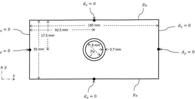
2-1 Boundary and loading conditions used in the numerical model of the

carotid artery. Arrows indicate a boundary condition applied to a specific point while curved lines without arrows indicate a boundary or loading condition applied along an entire surface. In this figure, d is the displacement, p is the pressure, x is in the horizontal direction, and

2-2 Mesh generation process used to discretize each computational model of the carotid artery. In (a), a uniform grid is generated; in (b), the elements overlapping with the artery and lumen are removed; in (c), the nodes on the inner surface are projected on the surface of the outer wall of the artery; in (d), the artery elements are added to the model; in (e) and (f), the domain is extended to fill the dimensions described

in Figure 2-1. . . . . 50

2-3 Screen captures of the Abaqus model used for Model 1. In (a), the geometry is displayed. In (b), a typical stress distribution is shown where the model is in the deformed configuration. In (c), a close up of

the stress distribution near the vessel is shown. The stress units are MPa. 51 2-4 Screen captures of the Abaqus model used for Model 2. In (a), the

geometry is displayed. In (b), a typical stress distribution is shown where the model is in the deformed configuration. In (c), a close up of the stress distribution near the vessel is shown. The stress units are MPa. 51 2-5 When the bone is added in the computational model, it is extended

throughout the entire bottom of the computational domain. ... 52

3-1 The plots demonstrate the correlation of the force sweep with the ultrasound data. In (a), the force sweep is displayed as a function of time. In (b), the force sweep is displayed as a function of LabView data number. In (c), the force sweep is displayed, after synchronization with

the ultrasound video, as a function of ultrasound frame number. . . . 55

3-2 The image shows the details of the segmentation algorithm. The red lines are a sample of the 100 equiangular radial lines used in the Star-Kalman algorithm. The white contour represents the contour estimated by the algorithm for this particular frame. The white star is the center

of m ass of the contour. . . . . 57

3-3 Segmentation results. The black line shows the size of the artery versus force over many cardiac cycles. The dotted blue line shows a fit to the peaks and represents the size of the artery at systole versus force. The dashed blue line shows a fit to the valleys and represents the size of the

artery at diastole versus force. . . . . 60

3-4 Visualization of the split of the optimization problem into two successive

optim izations. . . . . 61

3-5 The k-fold cross-validation algorithm work flow. . . . . 68

3-6 The process used to find the bone location in each ultrasound image.

In (a), a typical ultrasound image frame in the study is shown. In (b), the entropy filter has been applied and the image has been converted to gray scale. In (c), the image fill function has been applied. In (d), the image close function has been applied. In (e), the image has been

converted to black and white. . . . . 71

4-1 Photo of one of the oscillometric cuffs used in this work. After pressing

the start button on the device, it automatically inflates and deflates,

then it reports the blood pressure. . . . . 74

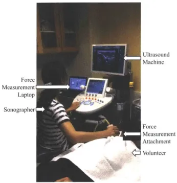
4-2 Orientation of the ultrasound system, sonographer, patient, and force

measurement laptop during data acquisition at MGH. . . . . 75

4-3 Photo of one of the ultrasound systems (GE Logiq E9) used in this

dissertation. The carotid artery is being imaged in the photo. .... 76

4-4 Screen capture of a typical ultrasound image obtained in the study at Massachusetts General Hospital. The ultrasound probe is pushing on the skin from the top surface of the image while the neck bone is

located at the bottom of the image. . . . . 77

4-5 The cartoon shows the approximate location of anatomical features

in the neck. In the orientation displayed here, the ultrasound probe is located next to the skin on the top surface of the cartoon. Typical

4-6 Screen capture of an ultrasound image in which the carotid artery is

imaged through its axis (i.e. longitudinally). . . . . 79

4-7 Solid modeling mock-up of the force measurement attachment used during this dissertation. The red clamp is attached to the blue outer clam shell through a load cell. Note that while the image shows a curved probe, only linear probes were used in this dissertation. The

device was developed by Dr. Matthew Gilbertson and Athena Huang. 80

4-8 The ultrasound force measurement attachment. The 3D-printed attach-ment is shown attached to a GE Logiq E9 linear 9L-D probe. In (a), the attachment is ready for use. In (b), the attachment is split apart so that the inner tight-fitting piece is visible. The device was developed

by Dr. Matthew Gilbertson and Athena Huang. . . . . 81

4-9 The LabView program used in order to record the applied force between the ultrasound probe and the tissue. The applied force is displayed in real time to the user. This program was designed by Dr. Matthew

Gilbertson and Athena Huang. . . . . 82

4-10 Screen capture of the LabView program in use. This program was

designed by Dr. Matthew Gilbertson and Athena Huang. . . . . 82

5-1 Raw algorithm results for the 24 healthy single-visit volunteers at MGH.

Each point represents one volunteer in the study. The plots (a)-(e) in

this figure are plotting the quantities described in Section 5.2. .... 86

5-2 Results on the test set after the k-fold cross-validation method is

applied to the 24 healthy volunteers at MGH. Each point represents one volunteer in the study. The plots (a)-(e) in this figure are plotting

the quantities described in Section 5.2. . . . . 87

5-3 Plots showing algorithm performance after applying the k-fold

param-eter set to the full set of 24 healthy volunteers at MGH. Each point represents one volunteer in the study. The plots (a)-(e) in this figure

are plotting the quantities described in Section 5.2. . . . . 88

5-4 Results of the real-time table lookup approach on 21 healthy single-visit volunteers. The k-fold parameters found previously in this chapter have been used to generate this plot. The plots (a)-(e) in this figure are

plotting the quantities described in Section 5.2. . . . . 90

5-5 Results of the technique after including the bone in the computational model. The results displayed are the raw results of the algorithm. The plots (a)-(e) in this figure are plotting the quantities described in

Section 5.2. . . . . 92

5-6 Results of the technique after including the bone in the computational model. The results displayed are the k-fold cross-validation results on the test set. The plots (a)-(e) in this figure are plotting the quantities

described in Section 5.2. . . . . 93

5-7 Results of the technique after including the bone in the computational model. The results displayed are the k-fold cross-validation parameter set applied to the full data set. The plots (a)-(e) in this figure are

plotting the quantities described in Section 5.2. . . . . 94

5-8 Intraobserver repeatability for systolic pressure (a) and diastolic pressure

(b ). . . . . 9 5

5-9 Condition number surface plot for one healthy volunteer in the study

at MGH. Four points are displayed in this figure. . . . . 96

5-10 Plot of the percent absolute relative error at systole and diastole versus

the artery thickness calculated by the optimization. . . . . 97

5-11 Absolute relative error corresponding to different force ranges. 'S' and 'D' refer to systolic and diastolic pressure. '1' refers to force range 1, which is from 2 N to 3 N. '2' refers to force range 2, which is from 2 N to 7.5 N. '3' refers to force range 3, which is from 2 N to 12 N. The

5-12 Absolute relative error corresponding to different force ranges. 'S' and 'D' refer to systolic and diastolic pressure. '1' refers to force range 1, which is from 2 N to 3 N. '2' refers to force range 2, which is from 2 N to 7.5 N. '3' refers to force range 3, which is from 2 N to 12 N. The results on four volunteers shown here are post-calibration data, where

the calibration was found in Section 5.3.2. . . . . 99

6-1 Cuff measurements versus time on a healthy volunteer. Measurements

were taken once every two minutes for 90 minutes. In (a), systolic and diastolic pressures versus time are displayed. In (b), the pulse rate is

displayed versus time . . . . 103

6-2 Results showing the variation of the algorithm measurements over a period of 90 minutes on healthy volunteer 1. The results presented here are raw algorithm results and did not undergo any post-processing cross-validation step. Part (a)-(e) show the quantities discussed in Section 5.2 and the plot in (f) shows the pressure versus minutes in the

study. ... ... 106

6-3 Results showing the variation of the algorithm measurements over a

period of 90 minutes on healthy volunteer 1. The results presented here are algorithm results in which the k-fold cross-validation algorithm has been applied and the resulting parameter set is applied to the test set. 107 6-4 Results showing the variation of the algorithm measurements over a

period of 90 minutes on healthy volunteer 1. The results presented here are algorithm results in which the k-fold cross-validation algorithm has been applied and the resulting parameter set is applied to the full set. 109 6-5 Results showing the variation of the algorithm measurements over a

period of minutes on healthy volunteer 2. The results presented here are raw algorithm results and did not undergo any post-processing

cross-validation step. Outliers were excluded from the plots. . . . . . 110

6-6 Results showing the variation of the algorithm measurements over a period of minutes on healthy volunteer 2. The results presented here are algorithm results in which the k-fold cross-validation algorithm has been applied and the resulting parameter set is applied to the test set.

Outliers were excluded from the plots. . . . .111

6-7 Results showing the variation of the algorithm measurements over a period of minutes on healthy volunteer 2. The results presented here are algorithm results in which the k-fold cross-validation algorithm has been applied and the resulting parameter set is applied to the full set.

Outliers were excluded from the plots. . . . . 112

6-8 The algorithm was applied to healthy volunteer 1 over 14 non-consecutive days. The figure shows the raw results of the algorithm before cross-validation. Part (a)-(e) show the quantities discussed in Section 5.2

and the plot in (f) shows the pressure versus day number . . . . 113

6-9 The algorithm applied to healthy volunteer 1 over 14 non-consecutive days. The results displayed here show the results after the k-fold cross-validation parameter set from healthy volunteer 1 in Section 6.3 (same volunteer as in this figure) was applied to the full set. Part (a)-(e) show the quantities discussed in Section 5.2 and the plot in (f) shows the

pressure versus day number. . . . . 114

6-10 The algorithm was applied to healthy volunteer 2 over 14 non-consecutive days. The figure shows the raw results of the algorithm before cross-validation. Part (a)-(e) show the quantities discussed in Section 5.2 and the plot in (f) shows the pressure versus day number. Outliers were

6-11 The algorithm applied to healthy volunteer 2 over 14 non-consecutive days. The results displayed here show the results after the k-fold cross-validation parameter set from healthy volunteer 2 in Section 6.3 (same volunteer as in this figure) was applied to the full set. Part (a)-(e) show the quantities discussed in Section 5.2 and the plot in (f) shows the

pressure versus day number. . . . . 116

6-12 Post-caffeine measurement minus pre-caffeine measurement for seven volunteers. Changes are displayed for algorithm systolic and diastolic pressures as well as oscillometric cuff systolic and diastolic pressure.

The algorithm results shown are the raw algorithm results. . . . . 118

6-13 Post-caffeine measurement minus pre-caffeine measurement for seven volunteers. Changes are displayed for algorithm systolic and diastolic pressures as well as oscillometric cuff systolic and diastolic pressure. The algorithm results are shown after the k-fold cross-validation parameter

set from healthy volunteer 1 in Section 6.4.2 is applied. . . . . 119

6-14 Post-exercise measurement minus pre-exercise measurement for four volunteers. Changes are displayed for algorithm systolic and diastolic pressures as well as oscillometric cuff systolic and diastolic pressure.

The algorithm results shown are the raw algorithm results. . . . . 120

6-15 Post-exercise measurement minus pre-exercise measurement for four volunteers. Changes are displayed for algorithm systolic and diastolic pressures as well as oscillometric cuff systolic and diastolic pressure. The algorithm results are shown after the k-fold cross-validation parameter

set from healthy volunteer 1 in Section 6.4.2 is applied. . . . . 121

6-16 Results on a healthy volunteer both before and after exercise. The results shown here are raw results of the optimization before any

cali-bration took place. . . . . 123

6-17 Results on a healthy volunteer both before and after exercise. For the results shown here, the k-fold cross validation parameter set from

healthy volunteer 1 in Section 6.3.2 was applied to the full data set. . 124

6-18 Results showing a compilation of most self-scans completed for the studies on healthy volunteers in this chapter. The results presented here are raw algorithm results. The figure plots the quantities discussed

in Section 5.2. . . . . 126

6-19 Results showing a compilation of most self-scans completed for the studies on healthy volunteers in this chapter. The results presented here are test set results from the k-fold cross-validation method. The

figure plots the quantities discussed in Section 5.2. . . . . 127

6-20 Results showing a compilation of most self-scans completed for the studies on healthy volunteers in this chapter. The results presented here are full data set results after the k-fold cross-validation parameter

set w as applied. . . . . 129

7-1 Algorithm results showing the variation of blood pressure readings on

a medicated hypertensive volunteer over the course of approximately 15 minutes. The results displayed here are the raw results of the algorithm without any post-processing. Plots (a) through (e) show the quantities discussed in Section 5.2; plot (f) shows the trend lines over

approximately 15 minutes for both cuff and algorithm. . . . . 133

7-2 Algorithm results showing the variation of blood pressure readings on

a medicated hypertensive volunteer over the course of approximately 15 minutes. The results displayed here are the test set results after the k-fold cross-validation algorithm was applied. Plots (a) through (e) show the quantities discussed in Section 5.2; plot (f) shows the trend

7-3 Algorithm results showing the variation of blood pressure readings over the course of approximately 15 minutes for the multi-visit medicated hypertensive volunteer. The results shown here are the results of the algorithm after the k-fold cross-validation parameter set is applied to the entire set. Plots (a) through (e) show the quantities discussed in Section 5.2; plot (f) shows the trend lines over approximately 15

minutes for both cuff and algorithm. . . . . 136

7-4 Algorithm results showing the variation of blood pressure readings on a hypotensive volunteer over the course of approximately 15 minutes. The results displayed here are the raw results of the algorithm without any post-processing. Plots (a) through (e) show the quantities discussed in Section 5.2; plot (f) shows the trend lines over approximately 15 minutes for both cuff and algorithm. Outliers were excluded from the

p lots. . . . . 13 7

7-5 Algorithm results showing the variation of blood pressure readings on a hypotensive volunteer over the course of approximately 15 minutes. The results displayed here are the test set results after the k-fold cross-validation algorithm was applied. Plots (a) through (e) show the quantities discussed in Section 5.2; plot (f) shows the trend lines over approximately 15 minutes for both cuff and algorithm. Outliers were

excluded from the plots. . . . . 138

7-6 Algorithm results showing the variation of blood pressure readings over the course of approximately 15 minutes for the multi-visit hypotensive volunteer. The results shown here are the results of the algorithm after the k-fold cross-validation parameter set is applied to the entire set. Plots (a) through (e) show the quantities discussed in Section 5.2; plot (f) shows the trend lines over approximately 15 minutes for both cuff

and algorithm. Outliers were excluded from the plots. . . . . 139

7-7 Algorithm results from the seven visits by a medicated hypertensive volunteer. The results shown here are the raw algorithm results. Plots (a) through (e) show the quantities discussed in Section 5.2; plot (f)

shows the trend lines over the 7 days for both cuff and algorithm. . . 140

7-8 Algorithm results from the seven visits by a medicated hypertensive volunteer. The results shown here were obtained by applying the k-fold cross-validation results from Section 7.2.1 to the full set. Plots (a) through (e) show the quantities discussed in Section 5.2; plot (f) shows

the trend lines over the 7 days for both cuff and algorithm. . . . . 141

7-9 Algorithm results from the 14 visits by a hypotensive volunteer. The results shown here are the raw algorithm results. Plots (a) through (e) show the quantities discussed in Section 5.2; plot (f) shows the trend lines over the 14 days for both cuff and algorithm. Outliers were

excluded from the plots. . . . . 143

7-10 Algorithm results from the 14 visits by a hypotensive volunteer. The results shown here were obtained by applying the k-fold cross-validation results from Section 7.2.2 to the full set. Plots (a) through (e) show the quantities discussed in Section 5.2; plot (f) shows the trend lines over the 14 days for both cuff and algorithm. Outliers were not excluded

from the plots. . . . . 144

7-11 Results from four single-visit older volunteers. The results displayed here are the raw results of the algorithm, before any post-processing procedures were completed. The plots in the figure show the quantities

7-12 Results from four single-visit older volunteers. Recall that two of these volunteers took data on the GE system and two took data on

the Supersonics system. The results displayed here are obtained by applying the k-fold parameter set from Section 6.4.2 on the two GE

system volunteers and the parameter set from Section 5.3.2 on the two Supersonics volunteers. The plots in the figure show the quantities

discussed in Section 5.2 . . . . . . . . . 147

8-1 Rendering of a proposed device that uses the technique described in

this dissertation. . . . . 153

List of Tables

1.1 Summary of blood pressure estimation techniques . . . . 37

3.1 The initial parameter values for the first optimization . . . . 66

3.2 The initial parameter values for the second optimization. . . . . 66

3.3 Sample portion of the look-up table used during the real-time

optimiza-tion approach. The results displayed here are the raw algorithm results,

before any calibration procedures were completed. . . . . 69

5.1 Statistics obtained after running the k-fold cross-validation method for

2000 different random sortings into training set and test set. The results here correspond to the 24 healthy single-visit volunteers at MGH. In this table, a is a 2000 element vector where each element of the vector

is the mean of the errors in a particular random sorting. . . . . 89

5.2 Statistics obtained after running the k-fold cross-validation method for

all sortings into training set and test set. The results shown are those in which the bone was included in the computational model. In this table, a is a vector where each element of the vector is the mean of the

6.1 Statistics obtained after running the k-fold cross-validation method for 2000 different random sortings into training set and test set. The table shows the results from healthy volunteer 1 who had measurements taken many times of a period of 90 minutes. In this table, a is a 2000 element vector where each element of the vector is the mean of the

errors in a particular random sorting. . . . . 108

6.2 Statistics obtained after running the k-fold cross-validation method

for 2000 different random sortings into training set and test set. The results are from a compilation of self-scans on healthy volunteers. In this table, a is a 2000 element vector where each element of the vector

is the mean of the errors in a particular random sorting. . . . . 128

7.1 Statistics obtained after running the k-fold cross-validation method for

all sortings into training set and test set for the multi-visit medicated hypertensive volunteer. In this table, a is a vector where each element

of the vector is the mean of the errors in a particular random sorting. 135

Chapter 1

Introduction

Blood pressure is an important physiological parameter commonly measured both

by medical professionals in a clinical environment

[4,5]

in a home environment

[5].

an indication of the health of a patient. Complications of high blood pressure, also known as hypertension, include stroke, renal failure, peripheral vascular disease, and heart disease, among many other diseases [4-6]. Thus, it is important that there is an easy-to-use and accurate blood pressure measurement technique available.

1.1

Blood Pressure Basics

The heart pumps blood through the arteries to the body's periphery and the blood returns to the heart through the veins. Due to the pumping nature of the heart, the blood pressure in arteries cycles between a maximum, termed systolic blood pressure, and a minimum, termed diastolic blood pressure. A typical healthy patient has a systolic pressure of about 120 mmHg and a diastolic pressure of about 80 mmHg (1 mmHg is equivalent to approximately 133.3 Pa). The fluctuation of pressure in the arteries takes a characteristic shape as shown in Figure 1-1. The difference between systolic pressure and diastolic pressure is termed the pulse pressure. The mean arterial pressure can be found by taking an average over a period of the curve in the figure. An approximate, back-of-the-envelope, formula used to calculate mean arterial pressure is

150 140- 130-120 110 - 100- 90-80 70 60 0 0.5 1 1.5 2 2.5 Time (s)

Figure 1-1: Typical blood pressure versus time trace in arteries [1-3]. The maximums

are termed systolic pressure and the minimums are termed diastolic pressure.

Pma 1 2

P ~-Ps + -Pd (1.1)

3 3

where Pma is the mean arterial pressure, P, is the systolic pressure, and Pd is the

diastolic pressure. The blood pressure in the aorta is termed 'central blood pressure' [7]. Central blood pressure has been shown to be more closely related to intermediate

cardiovascular risks than the blood pressure in the brachial artery [7].

It has been reported that while diastolic and mean arterial pressure are mostly constant throughout the arterial tree, the systolic pressure is often greater in the

periphery than in the aorta [8]; this is due to the fact that as the blood moves from the

aorta to the periphery, the arteries become stiffer and less elastic [8]. In one study, it was reported that systolic pressure in the radial artery is 112% of the central systolic

pressure _[9].

Blood pressure can change rapidly, which makes it difficult to validate blood

pressure measurement techniques. In one paper, it was reported that blood pressure can change by as much as 20 mmHg over the course of 'a few heart beats' [5,101.

1.2

Desirable Characteristics of a New Blood

Pres-sure MeaPres-surement Device

The desirable characteristics of a new blood pressure measurement device include being usable in a variety of everyday situations, e.g. in-the-home, hospital, and even on-the-go. It would be advantageous if the device would be non-invasive and non-occlusive (i.e. it would not cut off blood flow to any area of the body). Providing accurate and continuous blood pressure readings without any calibration would be beneficial as well.

It would be helpful for the results of the device to be displayed to the user immediately and also recorded for future processing and trend identification. Further, wireless connection to various electronic devices would also be helpful. Finally, it would be great if the data was sharable with an appropriate medical professional whenever needed.

1.3

Blood Pressure Measurement Techniques

There are no existing blood pressure measurement techniques that meet the specifica-tions of the blood pressure measurement device outlined above. Below, the existing blood pressure measurement techniques are described. A summary is included in Table 1.1.

1.3.1

Arterial Catheter

The invasive arterial catheter, inserted most commonly at the radial artery near the wrist, gives a direct blood pressure measurement [11]. While the invasive catheter can be used on most patients, it is not used on patients with Raynaud's phenomenon, thromboangiitis obliterans, infection near the insertion site, or traumatic injury near the insertion site [12]. Since the procedure is invasive, the procedure does have risks, including permanent ischaemic damage (0.09 %), temporary occlusion (19.8%), sepsis (0.13%), local infection (0.72%), pseudoaneurysm (0.09%), haematoma (14.4%), and

bleeding (0.53%) [11]. Further risks [11] include abscess, cellulitis, paralysis of the median nerve, suppurative thrombarteritis, air embolism, compartment syndrome, and carpal tunnel syndrome. While the risk percentages of these complications are reported to be very low, the invasive nature of the procedure makes it impractical outside of a hospital. Further, when a catheter is used at the radial artery, it can only measure blood pressure in the periphery, which is different than central blood pressure in the aorta, as discussed in Section 1.1.

1.3.2

Auscultatory Cuff

The blood pressure cuff, also known as a sphygmomanometer, is a common device used for blood pressure estimation [4]. Many different blood pressure measurement methods rely on the cuff. The manual auscultatory method is a cuff-based method used by medical professionals. In the manual auscultatory method, after inflating the cuff and while decreasing cuff pressure, the doctor listens to blood flow sounds using a stethoscope. The doctor makes a judgment on systolic and diastolic pressures using the Korotkoff sounds, defined as the typical sounds blood makes as the cuff decreases

in pressure [4]. The first Korotkoff sound occurs when sound is initially audible and

corresponds to the systolic pressure; the fifth Korotkoff sound occurs when the blood flow sounds disappear and corresponds approximately to the diastolic pressure [4]. While popular, the blood pressure cuff cuts off blood flow to the arm and thus is not suitable for continuous blood pressure estimation. Further, the auscultatory method requires a trained professional in order to obtain a reading, and thus the method cannot be used in-the-home or on-the-go. Elevated readings are also common due to the white-coat effect [13].

Mercury-based Sphygmomanometer

Mercury-based sphygmomanometers use the auscultatory method described above. However, in this application, a column of mercury is used to indicate the cuff pressure. While this device has, in the past, been labeled the gold standard for non-invasive

blood pressure measurement, it has been phased out by the medical community due to the dangers of mercury [4].

The literature has reported that mercury-based auscultatory methods over predict both systolic and diastolic blood pressure compared to invasive catheters [14]. In [14], the systolic pressure correlation was 0.84 and the diastolic pressure correlation was 0.59 compared to invasive catheters. However, in another paper, it was reported that there is no statistically significant difference between mercury auscultatory cuff

measurements and invasive arterial line measurements when the patient is at rest

[15].

Aneroid Sphygmomanometer

Aneroid sphygmomanometers also use the auscultatory method described above. However, in this application, the cuff pressure is increased by repeatedly squeezing a mechanical 'balloon' and the cuff pressure is displayed on a circular gauge for the doctor to use. Because there are many moving parts, such devices are highly sensitive to poor treatment of the device, e.g. accidentally dropping the device or hitting the device on the side of a table [4].

Devices are reported to vary greatly in accuracy depending on the manufacturer

[4].

In one study, it was reported that 44% were inaccurate in a hospital setting [16]. However, in a study of only the Welch Allyn Tycos 767-Series mobile aneroid device (Welch Allyn, Skaneateles Falls, New York, USA), it was reported that there is no statistically significant difference between aneroid and mercury measurements for systolic pressure and only a small statistically significant difference for diastolic pressure [17].

Hybrid Sphygmomanometer

Hybrid sphygomanometers use the auscultatory method and combine the features of the mercury-based devices and the aneroid devices. In particular, the display is often fully digital, allowing for both pressure readings and pulse rate to be displayed.

One study evaluates the validity of the Nissei DM3000 hybrid device (Japan Precision Instruments Inc., Gunma, Japan) and shows that it has the same level of

accuracy as the mercury-based sphygmomanometer discussed above [181. Another study examined the A&D UM-101 device (A&D Company Limited, Tokyo, Japan) and concluded that one version of the device passes the European Society of Hypertension

International Protocol for validation of blood pressure measurement devices

[191.

1.3.3

Oscillometric Cuff

Automatic blood pressure cuffs are available for use in-the-home or in a hospital setting and use the oscillometric method [4]. In the oscillometric method, the cuff is first placed on the upper arm of the user. After the start button is pressed, the cuff

inflates automatically and, as it is deflating, cuff pressure oscillations are sensed

[4].

From the envelope of the recorded cuff pressure oscillations, systolic, diastolic, and mean arterial pressure can be approximated using various methods [5]. For example, the maximum amplitude algorithm identifies the cuff pressure at which the envelope reaches a maximum as the mean arterial pressure and identifies systolic and diastolic pressures as the cuff pressure at which the envelope reaches certain fractions of the maximum; many other techniques have been developed, including using derivatives of

the envelope or neural networks

[15].

find systolic and diastolic pressures are proprietary

[4].

It has been reported that different cuffs give different readings for blood pressure and that mean arterial pressure is typically underestimated by oscillometric blood

pressure cuffs

[4].

children, pregnant women, and patients with atrial fibrillation [20]. Furthermore, the literature recommends that oscillometric measurements are separated by at least one minute and that the average of three readings are taken as the patient's blood pressure [4]. The method occludes the artery and is uncomfortable for patients. Oscillometric cuffs can be obtained at drugstores for between $15-$50.

It has been reported that the agreement between oscillometric blood pressure cuffs

and invasive pressure measurements is -6.7 9.7 mmHg (p<.0001)

[21].

26.4% of measurements had a discrepancy, compared to the catheter, between 10 mmHg and 20 mmHg while 34.2% had a discrepancy of at least 20 mmHg [21].

Finger Oscillometric Method

The oscillometric method described above for upper arm measurements has been applied to cuffs placed around the finger. However, it has been reported that such devices suffer from significant variability issues and, thus, are not to be used [22].

Wrist Oscillometric Method

The oscilometric method described above has also been extended to apply to the wrist. The advantage of taking blood pressure using a wrist cuff is that wrist size does not vary much in obese patients. One author has reported that wrist cuffs have potential for widespread use [4].

1.3.4

Tonometry

Tonometry, also known as applanation tonometry, is a blood pressure measurement technique originally developed for use at the wrist. In the method, a pressure transducer is placed next to an artery supported by a bone and the transducer readings are assumed to be related to the blood pressure within the artery [4]. Tonometry is a medical term meaning 'to measure pressure' and applanation is a medical term meaning 'to flatten' [23]. Using system models (e.g. transfer functions), tonometry can be used to estimate central blood pressure [24].

The accuracy and precision of tonometry, compared with invasive pressure

mea-surements, has been reported as -5.8 14.2 mmHg for systolic pressure, 7.2 8.3

mmHg for diastolic pressure, and 3.9 8.8 mmHg for mean arterial pressure [25].

One advantage of tonometry is that the entire pressure waveform can be obtained with the technique; however, the method requires calibration with an external device such as a cuff [24]. Tonometry is also very sensitive to placement of the device [26].

1.3.5

Photoplethysmography Methods

A plethysmograph is an instrument used to estimate the volume or volume change of an organ. In photoplethysmography (PPG), the volume of the artery is usually

obtained using a device called a pulse oximeter, which is placed on the finger. As blood pulses through the finger, the amount of light transmitted and reflected changes. In pulse oximetry, light transmission or reflection is measured, which is related to the amount of blood in the artery and thus to the volume of the artery. A PPG graph shows the relation between amplitude of the signal in volts versus time. This information has been used in many different ways, with and without calibration, to estimate absolute blood pressure; the literature does not appear to focus significantly on using PPG to measure relative pressure changes. In the following sub-sections, various PPG-based techniques are discussed and the calibration details of each method is described.

Photoplethysmography Alone

A PPG signal alone can be used to estimate relative blood pressure. There are different approaches taken in the literature to obtain blood pressure from only a PPG signal, but all techniques use a calibration step that relates certain features of the PPG reading to blood pressure. The calibration step is needed because the PPG signal itself does not give enough information to find blood pressure; it is not an estimate of blood pressure by itself. The calibration step can be completed using many different approaches. In one approach, the features are extracted directly from a PPG recording taken at the periphery and a regression equation relates the parameters to blood pressure [27,28]. In another approach, a pulse wave analysis algorithm is used to extract features, then a regression or calibration step is completed to obtain a blood pressure reading [29].

Pulse Transit Time

The pulse transit time has been related to the pressure within an artery. Specifically, the pulse wave velocity, V, is defined for elastic arteries as [30]

V = t (1.2)

2 Rp

where E is the elastic modulus of the artery, t is the artery thickness, R is the inner artery radius, and p is the density of the blood.

The literature states that pulse wave velocity can be found as

[301

V = D (1.3)

t

where D is the distance between the aorta and the location in the periphery where data is collected, and t is the pulse transit time, i.e. the time it takes for a pressure pulse to travel from the aorta to the periphery where data is collected. In order to calculate D, researchers use the height of the patient multiplied by a constant factor. To calculate t, researchers estimate the time between the R-wave of an electrocardiogram (ECG) and the peak of the PPG signal obtained at the periphery [31].

In order to relate pulse wave velocity to the blood pressure, the literature investi-gates many different models. For example, one author [30] relates the artery elasticity to the pressure using the equation

E = Eoe(P-PO) (1.4)

where E0, Po, and a are parameters to be determined and P is the pressure. Another

author [32] derives the equation

S_(0.6hi)2_p

P = _1.4t2. 2 + pgh2 (1.5)

where g is the acceleration due to gravity, h, is the height of the patient, and h2 is

the height difference between acquisition locations.

This method requires access to both an ECG and a time correlated PPG. However,

the method has been shown to compare favorably to cuff measurements

[32].

Some pulse wave velocity methods require calibration while others are calibration-free [30,33]. In either case, the unknown parameters in Equation 1.4 need to be considered [33]. In one calibration method, a single oscillometric cuff measurement is used in addition to the known pressure change that occurs when raising the hand

(i.e. hydrostatic pressure change) [33]. In a calibration-free method, features of the PPG signal and ECG are used with machine learning of a large database to find the parameters [30].

Finger Cuff

In another PPG-based blood pressure measurement technique, a finger cuff is used to record the PPG signal; this method is alternatively referred to as the vascular unloading technique. As the PPG is recorded, the cuff automatically inflates or deflates in order to keep the blood volume in the finger constant. The pressure required to keep blood volume constant is related to the blood pressure within the vessel [4,34]. This is called the Penaz method and was first introduced in 1973 [35]; the method was used in the Finapres finger cuff device. While this method has been shown to give accurate estimates of pressure changes, one author suggests that it is not clinically used because of its cost, inconvenience, and high degree of variability when measuring absolute values of pressure [36].

1.3.6

Other Techniques

Other techniques are being developed by research groups to estimate arterial blood pressure non-invasively and potentially continuously using the behavior of ultrasound contrast agents in the blood stream [37-39]. By investigating cavitation frequency, radial oscillations, and general microbubble behavior, blood pressure can be estimated [37]. It has been reported that accuracy might be low with some variations of this technique [37] and it is clear that injection of microbubbles would not be ideal in every circumstance.

In a different technique related to ours, ultrasound and image processing methods are used to measure non-invasively central venous pressure [40]. By tracking the deformation of a superficial vein in the forearm due to an externally applied force, the group estimates the absolute pressure at which the vein will collapse. The collapsing pressure is taken to be the central venous pressure.

Table 1.1: Summary of blood pressure estimation techniques

Method Description Advantages Disadvantages

-Terminal digit preference [41

-Inter-observer error [41]

Auscultatory blood Doctor listens to Korotkoff sounds [4 -Comparable to mercury -White coat effect if physician takes measurement [4]

pressure cuff (Hybrid Method) sphygmomanometer [41] -Errors occur due to improper rate of deflation [42,43]

-Time consuming [41]

-Optimal cuff size and placement required [41] -Under- or over- estimation compared to brachial Cuff automatically inflates and deflates -Gives accurate estimate of pressure changes [4] pressure measurements [4]

Finger cuffs to keep blood volume constant [34,44] h Allows ambulatory measurement over 24 -Cost, inconvenience, and inaccuracy when measuring

absolute pressures [4] -Invasive

Invasive arterial Pressure transducer placed inside artery [11] -Reliable and accurate; considered gold standard -Risk of hemorrhage, infection, thrombosis, ischemia,

line by some [41,45] hematoma, accidental injection of intravenous drugs,

neuronal or adjacent structure injury [41,45] -Requires an injection of microbubbles into blood

-Non-invasive [46] stream [46]

Microbubbles Response of microbubbles to ultrasound [37] -Potentially applicable to all chambers of -Requires ultrasound [46]

heart [46 -Some methods reported either low reliability, poor

absolute pressure value compared to pressure changes, and low resolution [37]

-Confounding factors relate to the shape and amplitude of the oscillometric envelope and include

-No transducer needed above artery so artery stiffness [4,20]

placement is not critical [4] -Poor accuracy when used on children, pregnant

Oscillometric blood pressure cuff Automatic cuff processes pressure changes as -Less susceptible to external noise [4] women, and patients with atrial fibrillation [20]

cuff deflates [47] -For ambulatory monitoring, cuff can be -Many algorithms are proprietary [4,20]

removed and replaced by patient [4] -Different devices give different readings [4,20]

-Cheap and ubiquitous [20,41] -Do not work well during physical activity [4]

-Many devices have not been validated against published standards [20]

Proposed method Uses finite element analysis to solve the blood - Nn vse -Requires ultrasound probe

pressure inverse prbe_ Non-occlusive

pressure iverse problem - No calibration needed - Requires a 3D printed force measurement attachment

-When used at radial artery, it is a better -Requires calibration for each patient [4] estimate of central arterial pressure than finger cuffs [41 -Not suitable for routine clinical use [4]

Gauge measures force variation on skin -Less sensitive than finger cuffs to - Not sit or re in e [4

Tonometry surface [26] vasoconstriction and vascular disease [41] -Some variations are position dependent [4,41]

-Agreement with arterial line in some (but -Not reliable for elderly patients or for rapid and

not all) studies [41] large changes in blood pressure [41]

-Non-invasive [48] _{Technique has only been applied to superficial}

Vessel collapse Computer vision techniques predict point of -Easy for non-experts [48] veins [48]

collapse of superficial vein [48] -Automatic readings [48]

1.4

Relevant Patents

At least three patents have been awarded which briefly mention the measurement of blood pressure using artery displacements, which are often visualized using ultrasound

[49-51]. This is relevant because the method discussed in this dissertation relies on

artery deformations to calculate blood pressure. In all of these patents, the absolute blood pressure is obtained using a reference or calibration point provided by the operator, often from a separate device such as a cuff.

In a separate, patented method of non-invasive and potentially continuous blood pressure estimation [52], two blood pressure cuffs are used together; one cuff provides a periodic calibration, and the other cuff provides the change in pressure from the calibration point.

There is also a non-invasive, continuous blood pressure estimation patent that relies on pulse wave velocity methods and that implements an automatic calibration technique [53].

1.5

Accuracy Requirements of New Blood Pressure

Measurement Techniques

There are a number of different standards that can be used to validate new blood pressure measurement techniques, with some validation standards specific to sphyg-momanometers [4,54, 55]. It is important to note that, from a regulatory perspective, it is optional for manufacturers to meet published validation standards; in fact, there are many oscillometric cuffs on the market that do not meet published standards.

The European Society of Hypertension International Protocol, published in 2010, compares new blood pressure measurement techniques to two mercury auscultatory cuffs [54]. An additional standard, specific to ambulatory monitoring, published by the British Hypertension Society in 1990, also uses the mercury auscultatory cuff as the gold standard [56].

1.6

Clinical Need

Clinically, doctors choose between three non-ideal techniques to measure blood pressure: an invasive arterial catheter, an oscillometric blood pressure cuff, or an auscultatory cuff. Even though the catheter gives continuous and accurate data, inserting the catheter is an invasive procedure. The oscillometric cuff cannot give pressure mea-surements continuously because it occludes the artery and it has been shown to

significantly underestimate mean arterial pressure in patients with atherosclerosis

[4].

The auscultatory cuff not only occludes the artery but also requires valuable time from medical professionals. Thus, there is a need for a blood pressure measurement device that serves as an intermediate option between the invasive catheter and cuff techniques. One contribution of the dissertation is a proof-of-concept of a new, intermediate option between catheter and cuff.

1.7

Previous Related Work

In this dissertation, a novel approach using ultrasound is taken to address the clinical arterial blood pressure measurement need described above. Our inspiration to use ultrasound to non-invasively measure arterial blood pressure is quantitative ultrasound elastography, which is a well-known method that uses ultrasound to measure tissue stiffness, i.e. elastic modulus; a review of various elastography methods has been published [57].

The application of elastography methods to blood pressure estimation was first discussed by the author in 2012. Simulated data were used in highly simplified scenarios to estimate pulse pressure [58]. Pulse pressure was included as a variable along with elastic modulus in an elastography inverse problem. The pulse pressure algorithms were confirmed using phantom experiments in [59]. In our paper, we suggested that a new methodology was needed in order to estimate the mean arterial pressure component of the cardiac cycle [60]. This dissertation details a new methodology that accomplishes that goal.