Treegrass: a 3D, process-based model for simulating plant
interactions in tree – grass ecosystems
G. Simioni
a,*, X. Le Roux
b, J. Gignoux
a, H. Sinoquet
baLaboratoire Fonctionnement et E6olution des Syste`mes Ecologiques, Uni6ersite´ Paris
6-CNRS-ENS,46 rue d’Ulm,
75230 Paris, Cedex 05, France
bU.A. Bioclimatologie-PIAF (INRA Uni6ersite´ Blaise Pascal), Site de Crouelle,234 A6enue du Bre´zet,
63039 Clermont-Ferrand Cedex 02, France
Received 15 September 1999; received in revised form 21 February 2000; accepted 21 February 2000
Abstract
The function and dynamics of savanna ecosystems result from complex interactions and feedbacks between grasses and trees, involving numerous processes (i.e. competition for light, water and nutrients, fire, and herbivory). These interactions are characterised by strong relationships between vegetation structure and function. Given the heteroge-neous structure of savannas, modelling appears as a convenient approach to study tree – grass interactions. Most current models that describe carbon and water fluxes are not spatially explicit, which restricts their ability to simulate plant interactions at small scales in heterogeneous ecosystems. We present here a new 3D process-based model called TREEGRASS. The model aims at predicting, in heterogeneous tree – grass systems, plant individual radiation, carbon and water fluxes at a local spatial scale. It is run at a daily time-step over periods ranging from one to a few years. The model includes (i) a 3D mechanistic submodel simulating radiation and energy (i.e. transpiration) budgets; (ii) a soil water balance submodel, and (iii) a physiologically based submodel of primary production and leaf area development. The ability of TREEGRASS to predict the seasonal courses of grass dead and leaf mass, soil water content and light regime as observed in the field has been tested for grassy and shrubby areas of Lamto savannas (Ivory Coast). Simulations showed that the spatial distribution of primary production can be strongly affected by the spatial vegetation structure. Potential applications involve predicting net primary production and water balance from the individual to the ecosystem and from the day to the annual vegetation cycle (e.g. effects of tree spatial patterns on carbon and water fluxes at the ecosystem level). © 2000 Elsevier Science B.V. All rights reserved.
Keywords:Savanna; Spatial patterns; Primary production; Water balance; Radiation absorption; Simulations
www.elsevier.com/locate/ecolmodel
1. Introduction
Savannas are defined as ecosystems where a continuous grass layer and a discontinuous tree layer coexist (Scholes and Archer, 1997). Savanna ecosystems cover about 20% of continental sur-* Corresponding author. Tel.: + 44323706; fax +
33-1-44323885.
E-mail address:[email protected] (G. Simioni).
0304-3800/00/$ - see front matter © 2000 Elsevier Science B.V. All rights reserved. PII: S 0 3 0 4 - 3 8 0 0 ( 0 0 ) 0 0 2 4 3 - X
faces (Scholes and Hall, 1996) and 40% of tropical land surfaces (Solbrig et al., 1990). In addition to their highly heterogeneous vegetation structure, these ecosystems are characterised by complex interactions between tree and grass individuals that compete for light, water and nutrient re-sources. Being able to predict grass and tree func-tioning separately does not enable to predict the functioning of the coupled tree – grass system. This restricts our ability to predict tree – grass stability and dynamics in savannas (Scholes and Archer, 1997).
Assessment of tree – grass interactions has mainly been addressed by field studies. Most of them have focused on the effects of trees on the biomass and primary production of the grass layer (e.g. Knoop and Walker, 1985; Stuart-Hill and Tainton, 1989; Weltzin and Coughenour, 1990; Belsky, 1994; Mordelet and Menaut, 1995), on the soil water balance (e.g. Knoop and Walker, 1985; Joffre and Rambal, 1988; Mordelet, 1993a; Le Roux and Bariac, 1998) or on soil nutrient availability (e.g. Isichei and Muoghalu, 1992; Mordelet et al., 1993; Cruz, 1997; Rhoades, 1997). Though necessary, these studies do not point out the different processes that determine the integrated effect of one vegeta-tion component on the other, but rather appear as a list of particular case studies.
Thus, for some authors, the only way to gain a comprehensive understanding of tree – grass coex-istence and to account for the effect of vegetation structure on ecosystem physiology is to build specific models (Jeltsch et al., 1996; Scholes and Archer, 1997). During the last two decades, sev-eral modelling approaches have been proposed to simulate the functioning of tree – grass systems (Scholes and Archer, 1997). Some authors have developed models of tree – grass equilibrium that focused on the competition for soil water (Walker et al., 1981; Eagleson and Segarra, 1985). These models were generally based on a spatial segrega-tion between grass roots exploiting mainly surface soil layers, and tree roots exploiting mainly deeper layers. More recently, simulation models predict-ing the effects of tree – grass interactions on grass and tree production have been developed. Among them, the GRASP model (Littleboy and McKeon,
1997) represents competition for water and nutri-ents, and the CENTURY-Savanna model (Parton and Scholes, unpublished), a tree – grass version of CENTURY (Parton, 1996), is based on competi-tion for nutrients. These two models were de-signed to compute the bulk functioning of the tree and grass components of tree – grass systems, and use bulk information on vegetation structure (i.e. tree leaf and root biomasses or tree basal area computed at site scale) to drive tree – grass compe-tition. The SAVANNA model (Coughenour, 1994) is a process-based model that is spatially explicit at the landscape scale (i.e. it is not individ-ual based but each pixel is an association of one tree – grass zone and one pure grass zone). How-ever, the choice of a relevant variable to define the respective size and dynamics of these two areas is still unclear (Coughenour, pers. comm.). To our knowledge, the only savanna model that accounts for tree individual spatial structure is the automa-ton model of Jeltsch et al. (1996). This model is suitable for predicting the effects of natural or man induced disturbances on tree dynamics and tree – grass equilibrium, but was not designed to study the effect of vegetation structure on water or carbon fluxes in savannas. Other modelling studies have emphasized the importance of spatial patterns (Korzukhin and Ter-Mikaelian, 1996; Pacala and Deutschman, 1995; Weishampel and Urban, 1996).
In this paper, we present a simulation model, named TREEGRASS, designed to test the effects of the fine scale vegetation structure (i.e. tree density, tree spatial distribution, crown shape and crown size distribution) on tree – grass interactions (i.e. water and carbon budgets at the site level). TREEGRASS takes into account competition for light and water in a mechanistic and spatially explicit way, and uses a biologically based ap-proach to compute net primary production. The model is derived from three existing models: (1) the 3D RATP model (Radiation Absorption, Transpiration and Photosynthesis) (Sinoquet et al., 2000) that computes radiation and energy budgets within vegetation canopies; (2) the PEP-SEE model (Production Efficiency and Phenology in Savanna EcosystEms) (Le Roux et al., 1996) that simulates primary production and soil water
balance; (3) the MUSE simulation framework (MUltistrata Spatially Explicit model) (Gignoux et al., 1996) designed to represent an ecosystem as a set of individuals and their geometric features by a spatially explicit approach. In the next sec-tion, the TREEGRASS model is presented and is parameterised for a humid savanna ecosystem (Lamto, Ivory Coast). The ability of the model to simulate radiation absorption, primary produc-tion and soil water balance in pure grass and tree – grass areas is tested against field data. Limi-tations and possible applications of TREE-GRASS are discussed.
2. The TREEGRASS model
The main original features of the 3D TREE-GRASS model are that (1) trees are represented individually, (2) radial extensions of tree foliage and roots are taken into account, (3) the foliage and the root system are distributed into a grid of 3D cells, and (4) competition for light and water are treated mechanistically (i.e. most relationships used are biophysical).
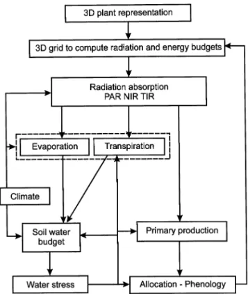
This model runs with a hourly/daily time step over one or a few vegetation cycles. The model has been developed in Borland Pascal 7. Processes considered in the model are presented in Fig. 1.
2.1. Main assumptions
The present version of TREEGRASS uses five major hypotheses:
1. Net primary production (NPP) is computed by the light use efficiency (LUE) approach (Mon-teith, 1972, 1977): one value for maximum LUE is used for trees and another value for grasses, while the same value is used for all the individuals on a site (maximum LUE values have to be determined from field measure-ments). The actual LUE is modulated by wa-ter stress. The assumption of the constancy of maximum LUE under different light regimes has recently been supported by the conceptual physiological model of Dewar et al. (1998). 2. The ratio of produced dry matter allocated to
roots to the amount allocated to shoots is computed as a function of actual to maximum LUE values (Landsberg and Waring, 1997). 3. Over one vegetation cycle, tree architecture
(crown volume and shape) is constant, and only the leaf area density (LAD) can change, tree dynamics and seedling growth are not implemented.
4. Rainfall interception by the foliage is neglected.
5. Climatic variables (wind, air temperature and humidity) are assumed to be spatially homoge-neous on the site.
Nutrients, in particular nitrogen, can play an important role in tree – grass interactions (see Bel-sky, 1994; Scholes and Archer, 1997), but they are not explicitly treated in TREEGRASS. The present model must be considered as a first ver-sion to which a soil organic matter submodel can be coupled, in order to include the nitrogen cycle. Two additional hypotheses were made for the simulations presented in this paper:
1. for a given simulation, only one species of grass and one species of tree are considered; Fig. 1. Processes computed in the TREEGRASS model.
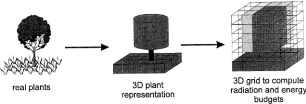
Fig. 2. Spatial representation of plants in TREEGRASS. The second picture shows the simple plant structural features used to represent trees (i.e. simple cylindrical crown, crown radius, and total height and bole height) and grasses (grass individuals are lumped into homogeneous plots and they form a continuous layer). Though they do not appear on this figure, roots are represented in a similar way. The third picture represents the 3D grid used to compute the spatial distribution of plant foliage as used by the radiation/energy budget submodel (different levels of grey correspond to different values of leaf area density (LAD)). Tree LAD is distributed using overlap coefficients between tree crown and cell volumes.
2. night transpiration is neglected (because of dew occurrence at night at the study site (Le Roux, 1995).
2.2. Spatial representation of the6egetation Plants are distributed within a 3D grid of cells (Fig. 2). The grid is divided into an above ground part, where the foliage is distributed into
6eg-etation cells, and a below ground part where roots
are distributed into soil cells. One vegetation cell can contain different types of leaves (green or dead, grass or tree, individual i or j ). In each cell, each leaf type is characterised by its LAD, in-clination distribution and optical properties. Soil cells can contain roots of different plants as well.
A grass individual occupies one above ground cell and the soil cells underneath. Tree foliage and root crowns are assumed to have cylindrical shapes. Trunks and branches are not explicitly represented. Tree leaves and roots are spread into vegetation and soil cells according to over-lap coefficients between cylinders and cells. Two grass ‘individuals’ (i.e. plots) do not share any vegetation nor soil cell, which is in accor-dance with the spatial distribution of roots ob-served for grasses in humid savannas (Le Provost, 1993). In contrast, a tree can share cells with grasses or with other trees. In particular, a tree compulsorily shares soil cells with grass indi-viduals.
2.3. Radiation absorption
The radiation submodel has been adapted from the RATP model (Sinoquet et al., 2000). Rays from several directions are directed into the cell grid. When a ray passes through a cell, it is attenuated following Beer’s law, depending on the LAD and on the angular distribution of the vege-tation entities (i.e. types of leaves) present in the cell. Intercepted radiation is shared between these entities, assuming that the leaves are randomly and uniformly distributed. Light interception by twigs and branches is neglected.
Radiation interception computed for each ray is used to calculate exchange coefficients between sources and receptors. Sky, foliage and soil are both sources (respectively of direct and diffuse radiation, and of transmitted or reflected radia-tion) and receptors. For one day, five representa-tive sun directions are computed (corresponding to daytime 6:00, 9:00, 12:00, 15:00 and 18:00 h). These directions vary with the day of year and latitude. For diffuse and reflected radiation, the direction space is divided into solid angles, centered around representative heights and azimuths. Incident dif-fuse radiation is calculated assuming a standard overcast sky luminance distribution (Moon and Spencer, 1942). Sources of reflected radiation are calculated considering that reflection and transmis-sion are isotropic and depend only on the angular distribution of organs. Exchange coefficients be-tween a source and a receptor are built in
a progressive manner, adding the contribution of beams coming from the source when they meet the receptor.
These exchange coefficients are first calculated for diffuse and scattered radiation (depending thus only on the foliage characteristics and on the sky luminance distribution). For direct radiation, ad-ditional exchange coefficients are then computed for each time step, i.e. each sun direction. The first step is necessary only when the LAD of one individual has undergone a significant change. Hence, to save calculation time, exchange coeffi-cients are computed only when a significant change in LAD (20% in our simulations) of at least one individual has occurred.
Radiation fluxes intercepted by each entity in each cell are computed by using the radiosity method (Ozisik, 1981): the flux intercepted by a given receptor is a linear combination of fluxes coming from the whole set of sources weighed by the exchange coefficients between the sources and the receptor. Intercepted fluxes (including multiple scattering) are thus written as a system of linear equations. Solving this system allows us to calcu-late radiation fluxes. Details on the calculation can be found in Sinoquet and Bonhomme (1992) and in Sinoquet et al. (2000).
2.4. Transpiration and e6aporation
Energy budget is computed in three dimensions to determine, for each entity in each cell, the organ temperature that balances fluxes of received and lost heat:
Rnjk− Hjk− Ejk= 0 (1)
where Rnjkis the net radiation absorbed by entity
j in cell k, and Hjkand Ejk are sensible and latent
heat fluxes lost by entity j in cell k. Energy bud-gets are established for shaded and sunny surfaces. Energy storage by the plant has been neglected. Net radiation absorption includes net balance for photosynthetically active radiation (PAR), near infra-red radiation (NIR), and thermal in-fra-red radiation (TIR) emitted by leaves and soil. For instance, net radiation absorption by the sunny surface e of entity j in cell k can be written:
Rne
jk= Iejk(PAR) + Iejk(NIR) + Iejk(TIR)
− 2 ·s · (Te
jk)4 (2)
where Ijk(PAR) and Ijk(NIR) are PAR and NIR
fluxes calculated by the radiation absorption sub-model, Ijk(TIR) is the TIR absorbed by entity j in
cell k, and the last term represents TIR emitted by the entity surface: Tjkis the surface temperature of
entity j in cell k, and s is the Stephan–Boltzman constant (5.67 · 10− 8 W m− 2 s− 1 K− 4). Sensible heat flux can be written:
He
jk=r · Cp· gb· (Tejk− Ta) (3) wherer, Cp, and gbare respectively the air density (kg m− 3), the air specific heat (J kg− 1K− 1) and the aerodynamic conductance (m s− 1) that de-pends on wind speed; Tais the air temperature and
Te
jkis the sunny surface temperature of entity j in
cell k. Similarly, the latent heat flux can be ex-pressed as
Ee
jk= (r · Cp/g)gw(eesjk− ea) (4) where parameters g and gw are the psychrometric
constant (Pa K− 1) and the leaf conductance (m s− 1), respectively, ee
sjk is the saturating vapour
pressure at temperature Te
jk estimated with the
Tetens formula (1930), and ea is the air water vapour pressure.
gwis the combination of aerodynamic and stom-atal conductances of lower and upper leaf surfaces (ge
si and gess). These conductances depend on mi-croclimatic factors. In this work, leaves are hypos-tomatous, gss is considered as nil, and the model proposed by Jarvis (1976) is used to compute gsi:
ge
si= gsmaxfvpd fPAR fSI (5)
where gsmax is the maximum stomatal conduc-tance, fVPDis a linear function for vapour pressure deficit (VPD), fPARis a nonlinear function of PAR (Jarvis, 1976), and fSI, is a threshold function accounting for water stress (SI is the stress index, see Section 2.5.3).
Similarly, an energy budget for each soil cell of the upper layer is calculated taking into account a conductive heat flux G into the soil:
Rnks− Gks= Eks+ Hks (6)
where Gksis calculated as a fraction of Rnksin soil cell ks, according to vegetation phenology (Le
Roux, 1995). As for leaves, solving the soil energy budget requires the determination of the soil aero-dynamic resistance and the soil surface resistance to water vapour transfer. The former depends on wind speed while the latter depends empirically on the quantity of water evaporated since last rain in soil upper layer (Amadou, 1994).
The overall energy budget for sunny and shaded surfaces of each entity j in each cell k (including soil cells) makes an equation system in which surface temperatures are the unknowns. The energy budget is solved using the Newton – Raphson algorithm by successive iterations. Further details are given by Sinoquet et al. (2000).
Evaporation, transpiration and absorbed PAR obtained for each entity in each cell are summed up to calculate daily soil evaporation, and individual plant transpiration and absorbed PAR.
2.5. Soil water budget
Soil is divided into two strata, an upper layer (layer 1, the depth of which is defined so that this layer includes 90% of the grass roots), the layer 2 (down to the maximum plant rooting depth), plus the deep soil underneath.
2.5.1. Soil water extraction
Water evaporated is extracted from the soil upper layer cells. Water transpired by each individ-ual is extracted from the soil cells occupied by the plant roots, using overlap coefficients between volumes of soil occupied by roots and soil cell volumes. The total transpiration T is extracted from layer 1 (T1) and from layer 2 (T2) for an individual; values for TI and T2 depend on the water stress index and are calculated as:
T1/T = (T1/T)max fSI (7a)
T2= T − TI (7b)
where (TI/T)maxis a species specific parameter, the fraction of the plant total transpiration extracted in layer 1 under non-limiting water conditions. Transpirated water that can’t be extracted from layer 1 or 2, because their wilting points are reached, is assumed to be taken up from the deep soil.
2.5.2. Run-off and drainage
Run-off occurs if precipitation P exceeds a threshold value P0and if the total LAI is below a threshold value LAI0 (De Jong, 1983):
RunOff = a(P − P0) (8)
where a is an empirical parameter.
Drainage (from layer 1 to layer 2, and from layer 2 to deep soil) is computed by a simple bucket model (i.e. drainage occurs when the soil water content of a given layer exceeds field capacity).
2.5.3. Water stress
In the model, for each plant, the stress index depends on the soil water content in layer 1, as Le Roux and Bariac (1998) found that water potentials of Crossopteryx febrifuga, a tree species, and
Hy-parrhenia diplandra, a grass species, were related
with water potential in the 0 – 60 cm soil horizon. Each soil cell in layer 1 has a corresponding stress index:
R15Rl1 fSI= (R1− Rwp1)/(R11− Rwpl) (9)
R1\Rl1 fSI= l
where R1 and Rl1 are the actual and threshold
values of soil water content in layer 1, and Rwp1is the soil water content of layer 1 at wilting point. In layer 1, a grass individual has its roots in only one cell, its water stress index is thus determined by the water content of this cell. On the opposite, the stress index for a tree individual is a combina-tion of the stress indices of the different cells where its roots are present. All soil cells occupied by roots of a given tree contribute to its stress index in proportion to overlaps between the root crown volume and cell volumes.
2.6. Primary production and allocation
2.6.1. Fire
Fire occurs at a prescribed date, according to field obervations. To avoid to model the kinetics of the allocation from roots to shoots after fire for grasses (Le Roux et al., 1997), leaf biomass is initialised to a minimum value (10 g m− 2), as proposed by Ciret et al. (1999). In a similar way, fire reduces individual tree LAI to 0.1 (on a projected crown area basis).
2.6.2. Dry matter production
The light use efficiency approach (Monteith, 1972 and Monteith, 1977) is applied to each grass:
TNPP = Eb· APAR (10)
where TNPP is the total net primary production of the individual (g unit time− 1), APAR is the PAR absorbed by the plant (MJ unit time− 1), and Ebis the conversion efficiency of APAR into dry matter (g MJ− 1APAR). E
bis given by:
Eb= Ebmax· fSI (11)
where Ebmaxis the maximum conversion efficiency (i.e. without water stress). One value of Ebmax is used for trees and one for grasses.
2.6.3. Allocation
The proportion of TNPP allocated to shoots (hs) is given by the empirical relation proposed by Landsberg and Waring (1997):
hs= 1 − (a/(1+b(Eb/Ebmax))) (12) For example, with a=0.6 and b=0.5, a plant allocates 60% of carbon to shoots when Eb/Ebmax and thus fSI= 1. This fraction decreases to 40% when the water stress is maximum (and when production tends to zero). Such an effect of drought on root/shoot allocation has been re-ported in field studies (e.g. Durand et al., 1989) and is in accordance with the functional equi-librium theory (Brouwer, 1983). For trees, a simi-lar approach is used to compute root/shoot allocation.
In addition, because tree above ground produc-tion is shared between leaves and branches/trunk, we assume that all the above ground growth is allocated to leaves as long as the plant has not reached its maximum LAI (each tree is given a maximum LAI value related to its size, see Sec-tion 3.1.2).
2.6.4. Seasonal 6ariations in biomass and
necromass
For each grass individual, variations in biomass and necromass compartments are computed as (Le Roux, 1995):
Bt= Bt − 1(1 −GM) + TNPPhs (13a)
Nt= Nt − 1(1 −GD) + Bt − 1GM (13b)
Rt= Rt− 1(1 −GR) + TNPP(1 −hs) (13c) where B and N are above ground biomass and necromass (g m− 2),G
MandGDare above ground mortality and decomposition rates (g g− 1day− 1), and t is time (days). Because of the lack of mor-tality and decomposition data for roots in sav-annas, the root compartment is represented sim-ply by a phytomass R (g m− 2) with a constant decomposition rate GR (g g− 1 day− 1). For each tree individual, variations in the leaf biomass
B, are given by (LAImax is the maximum tree LAI):
if LAIBLAImax (before the dry season):
Blt= Blt−1(1−GM) + TNPPhs (14a) else: Blt= Blt − 1(1 −GM) (14b) For grasses, above ground mortality and de-composition rates are assumed to be zero after fire until grass individual LAI reaches 1, and con-stant afterwards (Le Roux, 1995). For tree indi-viduals, the leaf mortality rate is nil before the dry season, and depends on water stress during the dry season
GM=x(1−fSI) (15)
where x is the maximal mortality rate. Tree leaf fall is assumed to be instantaneous, i.e. there is no dead leaf accumulation within the tree foliage (Mordelet, 1993a). All the remaining green leaves fall after fire occurrence (Menaut, 1974).
Grass green LAI is computed according to spe-cific leaf area values decreasing with increasing grass biomass values. A constant specific leaf area is used for grass dead leaves and tree green leaves (Le Roux, 1995).
3. Application of TREEGRASS to the Lamto savannas
3.1. Parameterisation of the model
The model has been parameterised for the hu-mid savanna of Lamto, Ivory Coast (Menaut and Ce´sar, 1979) (Table 1).
Table 1
Sources and values of the TREEGRASS model parameters used for simulations of Lamto savannas
Parameters Values References
Radiation profile
Le Roux et al., 1997 48
PAR/global radiation ratio
60 Gauthier, 1993 Diffuse/global radiation ratio
Atmospheric radiation (W m−2) 350 Le Roux, 1995
Leaf angular distribution
Le Roux et al., 1997 erectophile
Grass living leaves
planophile Id. Grass dead leaves
NAa spherical Tree PAR absorbances Le Roux et al., 1997 0.76 Ground
Grass living leaves 0.78 Id.
Id. 0.35
Grass dead leaves
NAa 0.78 Tree PIR absorbances Le Roux et al., 1997 0.50 Ground
Grass living leaves 0.04 Id.
Id.
Grass dead leaves 0.05
NAa
0.10 Tree
Soil layer depths(cm)
Le Roux, 1995 60
Layer 1
Layer 2 110 Id.
Soil water contents(mm)
Layer 1 field capacity 104.6 Le Roux and Bariac, 1998
Id.
Layer 1 threshold (RI1) 60
Id. 30.9
Layer 1 wilting point (Rwp1)
Layer 2 field capacity 187 Id.
Le Roux, unpublished 100
Layer 2 wilting point
Run-off De Jong, 1983 22 Minimum precipitation (P0, mm) Id. 2.5
Maximum LAI (LAI0)
0.1394 Id. A
Maximum stomatal conductances gsmax(mmol m−2s−1)
Sueur, 1995 230 Grass NAa 230 Tree
Maximum fraction of tranpirated water extracted from layer1(T1/T)max
Le Roux, 1995 0.9 Grass 0.7 Le Roux et al., 1995 Trees Le Roux et al., 1997 1.14 Grass
Be´gue´, pers. com. 0.8
Tree
Fraction of production allocated to abo6e ground parts(for trees and grass)(%)
Durand et al., 1989 60
Without water stress
Id.
With water stress (minimum value) 40
Initialisations after fire
Ciret et al., 1999 10
Grass leaf biomass (g m−2)
Arbitrary 0.1
Tree individual LAI
Others
Grass mortality rateGM(d−1) 0.012 Le Roux, 1995
Grass decomposition rateGD(d−1) 0.015 Id.
0.002 Id. Grass phytomass decomposition rateGR(d−1)
Id. Grass dead specific leaf area (cm2g−1) 144
NAa
0.04 Tree maximum leaf mortality ratex (d−1)
90 Gauthier, 1993; Medina, 1982; Tree specific leaf area (cm2g−1)
Medina and Francisco, 1994
3.1.1. Climatic data
Daily global radiation, rainfall and wind speed, and daily courses of air temperature and VPD measured at Lamto in 1991 – 1992 (Le Roux, 1995) were used as input variables. A sinusoidal evolution of global radiation was assumed during the day, sampled at five sun positions. PAR was considered as a fixed amount of global radiation (48%) (Le Roux et al., 1997). Because the amount of diffuse radiation has not been routinely recorded at Lamto, it was assumed constant and equal to 60% of global radiation (Gauthier, 1993). Atmospheric radiation was also assumed to be constant and equal to 350 W m− 2according to measurements made at Lamto in 1991 – 1992. Wind speed was assumed constant throughout the day. For each day, the model used five temperature and VPD values (recorded in 1991 – 1992) corresponding to the five sun directions used.
3.1.2. Plant data
The C4 perennial bunch grass species consid-ered here was Hyparrhenia spp. (Andropogoneae). The tree type corresponded to a dominant, decid-uous, shallow-rooted species present at Lamto:
Crossopteryx febrifuga.
Each tree was characterised by its location (spa-tial position of the trunk), its total height(Ht, in
meters), and cylindrical leaf and root crown shapes. The basal leaf crown surface (i.e. tree foliage projected crown surface; CS, in m2) was given as (Gignoux, regression based on unpub-lished data):
CS = 0.4372 · Ht1.7228 (16)
Bole height was assumed to be half of Ht. Root crown radius (RCR) depended on the leaf crown radius (RC) (Mordelet, 1993a):
RCR = 1.5 · RC (17)
Maximum tree LAI was determined from CS as (Menaut, unpublished):
LAImax= 0.65 · CS1.065 (18) Tree architecture was assumed to be fixed (i.e. there was no crown volume variation during a vegetation cycle). Grass green (LAI) and dead
(dLAI) leaf area indices were computed from bio-mass B and necrobio-mass N according to measured specific green and dead leaf areas (Le Roux, 1995):
LAI = (128 − 62(1 − e −0.0102.B))B · 10− 4 (19a)
dLAI = 0.0144 · N (19b)
Tree specific leaf area (SLA, Table 1) has been measured by Gauthier (1993). Possible temporal evolution of tree SLA was neglected.
Published values of stomatal conductance for
Hyparrhenia spp. under sub-optimal conditions
ranged from 202 to 296 mmol m− 2 s− 1 (Simoes and Baruch, 1991) or from 120 to 275 mmol m− 2 s− 1 (Sueur, 1995). A maximal stomatal conduc-tance of 230 mmol m− 2 s− 1 was used for the simulations. Very few stomatal conductances have been reported for savanna trees (see Schulze, 1994). Ullman (1985) observed maximal values up to 220 mmol m− 2s− 1for different acacia species in sahelian and saharian zones. Schulze (1994) gave values for different vegetation types: 145 mmol m− 2 s− 1 for monsoonal forests, 200 for sclerophyllous shrubland, 190 for temperate de-ciduous trees, 273 for tropical dede-ciduous forests, and 207 for tropical rainforests. In the present study, we chose a maximum stomatal conduc-tance of 230 mmol m− 2 s− 1for trees.
Values for fVPDand for fPARwere computed as: For grass (Baruch et al., 1985),
fVPD= 1.25 – 2.5 · 10− 4· VPD (20a) For trees (Le Roux et al., 1999),
fVPD= 1.18 – 1.8 · 10− 4· VPD (20b) (Le Roux et al., 1999)
fPAR=0.030978 · APAR/(1+0.030978 · APAR) (21) where VPD is the vapour pressure deficit (Pa) and APAR is the absorbed PAR for a given sun position.
Above ground maximal conversion efficiency has been measured at Lamto for grass (Le Roux et al., 1997), and in a dry savanna in West Africa for trees (Be´gue´, personal communication) (Table 1). Ebmax values were assumed to be twice the
Fig. 3. Tree – grass plots used to test the model. Tree trunks (dots and bars) and canopies (circles and rectangles) are represented. (a) Tree clump site (6 × 6 m). (b) Site correspond-ing to Gauthier’s study (1993), rebuilt from tree structure data (8 × 8 m). (c) Site used to test the effects of cell dimensions (30 m). Trees in sites (a) and (c) were identical (3.61 m high, canopy area of 4 m2).
Allocation parameters in Eq. (12) were chosen so that plant allocated 60% of their assimilates to above ground parts without water stress and 40% with maximum water stress (Table 1).
3.1.3. Data for soil water storage and water flow Values of soil water contents in layers 1 and 2 at field capacity and wilting point were estimated from field observations (Table 1). Aerodynamic soil resistance was prescribed. Soil surface resis-tance to water vapour transfer (SSR) depended on the amount of water evaporated since last rainfall from layer 1 (Ecum) (Amadou, 1994):
SSR = 80 · e0.23.Ecum (22)
The conductive heat flux G in the soil was a constant fraction of net radiation (Rn) of the soil grass system (Le Roux, 1995)
Gks/Rnks= 0.3 − 0.22 · Cks (23a)
Cks= 1 − e− 0.607.LAI (23b) where Cks, is the grass fractional cover over the soil cell ks.
According to Le Roux (1995), under non-limit-ing water conditions, grasses took up 90%of tran-spired water from layer 1 (i.e. transpiraiton fraction extracted from layer 1 (T1/T)max= 0.9). The ratio (T1/T)maxis 0.7 for trees (Le Roux and Bariac, 1998). Field data also showed that water stress should be calculated from water content in layer 1 for both grasses and trees (Le Roux and Bariac, 1998).
Runoff was computed when threshold values for daily precipitation (P0= 22mm) and LAI (LAI0= 2.5, including grass dead LAI) were reached, as observed by De Jong (1983) at Lamto.
3.2. Simulations performed
The model was tested by comparing its outputs with measured data. Simulations were performed using:
1. a pure grass site (i.e. one grass individual) for which TREEGRASS outputs of seasonal dy-namics of grass above ground biomass and necromass, and seasonal courses of soil water contents in layers 1 and 2 were tested against 1991 – 1992 field data from Le Roux (1995); Fig. 4. Measured () (Le Roux, 1995) and simulated (lines)
seasonal courses of grass above ground blomass (a) and necromass (b) in an open (pure grass) site, during two annual vegetation cycles. Bars represent one standard deviation. measured values of above ground maximal con-version efficiency (i.e. assuming a root:shoot ratio of 1 for production). Grass conversion efficiency was supposed to be constant under tree cover and in open areas. This is consistent with Cruz’s results (Cruz, 1997) which showed that conversion effi-ciency did not differ under or out of tree cover for
Fig. 5. Measured () (Le Roux, 1995) and simulated (lines) seasonal courses of soil water contents in the two upper layers (0 – 60 cm and 60 – 170 cm) in an open (pure grass) site, during two annual vegetation cycles.
effects of the tree spatial structure on spatial production patterns, two other simulations were conducted with distinct tree spatial distributions.
4. Results
4.1. Pure grass site
Although the model slightly overestimated pri-mary production at the beginning of each cycle, the seasonal dynamics of biomass and necromass were adequately simulated (Fig. 4). The water stress effect in the middle of the 1992 vegetation cycle was satisfactorily simulated. Over the two years, measured and simulated biomasses and necromasses were well correlated (R2= 0.83,
F1,26= 130.6, P = 0.0001 for biomass; and R2= 0.88, F1,26= 193.2, P = 0.0001 for necromass). The seasonal courses of soil water contents in layers 1 and 2 were also adequately simulated by the model (Fig. 5). Measured and simulated soil water con-tents were well correlated (R2= 0.64, F
1,37= 66.6,
P = 0.0001 for layer 1, and R2= 0.75, F 1,37= 113.3, P = 0.0001 for layer 2). Nonetheless, soil water content in layer 1 was overestimated at the beginning of the vegetation cycle and early drainage was thus simulated from layer 1 to layer 2 around day 425.
Mean values of annual above ground and total NPP computed by TREEGRASS, using 1991 – 1992 climatic data, were 15.3 t ha− 1 and 25.8 t ha− 1, respectively. These numbers were close to values reported for Larrito savannas: 12.7 t ha− 1 for above ground NPP (Le Roux, 1995), 9.6 t ha− 1for below ground NPP (Abbadie, 1983), and from 21.5 to 35.8 t ha− 1for total NPP in savanna grasslands (Menaut and Ce´sar, 1979).
4.2. Tree clump site
Measured and simulated soil water contents under tree clump were well correlated (R2= 0.68,
F1,34= 73.4, P = 0.0001), despite an overestima-tion at the beginning of the vegetaoverestima-tion cycle (Fig. 6).
Simulated grass above ground NPP under tree clump corresponded to 45% of the above ground Fig. 6. Measured () (Le Roux, 1995) and simulated (line)
seasonal courses of soil water content in the upper layer (0 – 60 cm) under a tree clump, during two annual vegetation cycles.
2. a tree clump site (a 6 × 6 m site with a clump of three trees at the center, see Fig. 3a) for which TREEGRASS outputs of the seasonal course of soil water content in layer 1 under tree cover were tested against 1991 – 92 field data from Le Roux (1995) (Fig. 4);
3. a tree – grass site corresponding to the site where radiation absorption was studied at Lamto (Fig. 3b) for which TREEGRASS out-puts of tree radiation absorption were tested against field data from Gauthier (1993). For each test, the model was run using climatic data measured in 1991 – 1992. Cell basal dimen-sions were 1 × 1 m (cell basal dimendimen-sions refers to the side length of the square basis of a cell). In addition, and in order to assess possible effects of cell basal dimensions, simulations were carried out with the tree – grass site of Fig. 3(c) using different cell sizes. Finally, in order to illustrate possible
NPP in open areas (not shown). Simulated grass above ground NPP under tree clump was there-fore slightly lower than that observed by Mordelet and Menaut (1995) who reported a value of 63%.
4.3. PAR absorption by trees
Fig. 7 shows the PAR absorption efficiency of trees in relation to tree total LAI. For low tree LAI (under 0.4), the model, which does not ac-count for PAR absorption by woody parts, un-derestimated tree PAR absorption efficiency. Above a tree LAI of 0.4, tree PAR absorption efficiency was correctly simulated. The model gave sets of different tree LAI for which PAR absorption efficiencies were identical. This is be-cause, as reported earlier in the model description, new LAI values are used in the radiation absorp-tion submodel only if, for at least one plant, a change of 20% has been reached. For a given value of tree LAI, there were also different values of tree PAR absorption efficiencies because the simulation was done for two vegetation cycles, and in each cycle, tree LAI increased and de-creased (leaves expanded and fell). The tree LAI threshold of 0.4 was reached between two to three months after fire occurrence, depending on the year.
4.4. Effects of cell basal dimensions
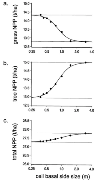
Compared to PAR absorption efficiency or wa-ter fluxes, NPP was the most sensitive variable to cell basal dimensions. Total grass NPP increased from 12.79 to 14.34 t ha− 1 (12.1% variation)
Fig. 8. Effects of cell basal dimensions on (a) grass; (b) tree and (c) total net primary productions simulated over one vegetation cycle (1991). Logarithmic scale is used for cell basal side size. Dots represent simulations, thick lines represent non linear regressions and thin lines are regression asymptots. All figures are at the same scale.
Fig. 7. Measured () (Gauthier, 1993) and simulated (o) total tree PAR absorption efficiency as a function of total tree LAI.
when cell basal side size decreased from 3 to 0.375 m, respectively (Fig. 8a). On the opposite, total tree NPP decreased from 15.00 to 12.97 t ha− 1 (13.5% variation) (Fig. 8b). Total NPP decreased little with decreasing cell basal dimensions (1.7% variation) (Fig. 8c). Thus changing cell basal di-mensions affected primarily the NPP distribution between the grass and tree components more than the overall production.
In the case of a cell size of 30 m, as whole site dimensions were 3 × 3 m, the system was
homoge-neous (i.e. one grass layer fully overlapped by one tree layer). When cell size decreases, one can expect model outputs to reach an asymptotic state as the model approaches a cell size of zero (i.e. a contin-uous description of space). We fitted a logistic curve through non linear regression (PROC NLIN, SAS Institute, 1990) to NPP values as a function of log (cell basal side size). Values of NPP obtained for the maximal cell size (30 m) were used as asymptotes for the logistic curves (i.e. top asymp-totes for total and tree NPP, basal asymptote for grass NPP). The nonlinear fit algorithm converged in all cases and gave the following estimates for asymptotes corresponding to a cell size decreasing towards zero: 14.33 t ha− 1 for grass NPP (cor-rected R2= 0. 99, F
3,5= 8097636, PB0.0001), 12.92 t ha− 1for trees (corrected R2= 0.99, F
3,5= 107726, PB0.0001) and 27.25 t ha− 1for the total system (corrected R2= 0.99, F
3,5= 93992, PB 0.0001). These values are closed to those simulated with a cell size of 0.375 × 0.375 m.
4.5. Spatial patterns of NPP affected by tree spatial
distribution
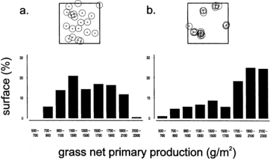
Fig. 9 presents the effects of tree spatial distribu-tion on grass NPP spatial heterogeneity. Overall
grass production with aggregated trees (17.66 t ha− 1) was 20% higher than with randomly dis-tributed trees (14.43 t ha− 1). When trees where randomly located (Fig. 9a) 93% of the site surface showed a grass NPP between 900 and 2100 g m− 2. When trees where aggregated (Fig. 9), high grass productions were more frequent: 67% of the sur-face showed a grass NPP above 1700 g m− 2. Thus both grass NPP spatial distribution and mean values at the site scale were strongly influenced by tree spatial structure.
5. Discussion
The RATP model and its ability to simulate the distribution of light regime, carbon acquisition and transpiration within plant foliage had already been tested by its authors (Sinoquet et al., 2000). The radiation absorption submodel ability to repro-duce grass radiation absorption had also been tested for a savanna grassland at Lamto (Le Roux et al., 1997). The production/water balance module of PEPSEE had been tested for savanna grasslands as well (Le Roux et al., 1996).
Our results showed that the model simulated quite accurately radiation, carbon and water
pro-Fig. 9. Differences in the simulated spatial distribution of grass net primary production over one vegetation cycle when trees are (a) randomly distributed or (b) highly aggregated. Plots above graphs show the sites used for simulations (14 × 14 m), with their tree spatial distributions. Tree number is 20 and all trees are identical (3.61 m high, canopy area of 4 m2).
cesses. These tests were done with integrative vari-ables (biomass, radiation absorption, soil water contents, NPP) involving the whole or at least a large part of the processes implemented in the model. In addition, simulations were done using different sites with varying tree spatial structure, making use of available field data for the Lamto savannas. Hence, TREEGRASS appears able to simulate the effects of vegetation structure on NPP and water balance of Lamto savannas, de-spite the absence of nutrients and rainfall inter-ception, and a simple tree architecture. However, these results also showed that the TREEGRASS model has some limits.
5.1. Plant radiation absorption
Tree PAR absorption efficiency was correctly simulated, except at the beginning of cycle, for low tree LAI, probably because stems and branches were not represented in the model. In the field, these organs are able to absorb some radiation when leaves are not fully expanded. Jackson et al. (1990) reported a radiation inter-ception efficiency of 0.25 for deciduous oaks with-out leaves. Stem material of numerous Texas savanna tree species showed a strong absorbance in a PAR spectral range, so that stem surfaces may have increased canopy PAR absorption effi-ciency by 10 – 40% when tree LAI was low (Asner et al., 1998). This could be implemented in the model if reliable and simple data were available on tree architecture in Lamto savannas. Anyway, it was not a major problem in our simulations as radiation absorbed by branches would not have been converted into dry matter, though stems could alter the spatial distribution of radiation absorption. When tree LAI is sufficiently high, this problem can be neglected.
A previous work showed that the radiation absorption submodel had a tendency to overesti-mate grass PAR absorption at the beginning of the vegetation cycle (data not shown but see Le Roux et al., 1997). This was potentially due to the fact that the grass stratum was assumed to be continuous throughout the year, although the grass layer is composed of tufts that do not fully cover the soil during the first two months of the
cycle. The importance of the grass fractional cover could be tested on a pure grass site, by explicitly taking into account grass spatial devel-opment at the beginning of the cycle.
5.2. Carbon processes
This overestimation of the grass PAR absorp-tion entailed an overestimaabsorp-tion of grass produc-tion at the beginning of each cycle (Fig. 4).
The simulated reduction of grass NPP under tree clump was slightly higher than that observed in the field, this could be due to the fact that the model did not treat nutrients, as higher nutrient availability is expected under tree cover (Mordelet et al., 1993). As already mentioned, we plan to add nutrient processes in TREEGRASS.
5.3. Water processes
The overestimation of the grass radiation ab-sorption could also be responsible for an underes-timation of soil evaporation at the beginning of the vegetation cycle. This effect could explain why TREEGRASS overestimated the soil water con-tent in layer 1 at the beginning of each cycle. Other reasons for this overestimation could be a possible different soil albedo after fire with the presence of ash during 1 to 3 weeks (Le Roux et al., 1994), and a change in the soil surface status at the end of the dry season that would have increased the runoff. These two possibilities were not computed, sensitivity analyses are needed to test these hypotheses.
The seasonal course of water content in soil layer 2 under a tree clump was not tested because of lack of data. For the same reason, the parti-tioning of evapotranspiration between evapora-tion, grass and tree transpiration rates could not be tested. It is clear that it would be interesting to test the model ability to simulate the evaporation rate according to the tree spatial distribution, and the relative importance of tree and grass transpi-ration rates. In particular, comparing the simu-lated tree transpiration with measured sap flow rates (e.g. Howard et al., 1997) is needed. Grass transpiration is more difficult to measure: using gas exchange chambers (Tournebize et al., 1996),
for instance, can alter the microclimate experi-enced by grasses.
Finally, it appeared that, despite of the absence of rainfall interception by the foliage, the model correctly simulated the grass behaviour in the absence of trees. A few data are available for rainfall interception by grass at Lamto and could be used to include this process in the model.
5.4. Importance of the size of grid cells
The smaller the cell size, the more accurate the representation of the tree crown shape, and the more accurate the simulation of competition for light. The ideal size would be the one under which there is no variation (in NPP for instance). The smallest cell size that a computer could handle for the tests was 0.375 × 0.375 m, and it seems that, from the non linear regression fit, it was very close to the ideal cell size. For larger sites, like those presented in Fig. 9, with sizes compatible with the scale of an ecosystem study, the cell size limit for computers became l × l m. This was applied to all test simulations as an acceptable compromise be-tween precision and computer requirements. This does not mean that plots used for simulations should be small. The maximum plot size depends mainly on the type of vegetation: the denser the vegetation, the higher the number of vegetation cells, and the longer the simulations.
5.5. Spatial heterogeneity of grass NPP and tree
spatial distribution
Due to their size, trees have first access to light. When trees were aggregated, there were larger open areas, i.e. more grass surface where there was no or little tree influence. These open areas showed a high grass NPP. On the opposite, a random distribution was associated with more isolated trees, and thus entailed stronger interac-tions between trees and grasses. These results emphasize the interest to study effects of the vegetation spatial structure on radiation, carbon, and water fluxes. Knowing when fine tree spatial structure needs to be considered for the function-ing of an ecosystem is one important purpose of TREEGRASS.
6. Conclusion
Tests described in this paper and using a 1 × 1 m resolution were conclusive:
1. Seasonal variations in biomass, necromass and soil water contents in layers 1 and 2 were satisfactorily simulated by the model in the case of a pure grass site.
2. Primary production values computed by the model were consistent with values reported in the literature.
3. The model correctly simulated the seasonal course of the soil water content in layer 1 under tree clump.
4. Tree PAR absorption efficiency was also cor-rectly simulated.
As already mentioned, the model described in this paper must be considered as a first version. In the near future, we plan to add mechanistic compu-tations for nitrogen processes, photosynthesis and a better tree architecture, in order to build a complete mechanistic model able to simulate daily savanna functioning. Breshears et al. (1997) found that, in New Mexico semiarid woodlands, two different tree species exploited soil water differ-ently. A similar conclusion was raised by Le Roux and Bariac (1998) at Lamto. Other studies showed that grass species composition can be different under tree cover or in open areas (e.g. Belsky et al., 1993; Scholes and Archer, 1997). Thus, it appears necessary to introduce more species in our simula-tions, in order to account for functional diversity. In the near future, TREEGRASS will be used to assess (1) the influence of tree spatial structure on total carbon and water fluxes at the site level (which is currently under progress); (2) the spatial and temporal distributions of production and water fluxes between individuals; (3) the effects of differ-ent tree types (e.g. deciduous versus evergreen, deep-rooted versus shallow rooted) on tree – grass interactions.
Acknowledgements
This work was supported by the European Ter-restrial Ecosystem Modelling Activity (ETEMA) and by the Programme National de Recherche en
Hydrologie (grant 99-PNRH 14, publication c189).
References
Abbadie, L., 1983. Aspects fonctionnels du cycle de l’azote dans la strate herbace´e de la savanne de Lamto. Ph.D. Thesis, University Paris, pp. 158.
Amadou, M., 1994. Analyse et mode´lisation de l’e´vapotran-spiration d’une culture de mil en re´gion sahe´lienne. Ph.D. Thesis, University Paris, pp. 106.
Asner, G.P., Wessman, C.A., Archer, S., 1998. Scale depen-dence of absorption of photosynthetically active radiation in terrestrial ecosystems. Ecol. Appl. 8, 1003 – 1021. Baruch, Z., Ludlow, M.M., Davis, R., 1985. Photosynthetic
responses of native and introduced C4 grasses from
Venezuelan savannas. Oecologia 67, 388 – 393.
Belsky, A.L, 1994. Influences of trees on savanna productiv-ity: tests of shade, nutrients, and tree – grass competition. Ecology 75 (4), 922 – 932.
Belsky, A.J., Mwonga, S.M., Amundson, R.G., Duxbury, J.M., Ali, A.R., 1993. Comparative effects of isolated trees on their undercanopy environments in high- and low-rainfall savannas. J. Appl. Ecol. 30, 143 – 155. Breshears, D.D., Myers, O.B., Johnson, S.R., Meyer, C.W.,
Martens, S.N., 1997. Differential use of spatially hetero-geneous soil moisture by two semiarld woody species:
Pinus edulis and Juniperus monospenna. J. Ecol. 85, 289 –
299.
Brouwer, R., 1983. Functional equilibrium: sense or non-sense? Neth. J. Agric. Sci. 31, 335 – 348.
Ciret, C., Polcher, J., Le Roux, X., 1999. An approach to simulate the phenology of savanna ecosystems in the LMD general circulation model. Glob. Biogeochem. Cy-cles 13, 603 – 622.
Coughenour, M.B., 1994. Savanna-Landscape and regional ecosystem model, documentation. Fort Collins, Colorado State University, pp. 47.
Cruz, P., 1997. Effect of shade on the growth and mineral nutrition of a C4 perennial grass under field conditions.
Plant Soil 188, 227 – 237.
De Jong, K., 1983. Research on the water balance in a savannah ecosystem. A Study for Two Soil Types at Lamto, Ivory Coast Internal Report, ENS, pp. 73. Dewar, R.C, Medlyri, B.E., McMurtrie, R.E., 1998. A
mech-anistic analysis of light and carbon use efficiencies. Plant Cell Env. 21, 573 – 588.
Durand, J.L., Lemaire, G., Gosse, G., Chartier, M., 1989. Analyse de la conversion de l’e´nergie solaire en matie`re se´che par un peuplement de (Medicago sati6a L.) soumis a` un de´ficit hydrique. Agronomie 9, 599 – 607.
Eagleson, P.S., Segarra, R.L, 1985. Water-limited equilibrium of savanna vegetation systems. Water Resour. Res. 21 (10), 1483 – 1493.
Gauthier, H. 1993. Echanges radiatifs et production primaire dans une savane humide d’Afrique de l’Ouest
(Lamto-Coˆte d’Ivoire). Master Thesis, CESR University Paul Sa-batier Toulouse, pp. 37.
Gignoux, L, Menaut, LC., Noble, L.R., Davies, I.D., 1996. A spatial model of savanna function and dynamics: model description and preliminary results. In: Prins, H.H.T., Brown, N. (Eds.), Dynamics of Tropical Communities, the 37th Symposium of the British Ecological Society. Blackwell, Oxford, pp. 361 – 383.
Howard, S.B., Ong, C.K., Black, C.R., Khan, A.A.H., 1997. Using sap flow gauges to quantify water uptake by tree roots from beneath the rooting zone in agroforestry sys-tems. Agrofor. Syst. 35, 15 – 29.
Isichei, A.O., Muoghalu, J.L, 1992. The effects of tree canopy cover on soil fertility in a Nigerian savanna. J. Trop. Ecol. 8, 329 – 338.
Jackson, L.E., Strauss, R.B., Firestone, M.K., Bartolome, J.W., 1990. Influence of tree canopies on grassland pro-ductivity and nitrogen dynamics in deciduous oak sa-vanna. Agric. Ecosyst. Environ. 32, 89 – 105.
Jarvis, P.G., 1976. The interpretation of the variations in leaf water potential and stomatal conductance found in canopies in the field. Phil. Trans. R Soc. Lond. B 273, 593 – 610.
Jeltsch, R, Milton, S.L, Dean, W.J.R., Van Rooyen, N., 1996. Tree spacing and coexistence in semi-arid savannas. J. Ecol. 84, 583 – 595.
Joffre, R., Rambal, S., 1988. Soil water improvement by trees in the rangelands of southern Spain. Acta Oecol. (Oecol. Plant.) 9 (4), 405 – 422.
Knoop, W.T., Walker, B.H., 1985. Interactions of woody and herbaceous vegetation in a southern african savanna. J. Ecol. 73, 235 – 253.
Korzukhin, M.D., Ter-Mikaelian, M.T., 1996. An individual tree-based model of competition for light. Ecol. Model. 79, 221 – 229.
Landsberg, J.J., Waring, R.H., 1997. A generalised model of forest productivity using simplified concepts of radiation-use efficiency, carbon balance and partitioning. For. Ecol. Manag. 95, 209 – 228.
Le Provost, E., 1993. Structure et fonctionnement de la strate herbace´e d’une savane humide (Lamto, Coˆte d’Ivoire). Master Thesis, University Paris, pp. 38.
Le Roux, X. 1995. Etude et mode´lisation des e´changes d’eau et d’e´nergie sol-ve´ge´tation atmosphe`re dans une savane humide (Lamto, Coˆte d’Ivoire). Ph.D. Thesis, University Paris, pp. 203.
Le Roux, X., Bariac, T., Mariotti, A., 1995. Spatial partition-ing of the soil water resource between grass and shrub components in a West African humid savanna. Oecologia 104, 147 – 155.
Le Roux, X., Bariac, T., 1998. Seasonal variation in soil, grass and shrub water status in a West African humid savanna. Oecologia 113, 456 – 466.
Le Roux, X., Polcher, J., Menaut, LC., Monteny, B.A., 1994. Radiation exchanges above West African moist savannas: seasonal patterns and comparison with a GCM simula-tion. J. Geophys. Res. 99 (112), 25 857 – 25 868.
Le Roux, X., Tuzet, A., Zurfluh, O., Gignoux, L., Perrier, A., Monteny, B.A., 1996. Mode´lisation des interactions sur-face/atmosphe`re en zone de savane humide. In: Hoepffner, M., Lebel, T., Monteny, B. (Eds.), Interactions Surface Continentale/Atmosphe`re: l’expe´rience HAPEX – SAHEL. ORSTOM Editions, pp. 303 – 317.
Le Roux, X., Gauthier, H., Be´gue´, A., Sinoquet, H., 1997. Radiation absorption and use by humid savanna grassland: assessment using remote sensing and modelling. Agric. For. Meteorol. 85, 117 – 132.
Le Roux, X., Grand, S., Dreyer, E., Daudet, F.A., 1999. Parameterisation and testing of a biochemically based pho-tosynthesis model for walnut (Juglans regia) trees and seedlings. Tree Physiol. 19, 481 – 492.
Littleboy, M. and McKeon, G.M., 1997, Evaluating the risks of pasture and land degradation in native pastures in Queensland — Appendix 2 — Subroutine GRASP: grass production model. Indooroopilly: Rural Industries Re-search and Devlopment Corporation.
Medina, E., 1982. Physiological ecology of neotropical sa-vanna plants. In: Huntly, B.J., Walker, B.H. (Eds.), Ecol-ogy of Tropical Savannas, pp. 308 – 335.
Medina, E., Francisco, M., 1994. Photosynthesis and water relations of savanna tree species differing in leaf phenology. Tree Physiol. 14, 1367 – 1381.
Menaut, J.C., 1974. Chutes de feuilles et apport au sol de litie`re par les ligneux dans une savane pre´forestie`re de Coˆte d’Ivoire. Bull. d’Ecol. 5, 27 – 39.
Menaut, J.C., Ce´sar, J., 1979. Structure and primary produc-tivity of Larrito savannas, Ivory Coast. Ecology 60, 1197 – 1210.
Monteith, J.L, 1972. Solar radiation and productivity in tropi-cal ecosystems. J. Appl.Ecol. 2, 747 – 766.
Monteith, J.L., 1977. Climate and the efficiency of crop pro-duction in Britain. Phil. Trans. R Soc. Lond. 281, 274 – 277. Moon, P., Spencer, D.E., 1942. Illumination from a
non-uni-form sky. Trans. Illum. Eng. Soc. 37, 707 – 712.
Mordelet, P, 1993. Influence des arbres sur la strate herbace´e d’une savane humide (Lamto, Coˆte d’Ivoire). PhD. Thesis, University Paris 6, pp. 150.
Mordelet, P., Menaut, L.C., 1995. Influence of trees on above-ground production dynamics in a humid savanna. J. Veg. Sci. 6, 223 – 228.
Mordelet, P., Abbadie, L., Menaut, J.C., 1993. Effects of tree clumps on soil characteristics in a humid savanna of West Africa (Lamto Coˆte d’Ivoire). Plant Soil 153, 103 – 111. Ozisik, N.M., 1981. Radiative Transfer. Wiley, New York, p.
575.
Pacala, S.W., Deutschman, D.H., 1995. Details that matter: the spatial distribution of individual trees maintains forest ecosystem function. Oikos 74, 357 – 365.
Parton, W.J., 1996. The CENTURY model. In: Powlson, D.S., Smith, P., Smith, J.U. (Eds.), Evaluation of soil organic matter models. Springer-Verlag, Berlin, pp. 283 – 294.
Rhoades, C.C., 1997. Single-tree influences on soil properties in agroforestry: lessons from natural forest savanna ecosys-tems. Agrofor. Syst. 35, 71 – 94.
SAS Institute, 1990. SAS/STAT user’s guide, SAS institute, Cary.
Scholes, R.J., Archer, S.R., 1997. Tree – grass interactions in savannas. Annu. Rev. Ecol. Syst. 28, 517 – 544.
Scholes, R.J., Hall, D.O., 1996. The carbon budget of tropical savannas, woodlands and grasslands. In: Hall, D.O., Breymeyer, A.I., Mellilo, J.M., Agren, G.I. (Eds.), Global Change: Effects on Coniferous Forests and Grasslands, SCOPE. Wiley, New York, pp. 69 – 100.
Schulze, E.D., 1994. Relationships among stomatal conduc-tance, carbon assimilation rate, and plant nitrogen nutri-tion: a global ecology scaling exercise. Annu. Rev. Ecol. Syst. 25, 629 – 660.
Simoes, M., Baruch, Z., 1991. Responses to simulated her-bivory and water stress in two tropical C4grasses.
Oecolo-gia 88, 173 – 180.
Sinoquet, H., Bonhomme, R., 1992. Modeling radiative trans-fer in mixed and row intercropping systems. Agric. For. Meteorol. 62, 219 – 240.
Sinoquet, H., Le Roux, X., Ame´glio, T., Daudet, F.A., 2000. Mode´lisation de la distribution spatiale du microclimat lumineux, de la transpiration et de la photosynthe`se appli-cation a` un arbre isole´. In: Maillard, P., Bonhomme, R. (Eds.), Fonctionnement des Peuplements Ve´ge´taux sous Contraintes Environnementales. INRA Editions, Se´rie Les Colloques, Paris, pp. 185 – 199.
Solbrig, O., Menaut, J.C., Mentis, M., Shugart, H.H., Stott, P., Wigston, D., 1990. Savanna modelling for global change. Biol. Int. 24, 3 – 45.
Stuart-Hill, G.C., Tainton, N.M., 1989. The competitive inter-action between Acacia karroo and the herbaceous layer and how it is influenced by defoliation. J. Appl. Ecol. 26, 285 – 298.
Sueur, J., 1995. Comparaison des e´changes gazeux foliaires de diffe´rents ge´notypes d’une gramine´e de savane
(Hyparrhe-nia diplandra). Master Thesis, ENS Lyon.
Tournebize, R., Sinoquet, H., Bussie`re, F., 1996. Modelling evapotranspiration partitioning in a shrub/grass alley crop. Agric. For. Meterol 81, 255 – 272.
Ullman, I., 1985. Diurnal courses of transpiration and stomatal conductance of sahelian and saharian acaias in the dry season. Flora 176, 383 – 409.
Walker, B.H., Ludwig, D., Holling, C.S., Peterman, R.M., 1981. Stability of semi-arid savanna grazing systems. J. Ecol. 69, 473 – 498.
Weishampel, J.F., Urban, D.L., 1996. Coupling a spatially-ex-plicit forest gap model with a 3-D solar routine to simulate latitudinal effects. Ecol. Modelling 86, 101.
Weltzin, J.F., Coughenour, M.B., 1990. Savanna tree influence on understory vegetation and soil nutrients in northwestern Kenya. J. Veg. Sci. 1, 325 – 334.