1
Better Multivalent Battery Materials through Diffusion High-throughput
Computations
by Ziqin Rong
Submitted to the Department of Materials Science and Engineering and the Department of Electrical Engineering & Computer Science in Partial Fulfillment of the Requirements for Degrees of
Master of Science in Materials Science and Engineering and Master of Science in Electrical Engineering & Computer Science
at the
Massachusetts Institute of Technology June 2016
© 2016 Massachusetts Institute of Technology. All Rights Reserved
Signature of Author...……….. Department of Materials Science and Engineering Department of Electrical Engineering & Computer Science May 19, 2015 Certified by … ………
Gerbrand Ceder Professor of Materials Science and Enginnering Thesis Supervisor ………
Patrick Winston Professor of Artificial Intelligence and Computer Science Thesis Reader Accepted by ………. Donald Sadoway Professor of Materials Science and Engineering Chair, Materials Science & Engineering Committee on Graduate Students .……… Leslie Kolodziejski Professor of Electrical Engineering & Computer Science Chair, Electrical Engineering & Computer Science Committee on Graduate Students
2
Better Multivalent Battery Materials through
Diffusion High-throughput Computations
by Ziqin Rong
Submitted to the Department of Mechanical Engineering and the Department of Electrical Engineering and Computer Science in Partial Fulfillment of the Requirement for Degrees of
Master of Science in Materials Science and Engineering and Master of Science in Electrical Engineering and Computer Science
Abstract:
Accelerating the discovery of advanced materials is essential for human beings. However, the traditional trial-and-error way of developing materials is often very empirical and time- consuming. In 2011, the launch of Materials Genome Initiative marked a large-scale collaboration between computer scientists and materials scientists to deploy proven computational methods to predict, screen, and optimize materials at an unparalleled scale and rate. This thesis is based on this idea. Finding a suitable cathode material for Mg batteries has been one of the key challenges to the next-generation multi-valent battery technology. In this thesis, a high-throughput computation system is proposed to solve such problem. I tested the high-throughput structures applying traditional NEB calculations schemes and find out it is very different to scale traditional NEB method to a high-throughput application. Then I proposed a new scheme for estimating migration minimum- energy path (MEP) geometry and energetics (PathFinder and ApproxNEB). By testing our methodology against standard NEB calculations and literature values, we find that the PathFinder algorithm can reliably predict the geometry of cation migration MEP within 0.2 Å at negligible computational cost. Furthermore, we
3
find that the ApproxNEB calculation scheme yields activation barriers for migration within an error bound of 20 meV while using significantly fewer computational resources than NEB. We envision that our methods can be used to accelerate NEB calculations, as well as to provide a robust estimation criterion for migration barriers in ionic materials for high-throughput computational screening of materials. Based upon these two newly developed methods, coupled with EndPointFinder, I developed two functional high-throughput applications (ApproxNEB for estimating migration barriers and PathFinder for calculating migration geometric paths), and have already put PathFinder high-throughput system into production and calculate around 2000 structures.
4
Acknowledgements
I would like to acknowledge and thank my advisor, Prof. Gerbrand Ceder. He offered me with the opportunity and support for a fantastic project and gave me. And I have learned so much from discussing science with him.
I also want to give my deep appreciation for Prof. Patrick Winston. His insight into algorithm-related work stimulates me a lot through the way of this project.
I want to thank my collaborator Daniil Kitchaev. His work in PathFinder algorithm is the foundation of the ApproxNEB method I developed. I would also like to thank my lab mates Wenxuan Huang and Piero Canepa, who have leveraged their individual expertise to help develop the theory part of this thesis.
Anubhav Jain from LBNL has been a constant source of generous help in implementing the high-throughput ApproxNEB system with Fireworks system, to which I own great gratitude.
Last but not least, I want thank my parents and my girlfriend Xinyi, for their support, love and everything.
5
Contents
Acknowledgements ... 4
Chapter 1 Introduction ... 6
1.1 Problem and Motivation ... 6
1.2 Nudged Elastic Band Methodology ... 11
1.3 High-throughput Computations ... 14
Chapter 2 High-throughput NEB system ... 15
2.1 Framework ... 16
2.2 Obstacles ... 19
Chapter 3 PathFinder Algorithm ... 20
3.1 Methods ... 21
3.2 Error Metric Definition ... 24
3.3 PathFinder v.s. Linear Interpolation on Error Metric ... 25
3.4 PathFinder v.s. Linear Interpolation on Computational Resource Cost ... 27
3.5 PathFinder v.s. Linear Interpolation on CaMoO3 example ... 28
Chapter 4 ApproxNEB Method ... 29
4.1 Methods ... 30
4.2 ApproxNEB v.s. NEB on Barrier Estimation ... 32
4.3 ApproxNEB v.s. NEB on Computational Resource Cost ... 33
4.3 ApproxNEB Implementation ... 35
Chapter 5 High-throughput ApproxNEB Framework ... 37
5.1 Error Handling ... 37
5.2 EndPointFinder ... 38
5.3 Framework ... 42
Chapter 6 Conclusions and Contributions ... 44
6
Chapter 1
Introduction
1.1 Problem and Motivation
The energy density requirements of next-generation mobile electronics, electrified vehicles, and renewable energy storage are rapidly outpacing the limit of what is theoretically possible with traditional intercalation-based Li-ion batteries, the current and longstanding industry workhorse.1,2 While many new approaches can potentially offer
benefits in terms of cost, safety, and specific energy,1,3 there are very few options for high
energy density (e.g. by volume) which is a critical performance metric in many applications. One promising strategy is to go to a multi-valent (MV) chemistry by pairing a MV metal anode (such as Mg, for instance) with a cathode that can reversibly store those MV ions.4 Such a cell may be able to achieve energy density well over 1000 Wh/L due to
the high volumetric capacity of metal anodes (3830 Ah/L and 8040 Ah/L for Mg and Al, respectively, compared to ~700 Ah/L for Li in C) and the high capacity that may be achieved with MV insertion cathodes.2 But the challenges of realizing such a multi-valent
battery chemistry are many and complex in nature, which highlight the importance of acquiring fundamental knowledge early on in order to identify the research directions that are most likely to bear fruit. The challenges for MV anodes and electrolytes have been well documented,5 and in this thesis we focus on understanding and charting the
challenge posed by creating cathode host structures with sufficient MV cation mobility required for reversible intercalation at reasonable rates. Indeed, the expectation is that the higher charge of MV cations will polarize a host’s environment, thereby reducing mobility and rate capability of MV chemistries. This is a very critical issue because with low
7
mobilities (we also use diffusivities in this proposal for the same meaning), even though we are able to identify a MV cathode material with high energy density, we will still be unable to charge or discharge the battery because the moving rates of cations in cathode are so low. While for Li+ intercalation both extensive experimental6-8 and theoretical9-14 Li
mobility data are readily available, the lack of reliable electrochemical MV test vehicles5,15
and limited exploration of MV chemistries have made it difficult to understand what controls MV ion mobilities.
Although the concept of a rechargeable magnesium battery was proposed as early as 1990,30 the first working demonstration of a prototype Mg full cell battery was achieved
in 2000 by Aurbach et al.31 using a magnesium metal anode, an electrolyte based on a
solution of Mg organo-halo-aluminate salts in tetrahydrofuran (THF), and a Chevrel MgxMo6S8 cathode (0 < x ≤ 2). With these innovations at the electrolyte and cathode, they
were able to achieve ~1.4 V vs. Mg metal and ~80 mAh/g (128.8 mAh/g theoretical capacity), with good kinetics and cycle life (> 2000 cycles). On the process of discovering the Chevrel phase as a Mg intercalation host, we remarked that it was the result of “a lot of unsuccessful experiments of Mg ions insertion into well-known host for Li+ ions insertion, as well as from the thorough literature analysis concerning the possibility of divalent ions intercalation into inorganic materials.”32 Of note, batteries based on Chevrel compounds
were proposed and demonstrated to function for Li-ion as early as 1985.33
Unlike today’s commercialized Li-ion cathode materials, which are almost entirely structures with close-packed oxygen anion sub-lattices (e.g., layered, spinel, olivine), the Chevrel phase has a unique “cluster” structure shown below in Figure 1. The Chevrel
8
structure is comprised of Mo6T8 (T = S, Se, Te) blocks (gray cubes in Figure 1a), with 6 Mo
forming an octahedron on the faces and 8 T anions occupying the corners. 34-35 The Mo 6S8
blocks are arranged such that they are separated by three types of “cavities” as illustrated in Figure 1b, and the intercalation sites are contained within cavities of type 1 and 2. The site position within each cavity varies with cation species, 37 but for small ions (such as Li+,
Mg2+, or Cu1+/2+ compared to Pb2+ or Sn2+) there are multiple intercalation sites available
within each cavity as shown in the inset of Figure 1b, with a ring of “inner sites” within cavity 1 and two “outer sites” in cavity 2. Considering the topology of Mo6S8 blocks, there
are twelve possible sites (6 inner and 6 outer) between each block where the intercalating ion can reside as seen in Figure 1.38 The Mo octahedral clusters exhibit metallic bonding
and are each capable of accommodating a total of 4 electrons.49 Accordingly, two Mg2+
9
Fig. 1 Chevrel Crystal Structure36
accommodated preferentially in the inner sites and the second in the outer sites. This is reflected in the voltage curve, voltage plateaus that occur at ∼ 1.4 V and ∼ 1.1 V, respectively, in Fig 2.40
10
Fig. 2 oltage-capacity curve of Mg insertion into Mo6S8
The un-intercalated Chevrel Mo6S8 structure is thermodynamically unstable, but can be
obtained metastably by first synthesizing CuMo6S8 commonly through element solid-state
reaction (or alternatively through lower temperature precipitation methods),41 followed by
acid leaching Cu from the synthesized phase.42–44
Several different monovalent, divalent, and recently trivalent cations45 have shown
mobility within the Chevrel structure.46 For example, the electrochemically extracted
diffusivities for Co2+, Ni2+, Fe2+, Cd2+, Zn2+, and Mn2+ are quite high in Mo
6S8, ∼10−9
cm2/s,47
compared to ∼10−11−10−13 cm2/s for Mg2+.48 As mentioned earlier, different cations
occupy different sites within Cavity 1 and Cavity 2, which contributes to the complex mobility behavior observed across varying cation species. 46 For example, poor mobility is
observed for large cations such as Pb2+, Sn2+, and Ag+ compared to smaller cations such as
Ni2+, Zn2+, and Li+ in the ternary structure (e.g. MMo
6T8), but in mixed cation systems (e.g.
11
insertion-displacement reactions.49-50 Notably, the presence of Cu in the host structure has
a beneficial effect on the Mg2+ intercalation kinetics.50-51
Mg intercalation in Chevrel structures represents state-of-the-art performance in MV batteries, displaying excellent reversibility and intercalation kinetics. As a matter of fact, it has been the only workable cathode materials for Mg batteries till now, though great effort has been spent to look into similar open structures to Chevrel phases.
1.2 Nudged Elastic Band Methodology
The nudged elastic band (NEB) method is an efficient method for finding the minimum energy path (MEP) between a given initial and final state of a transition.16–18 It
has become widely used for estimating transition rates within the harmonic transition state theory (hTST) approximation. The method has been used both in conjunction with electronic structure calculations, in particular plane wave based density-functional theory (DFT) calculations 19–22, and in combination with empirical potentials. 23–25 Studies of very
large systems, including over a million atoms in the calculation, have been conducted. 26
The MEP is found by constructing a set of images (replicas) of the system, typically on the order of 4–20, between the initial and final state. A spring interaction between adjacent images is added to ensure continuity of the path, thus mimicking an elastic band. An optimization of the band, involving the minimization of the force acting on the images, brings the band to the MEP. An essential feature of the method, which distinguishes it from other elastic band methods, 27-29 is a force projection which ensures that the spring forces
12
that the true force does not affect the distribution of images along the MEP. It is necessary to estimate the tangent to the path at each image and every iteration during the minimization, in order to decompose the true force and the spring force into components parallel and perpendicular to the path. Only the perpendicular component of the true force is included, and only the parallel component of the spring force. This force projection is referred to as ‘‘nudging.’’ The spring forces then only control the spacing of the images along the band. The spring forces then only control the spacing of the images along the band. When this projection scheme is not used, the spring forces tend to prevent the band from following a curved MEP because of ‘‘corner-cutting’’, and the true force along the path causes the images to slide away from the high energy regions towards the minima, thereby reducing the density of images where they are most needed (the ‘‘sliding-down’’ problem). In the NEB method, there is no such competition between the true forces and the spring forces; the strength of the spring forces can be varied by several orders of magnitude without effecting the equilibrium position of the band.
The MEP can be used to estimate the activation energy barrier for transitions between the initial and final states. Like the Fig. 1 below is a demonstration of NEB calculations, which characterizes the system energy when cations (Li+, Mg2+, Zn2+, Ca2+,
Al3+) migrate from one stable position to the nearest stable position in TiS
2 layer host
structure. From the MEP, we can obtain the activation energy, which is the peak energy point on the curve (saddle point).
An upper bound for the MV migration barrier Em can be established from
13
active particle size suggests a minimum diffusivity D ~ 10–12 cm2s–1 given the diffusion
length scales as . Using a random walk for diffusion sets a maximum Em ~ 525 meV
that can be tolerated, assuming D ≈ ν · a2 · exp(–E
m/kT) with atomic jump frequency ν ≈
1012 s–1 and atomic jump distance a ≈ 3 Å, the length of a typical lattice parameter. For
every order of magnitude particle size reduction this tolerance increases by ~ 125 meV. Hence, 100 nm crystallites could be charged and discharged in 2 hours when barriers are less than ~ 650 meV. Note that reasonable ion diffusion is a required
Fig. 3 NEB calculation example, in TiS2 layer host structure
condition for cathode materials, but it is by no means sufficient as other phenomena, either in the cathode (e.g. phase transformations, conductivity) or in the cell, can be rate
Dt 0 10 20 30 40 50 60 70 80 90 100 Path Length [%] 0 100 200 300 400 500 600 700 800 900 1000 1100 1200 E [meV] Li (3.42 Å) Mg (3.42Å) Zn (3.42 Å) Ca (3.42 Å) Al (4.12 Å)
14
limiting. Nonetheless, solid-state diffusion is widely seen as the most challenging design problem for MV-cathode materials.
Thus if the NEB calculations show the migration barrier of Mg in certain structure is below the 525meV threshold, then it means that the host structure might be a potential cathode materials for Mg batteries.
1.3 High-throughput Computations
Materials discovery today involves significant trial-and-error. It can require decades of research to identify a suitable material for a technological application, and longer still to optimize that material for commercialization. A principal reason for this long discovery process is that materials design is a complex, multi-dimensional optimization problem, and the data needed to make informed choices about which materials to focus on and what experiments to perform usually does not exist.
What is needed is a scalable approach that leverages the talent and efforts of the entire materials community. The Materials Genome Initiative, launched in 2011 in the United States, is a large-scale collaboration between materials scientists (both experimentalists and theorists) and computer scientists to deploy proven computational methodologies to predict, screen, and optimize materials at an unparalleled scale and rate. Many research groups have already employed this high-throughput computational approach to screen up to tens of thousands of compounds for potential new technological materials. Examples include solar water splitters, 52-53 solar photovoltaics, 54 topological
15
insulators, 55 scintillators, 56-57 CO2 capture materials, 58 piezoelectrics, 59 and
thermoelectrics, 60-61 with each study suggesting several new promising compounds for
experimental follow-up. In the fields of catalysis, 62 hydrogen storage materials, 63-64 and
Li-ion batteries, 65-69 experimental “hits” from high-throughput computations have already
been reported.
Applying similar ideas from the Materials Genome Initiative project, if we can find whether one structure is good for being a Mg battery cathode materials by doing a NEB calculations, in principle if we build up a system where we can calculate NEBs over thousands of different materials, then we can pick the good one from the high-throughput calculation results. And that is the idea behind this thesis.
Chapter 2 High-throughput NEB system
NEB calculation is 3-step calculation:
Step 1. Execute DFT calculation of the starting point and ending point of the diffusion path. After choosing the host structure and the diffusing cation, a super cell structure is constructed for DFT calculations, with the moving cation in the starting and ending position.
Step 2. Extract the structure information from previous starting and ending point DFT calculations, a diffusing path of the cation is interpolated between two end point structures. Because I’m using a guessing algorithm33 for the diffusion path, by the
16
requirement of the algorithm, an extra DFT calculation is necessary for finding an optimal path to start the NEB DFT calculation.
Step 3. Starting from the interpolated guessing path, execute NEB relaxation DFT calculations.
Thus, the first system I tried is to put this normal manual calculation into high-throughput automatic system.
2.1 Framework
The automatic job tree structure is shown in Fig. 4. It’s roughly the same structure of the 3 steps plus database extraction and insertion, except from the detour job structures that I added into the DFT calculations of Step 1 and Step 3.
17
Fig. 4, Job structure tree for NEB calculations
The detours are designed as an error handler system. The design is to stop the calculations at certain frequency (e.g. every 10 hours), and have a script job to check the status of the previous DFT job. There are three possible different results for the check:
18
• There is an error found from the output of the previous job. Then corresponding corrections are made and a new job with such corrections is restarted from the initial state of previous job.
• There is no error found, but the previous job is not completed. Then a new job is created from the ending status of previous job.
• There is no error found and the previous job is completed. Then the detour structures are finished and the system returns back to the main tree for executing the next step.
To automate the dependencies of each job inside the job tree, I’m using a set codes called Fireworks, designed and implemented by my collaborator Anubhav Jain.70 It utilizes a workflow model:
• A FireTask is an atomic computing job. It can call a single shell script or execute a single Python function (either within FireWorks, or in an external package, like VASP for the DFT calculations).
• A FireWork contains the JSON spec that includes all the information needed to bootstrap the job. For example, the spec contains an array of FireTasks to execute in sequence. The spec also includes any input parameters to pass to the FireTasks.
• A Workflow is a set of FireWorks with dependencies between them.
Between FireWorks, a FWAction can be returned to store data or modify the Workflow depending on the output
19 In summary:
𝑊𝑜𝑟𝑘𝑓𝑙𝑜𝑤 = 𝐴 𝑠𝑒𝑡 𝑜𝑓 𝐹𝑖𝑟𝑒𝑊𝑜𝑟𝑘𝑠 + 𝑑𝑒𝑝𝑒𝑛𝑑𝑒𝑛𝑐𝑖𝑒𝑠 𝑏𝑒𝑡𝑤𝑒𝑒𝑛 𝐹𝑖𝑟𝑒𝑊𝑜𝑟𝑘𝑠 𝐹𝑖𝑟𝑒𝑊𝑜𝑟𝑘 = 𝐴 𝑠𝑒𝑡 𝑜𝑓 𝐹𝑖𝑟𝑒𝑇𝑎𝑠𝑘𝑠 + 𝑙𝑖𝑛𝑒𝑎𝑟 𝑠𝑒𝑞𝑢𝑒𝑛𝑐𝑒 𝑜𝑓 𝐹𝑖𝑟𝑒𝑊𝑜𝑟𝑘𝑠 + 𝑠𝑝𝑒𝑐
𝐹𝑖𝑟𝑒𝑇𝑎𝑠𝑘 = 𝐴 𝑠𝑐𝑟𝑖𝑝𝑡 𝑜𝑟 𝑎 𝑐𝑎𝑙𝑙 𝑓𝑜𝑟 𝑒𝑥𝑡𝑒𝑟𝑛𝑎𝑙 𝑝𝑟𝑜𝑔𝑟𝑎𝑚
Each of the green blocks in Fig. 4 is a FireWork. And the tree depicts the dependencies among them. Detours and data passing between FireWorks are created or done by returning FWAction.
2.2 Obstacles
After implementing this high-throughput machine with some effort, the system is capable of reproducing the manual results (Fig. 5).
20
Fig. 5 High-throughput NEB results comparing with manual NEBs, Li migration in Mn2O4 spinel structure
However, when I put more structures into the system, the job failure rates turn out to be really high (>60%) and most of the job errors can’t be easily dealt with. The other problem I am facing is high-throughput NEB consumes a great amount of computation resources (CPU hours), which limit the method to be applied to a wider range of structures database.
Chapter 3 PathFinder Algorithm
The standard workflow for the NEB calculation consists of 3 main steps: • Step 1. Relax the initial and final state structures.
• Step 2. Linearly interpolate a number of images between initial and final states. • Step 3. Apply the NEB algorithm to compute the MEP.
We find that the linear interpolation in Step 2 is the primary source of inefficiency and instability in the calculation procedure. This is especially true if the final MEP displays substantial curvature from the initial linear interpolation. Furthermore, during the preparation of the NEB calculation in some systems, the linear interpolation can place atoms (of one image) at unreasonably close distances to one another, causing instability
21
during the NEB relaxation (see for example, the CaMoO3 structure in the section 3.7). Here
we present a new method to initialize the NEB interpolation close to the final relaxed band that we call PathFinder Algorithm. In the following sections we discuss the idea behind the PathFinder algorithm and give details about its implementation. We also test the PathFinder algorithm on a set of six materials, demonstrating its predictive capabilities and the computational runtime reduction it brings.
3.1 Methods
In the NEB algorithm, each image along the band is relaxed by two forces – the true force from the potential and the spring force (from the virtual springs) connecting adjacent images. Note that both forces are decomposed into components perpendicular and parallel to the path, and only the perpendicular component of the true force and parallel component of spring force are relaxed in the NEB procedure. The force projection is referred to as ‘nudging’ and leads the chain of images to the MEP. To predict the MEP with fewer computational resources, we would like to imitate this relaxation process starting from a static potential. As the spring forces are very easy to simulate, the difficulty lies in finding a potential field that is able to reproduce the true force from first-principle calculations.
The key idea behind PathFinder is that when an atom migrates inside a host structure, it moves to avoid atoms or bonds, as atomic charge density overlap with other species would correspond to reactions, or at least large changes in energy. Consequently,
non-22
reactive migration paths should avoid concentrations of electronic charge density. Thus, we propose using the electronic charge density obtained from DFT as the potential landscape within which to estimate the migration MEP. In general, this potential will push migrating atoms to regions of diminishing charge density, corresponding to areas void of atoms or bonds, matching the intuition regarding the migration path geometry.
Based on this construction, the migrating images relax according to the sum of two forces: 𝐹 = 𝐹!+ 𝐹! = ∇ 𝑐ℎ𝑎𝑟𝑔𝑒 𝑑𝑒𝑛𝑠𝑖𝑡𝑦 + 𝑘!"∙ 𝑟!!!− 𝑟! (1)
where 𝐹! is the force coming from the charge density ‘potential’, 𝐹! is the spring force, 𝑟! is the position of image 𝑛 in real space and 𝑘!" is the spring force constant for the
pathfinder, where all quantities are given in non-dimensional form. The non-dimensional spring constant 𝑘!" = 0.17 is a constant fit to best reproduce the paths from a full VASP
NEB calculation with a default NEB spring constant of 5.0 eV/Å2. The relaxation algorithm
we use for the migration path is the zero temperature string method (ZTS) described by Vanden-Eijnden et al.71-72 We choose the string method specifically because it
demonstrates superior performance to NEB when a large number of images can be used. 33
Finally, the positions of all non-migrating atoms can be interpolated linearly for the intermediate images, as their positions are nearly static and thus reasonably represented by the linear path.
23
1. The initial state structure (structure of the atom-vacancy pair pre migration jump) 2. The final state structure (structure of the atom-vacancy pair post migration jump) 3. The charge density of the host structure
For illustration, Fig. 1 depicts the three inputs to compute Li diffusion paths in LiFePO4
along the b axis, 73 where in the initial and final states Li-ions sit in the stable sites. The
PathFinder algorithm relaxes intermediate Li images along the migration path to positions on the MEP. To initialize the PathFinder algorithm we compute the charge density of the host structure using a static calculation with Γ−point sampling of reciprocal space, as we have found that the paths thus obtained are sufficiently converged for all test cases. The output of the PathFinder algorithm are the positions of the intermediate images which can then be used to initialize a NEB calculation. As the computational cost of the PathFinder itself is negligible compared to the full NEB calculation, we find that it is effective to use a large number of interpolated images in the PathFinder to ensure optimal convergence of the string method, and then pick a small set of evenly spaced images from the estimated MEP to initiate the full NEB calculation.
The complete code set and example for using the algorithm can be found at the referenced github code repo.74The code implementation depends on the Python Materials Genomics (pymatgen) Library. 75
24
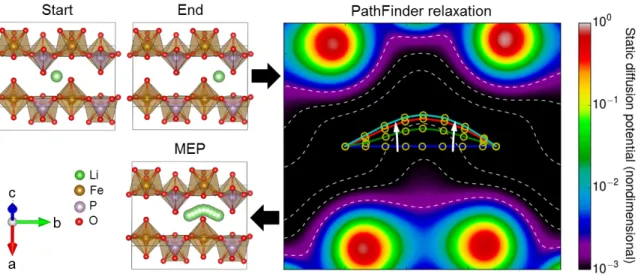
Figure 6. Illustration of the PathFinder Algorithm for an example of Li migration in LiFePO4
(Li in green, O in red, Fe in brown, and P in purple) projected onto the plane-of-best-fit for the MEP. The upper left panel shows the initial and final states of the Li migration jump, which serve as the inputs to the PathFinder algorithm. The right panel depicts the path relaxation in the PathFinder algorithm, where the path is relaxed through the virtual potential derived from the DFT electronic charge density and the spring force, where the potential is shown color-coded by magnitude with equipotential contours depicted by dashed lines, and with white arrows indicating the direction of relaxation. Finally, the lower left panel depicts the final relaxed Li MEP path produced by the PathFinder algorithm, which is in close agreement to the MEP obtained from a full NEB calculation (see Fig. 7b).
3.2 Error Metric Definition
To assess the capabilities of PathFinder and ApproxNEB we study cation migration in a set of materials that are of practical interest in the field of batteries. As we expect the PathFinder and ApproxNEB methods to yield improved performance relative to standard
25
NEB in cases where the migration paths deviate from straight-line paths, we report the curvature of the MEP as obtained by NEB calculations.
• Li in spinel LiTiS2 (linear MEP); 76-77
• Zn in spinel ZnMn2O4 (linear MEP); 78-79
• Zn in post-spinel ZnMn2O4 (linear MEP); 80
• Li in olivine LiFePO4 (curved MEP); 81-85
• Mg in δ-MgV2O5 (curved MEP); 86-69
• Ca in layered CaMoO3 (curved MEP). 90
3.3 PathFinder v.s. Linear Interpolation on Error Metric
The geometry error for the cation migration path for each benchmark material is given in Fig. 7. Specifically, for each material, we compare the error of the PathFinder path and the standard linear interpolation, with respect to the NEB-converged MEP, in order to understand which interpolation scheme can serve as a superior initialization. Note that while in the NEB calculations of the benchmark materials, seven images are used to interpolate the migration path, in the PathFinder Algorithm, we use 21 images to ensure good performance of the string method. Nonetheless, for consistency, in Fig. 7b, we use seven equally spaced images for visualization.
26
Figure 7. (a) Geometric error in the MEP initialization based on the PathFinder algorithm and linear interpolation across benchmark materials, illustrating the consistent performance of the PathFinder algorithm across both linear and curved MEP geometries. (b) A comparison of the migration path of Li in LiFePO4 and Mg in MgV2O5 obtained the PathFinder algorithm (black)
and the converged true MEP (green).
As is clear from Fig. 7a, if the fully relaxed NEB path possesses a large degree of curvature, the PathFinder algorithm systematically provides a better initialization than traditional linear interpolation. The migration path derived from the PathFinder algorithm falls within 0.2 Å of the NEB-derived MEP in all test structures, which is both a very small error in absolute terms, and is 5 to 10 times smaller than the error obtained from linear interpolation. Fig. 4b shows this agreement visually for the LiFePO4 and MgV2O5 test cases.
In both structures, the PathFinder algorithm reliably yields a migration path geometry very close to the true MEP structure, capturing the effect of nearby oxygens on the cation
27
migration trajectory. In the cases where the MEP is linear, the linearly interpolated initial band usually has a slightly smaller error than the PathFinder-derived path, as a linear interpolation is by circumstance already the optimal configuration. Nonetheless, the error of the PathFinder-derived path remains within the 0.2 Å bound observed earlier, which is a sufficiently small absolute error that we can expect its effect on the NEB calculation speed, accuracy, and stability to be negligible, as compared to the traditional linear interpolation scheme. Thus, we conclude that the PathFinder algorithm offers a robust estimate of cation migration MEPs, yielding a migration path within a small error of true MEP for both linear and curved geometries, offering both an efficient estimate of MEP geometry and a reliable initialization for subsequent NEB calculations.
3.4 PathFinder v.s. Linear Interpolation on Computational Resource Cost
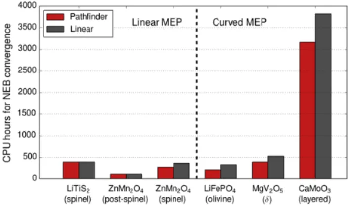
To characterize the computational efficiency gains through the PathFinder initialization, we compare the runtime of NEB calculations initialized using the PathFinder scheme versus the traditional linear interpolation. The computational resources are measured by total CPU hours used on a Cray XC30 machine with a parallelization of 24 cores per image. To ensure a fair comparison, all computational parameters are kept the same for the two initialization schemes. The results of our test are given in Fig. 8. As could be expected from our analysis of MEP geometry, initialization using the PathFinder algorithm does not significantly affect performance for structures with a linear MEP for migration, but does lead to consistent performance gains in cases where the MEP deviates from a linear path.
28
Figure 8. CPU hours used by the NEB calculations initiated from linear interpolation and PathFinder interpolation, respectively.
3.5 PathFinder v.s. Linear Interpolation on CaMoO3 example
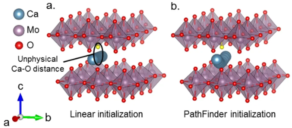
As we mentioned earlier, one of the common issues arising in NEB calculations is that linear interpolation can yield highly unphysical image structures that are difficult to relax due to exceptionally high forces and instabilities in the electronic minimization. PathFinder avoids this problem by biasing the migrating ion away from concentrations of electronic charge density, avoiding unintended reactions in the structure within intermediate images. For example, when calculating the MEP of Ca inner-layer diffusion along the a axis in CaMoO3, we find that typical NEB with linear interpolation is unstable
due to excessive forces in some images. The reason for this instability is clear from Fig. 9. Initialization of the NEB calculation from linear interpolation puts one oxygen atom (colored in yellow) too close to some of the Ca images, an issue which is avoided by the PathFinder. This unphysically small Ca-O distance results in large inter-atomic forces, destabilizing the calculation. Conventionally, such instabilities can be mitigated by careful
29
tuning of convergence and relaxation parameters needed, resulting in a significant increase in runtime and decrease in throughput. Furthermore, such instabilities are the primary reason why the NEB method has been difficult to automate and scale to thousands of compounds as is required for the newly emerging Materials Genome Database.91
Figure 9. CaMoO3 NEB calculations for Ca inner-layer diffusion. (a) Visualization of a
standard linearly-interpolated path, illustrating the unphysical Ca-O distance that arises in the middle image. Note that the problematic interacting oxygen is marked in yellow. (b)
Visualization of the PathFinder-approximated MEP, demonstrating a more physical migration path geometry that avoids the oxygen that lies near the migration path.
Chapter 4 ApproxNEB Method
While the PathFinder algorithm can provide a good approximation of the geometry of the MEP, we will demonstrate in a later section that it does not yield accurate energetics along the path. For this reason, we propose to investigate the energetics of each image using the ApproxNEB method, in which the band is decoupled into individual image calculations.
30
4.1 Methods
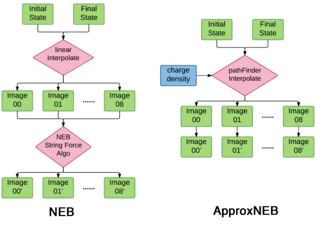
The key idea of ApproxNEB is that, if we fix the moving cation along the approximate MEP obtained from the PathFinder algorithm, and perform a single point relaxation image by image, we can acquire the missing energetics, thereby fully characterizing the MEP. The difference between ApproxNEB and NEB algorithms are depicted in Fig. 10. In general, the execution of the NEB algorithm, in first-principles or classical potential codes, requires communication between images, as they are connected by virtual springs. At the end of each ionic relaxation step, images communicate with each other to update spring forces and a new step in the constrained potential energy is taken – this procedure is repeated until the NEB force and energy criteria are satisfied. The ApproxNEB method removes the spring force and estimates the diffusion barrier by fixing the moving cation and relaxing other atoms in each image. In order to constrain translational degrees of freedom of the system, this procedure requires that the position of a reference atom that is farthest away from the moving ion in the unit cell to be fixed. This constraint prevents the whole cell from shifting uniformly to translate into the initial or final state. Under these constraints, the energy of the independently relaxed images provides an approximate MEP trajectory.
As discussed earlier, in NEB calculations, the migrating ions are relaxed by a combination of virtual spring forces and true forces, while non-migrating atoms are relaxed only by the true forces. The spring forces serve to push the migrating ions to higher energy positions on the MEP. However, if we already know the geometry of the MEP from the PathFinder
31
method, the spring forces can be removed by fixing the moving cation on the MEP. From this perspective, ApproxNEB and NEB provide equivalent constraints on the system during relaxation.
Figure 10. A comparison between traditional NEB and ApproxNEB calculation schemes. Here we assume that 7 images are interpolated between initial and final state (image 00 and image 08 are the initial and final states) and demonstrate that under the ApproxNEB scheme, image calculations are decoupled, decreasing the
32
4.2 ApproxNEB v.s. NEB on Barrier Estimation
Having established the PathFinder approach as a reliable method to efficiently estimate migration geometry, we turn to the ApproxNEB approach of charactering the energetics of the MEP. To access the validity of this approach, we compare the overall energy profile of the MEP and the migration barrier obtained from the ApproxNEB algorithm to those obtained from a traditional NEB scheme. As can be seen in Fig. 11, the two methods yield energy profiles and migration barriers within 20 meV of each other, suggesting that ApproxNEB is able to reproduce the results of NEB to good agreement across a variety of systems and migration geometries. As shown in Fig. 11b, the barriers obtained from ApproxNEB method are close to but systematically higher than those obtained from NEB. This trend is to be expected as in the ApproxNEB scheme, because the moving cation is fixed on the path provided by the PathFinder algorithm. By constraining the position of the diffusing species in each image, we reduce the degrees of freedoms available for relaxation as compared to traditional NEB, such that any error in the MEP geometry obtained from the PathFinder translates to an increase in the migration barrier. Nonetheless, just as the absolute error in the estimated MEP geometry remains within 0.2 Å across all tested systems, the error in the migration barrier remains within 20 meV, which is a sufficiently small error margin for most high-throughput screening applications where we expect this method would be of greatest interest.
33
Figure 11. (a) Minimum energy path of LiFePO4 obtained through NEB and
ApproxNEB. The absolute and relative errors of each data point on the ApproxNEB path are labeled. (b) A comparison of migration barriers obtained through NEB and ApproxNEB demonstrating a consistent agreement between the two methods within a 20 meV error bound.
4.3 ApproxNEB v.s. NEB on Computational Resource Cost
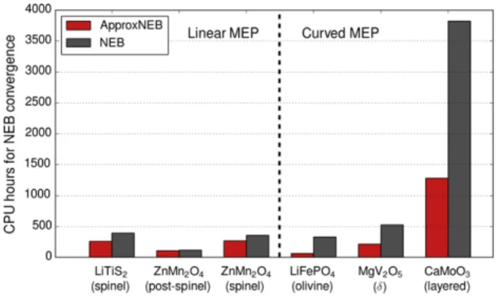
It is important to note that the computational resources necessary for ApproxNEB are substantially lower than for traditional NEB, further justifying its use in high-throughput screening applications. As can be seen in Fig. 12, for both linear and curved paths, ApproxNEB is systematically faster than the NEB method. Notably, we find that in the case of structures with curved MEP geometries, ApproxNEB yields a speedup by a factor of up to 5 with respect to linearly-initialized NEB, offering a significant improvement over even PathFinder-initialized NEB discussed earlier. The reason for this improvement lies in the decoupling of image calculations from one another. Decoupled images experience a much simpler potential field that remains quasi-static throughout the relaxation, enabling
34
efficient minima-searching during ionic relaxation. Another issue is that of parallelization - in traditional NEB, because the position of the moving cation must be communicated among images to update spring forces, every image must be fixed to be at the same ionic relaxation step (see Fig. 10). This constraint hampers the progress of the calculation because when an image converges at a certain ionic step, it has to wait for all other images to converge before the next NEB step is taken, and some computational resources are wasted during this idle phase. Finally, error handling becomes much easier for ApproxNEB. For NEB, if a calculation fails due to a convergence problem with on specific image, the whole calculation has to be restarted. Given that in ApproxNEB each image is independent, only the failed image needs to be rerun. The improvements in both computation runtime and error handling make PathFinder and ApproxNEB suitable for scaling up to screen materials properties in a high-throughput fashion.
Figure 12. CPU hours consumed by ApproxNEB and NEB methods. For the NEB method, the band is initialized from linear interpolation. However, the performance
35
gains of ApproxNEB are significantly higher than even PathFinder-initialized NEB shown in Fig. 8.
4.3 ApproxNEB Implementation
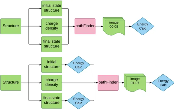
The key idea of ApproxNEB is to leverage the accurate paths predicted by PathFinder algorithm and decouple images into parallel calculations. The detailed implementation process, however, can be done in two different ways. As depicted in Fig. 13, one can either (a) start from applying PathFinder to un-relaxed start and final states and then include the calculation of two end point states in ApproxNEB, or (b) relax two end point states first, then apply the PathFinder and implement ApproxNEB at last.
Both workflows give the same reliable diffusion barrier and MEP. The CPU hours consumed by two workflows are however different. Applying two workflows to LiFePO4
system, the CPU hours consumed by workflow (b) is substantially smaller than workflow (a) (~35%). This is understandable as in workflow (b), all intermediate images can take advantages of the well relaxed end point structures as they are interpolated from them. Note that all the data in Fig. 12 (in the manuscript) are thus obtained from workflow (b) implementation strategy.
36
Figure 13. Different implementation strategy for ApproxNEB method. Note that as ApproxNEB method is indifferent to the specific first-principle software packages in use, we use “Energy Calc” in the graph to stand for the first-principle energy relaxation calculation carried out. (a) Apply PathFinder on un-relaxed structure, generate structure images including start and final states, and relax each images independently. (b) Firstly relax start and final states, then apply PathFinder to the relaxed structures, and calculate the intermediate n images independently at last.
37
Chapter 5 High-throughput ApproxNEB Framework
5.1 Error Handling
As we discussed, ApproxNEB has a huge edge over the traditional NEB method in high-throughput applications. Here we construct a simple estimate model to account for the mechanism.
Assumptions below:
• For every materials, ApproxNEB costs a of NEB time averagely (a~50%)
• Every calculation uses 7 images, every images costs the same computational power averagely.
• Every image, as itself, has a x failure rate for both ApproxNEB and NEB
• Apart from single image failure rate, NEB as a whole has a y failure rate (communication between images etc.)
• For every failure, assuming re-adjust parameters and redo can successfully converge the calculation. For ApproxNEB, we only need to redo the failure image, for NEB, we need to redo the whole calculation.
Then, for each material, assuming 𝑇 is the computational time for doing NEB once. 𝑇!""#$%&'(= 𝑎𝑇 1 + 𝑥
𝑇!"# = 𝑇 1 + 1 − 1 − 𝑥 !+ 𝑦
Depict these two functions in Fig. 14. From the graph, we can see that even though ApproxNEB only takes 1/2 of the time of NEB, but due to the fact that during error
38
handling, ApproxNEB only needs to redo failure image while NEB needs to redo the whole calculations, ApproxNEB can save 2/3 of NEB time even at x=10%
Fig. 14 Computational resources consumption, NEB v.s. ApproxNEB
5.2 EndPointFinder
A typical high-throughput application is a process shown in Fig. 15. The input database contains discharged structures, from which we know the site position of Mg in the host structures. Then we need a code module to identify the initial and final state (Fig. 13), i.e.,
39
we need a code module to automatically identify the migration starting point and ending point for a discharged Mg structure.
Fig.15, A typical Materials Science high-throughput job instance structure and
associated computation time. The middle DFT calculation step usually contains one single DFT calculation.
We call this module EndPointFinder, it's an algorithm that takes a fully discharged Mg
structure as input and output the migration initial structure, final structure and corresponding host structure for later PathFinder calculations. The algorithm workflow is shows as in Fig. 16. The basic idea is below:
• Step 1. Find all symmetrically identical Mg sties in the discharged structures • Step 2. Calculate the pair-wise distance among all Mg atoms
40
• Step 3. Classify these distance based on the initial and final Mg site symmetry properties
• Step 4. Find the shortest distance in each class of Step 3.
• Step 5. If this distance is smaller than 1.25 × 𝑠ℎ𝑜𝑟𝑡𝑒𝑠𝑡 𝑑𝑖𝑠𝑡𝑎𝑛𝑐𝑒, then this is legal migration, and corresponding inputs for PathFinder algorithm will be generated for later calculations.
41
Of course, to implement Step 1~5, we need to do some supercell scaling and shrinking, in case there is only Mg atom in a whole unit cell.
EndPointFinder turns out to be working really well, here we presented two testing examples. Fig. 17 shows the example of LiCoO2, where EndPointFinder successfully identifies the inner
layer migration pair. Fig. 18 demonstrates the example of LiFePO4, where EndPointFinder
successfully identifies the Li migration path along b axis.
Fig. 17 EndPointFinder working on LiCoO2 structure, from left to right: LiCoO2 unit cell;
LiCoO2 2×2×2 supercell, with the initial and final migration site positions identified; CoO2
42
Fig. 18 EndPointFinder working on LiFePO4 structure, from left to right: LiFePO4 unit cell,
LiFePO4 2×2×2 supercell, with the initial and final migration site positions identified; FePO4
1×1×1 supercell, the corresponding smallest host structure for the migration.
5.3 Framework
With the EngPointFinder module fully developed, we developed two high-throughput applications.
43
Fig. 18 presents the workflow of PathFinder high-throughput application, where we extract structures from the database and calculate all possible migration paths geometry using the PahFinder algorithm. Till the time writing this thesis, we’ve already calculate around 2000 migration paths.
Fig. 19 presents the workflow of ApproxNEB high-throughput applications, where EndpointFinder is followed by PathFinder and ApproxNEB method one by one. I’ve already developed this application and fully tested, but it is not put into production yet by the time I am writing this thesis.
44
Chapter 6 Conclusions and Contributions
In this thesis, I tested the high-throughput structures applying traditional NEB calculations schemes and find out it is very different to scale traditional NEB method to a high-throughput application.
Then I proposed a new scheme for estimating migration minimum- energy path (MEP) geometry and energetics (PathFinder and ApproxNEB). By testing our methodology against standard NEB calculations and literature values, we find that the PathFinder algorithm can reliably predict the geometry of cation migration MEP within 0.2 Å at negligible computational cost. Furthermore, we find that the ApproxNEB calculation scheme yields activation barriers for migration within an error bound of 20 meV while using significantly fewer computational resources than NEB. We envision that our methods can be used to accelerate NEB calculations, as well as to provide a robust estimation criterion for migration barriers in ionic materials for high-throughput computational screening of materials.
Based upon these two newly developed methods, coupled with EndPointFinder, I developed two functional high-throughput applications (ApproxNEB for estimating
45
migration barriers and PathFinder for calculating migration geometric paths), and have already put PathFinder high-throughput system into production and calculate around 2000 structures.
References
1. Thackeray, M. M., Wolverton, C. & Isaacs, E. D. Energ Environ Sci 5, 7854–7863 (2012). 2. Van Noorden, R. Nature 507, 26–28 (2014).
3. Gallagher, K. G. et al. Energ Environ Sci 7, 1555–1563 (2014). 4. Aurbach, D. et al. Nature 407, 724–727 (2000).
5. Muldoon, J. et al. Energ Environ Sci 5, 5941–5950 (2012).
6. Park, M., Zhang, X., Chung, M., Less, G. B. & Sastry, A. M. J Power Sources 195, 7904– 7929 (2010).
7. Wang, B. et al. J Electrochem Soc 143, 3203–3213 (1996).
8. Amin, R., Balaya, P. & Maier, J. Electrochem Solid St 10, A13–A16 (2007).
9. Van der Ven, A., Bhattacharya, J. & Belak, A. A. Accounts Chem Res 46, 1216–1225 (2013). 10. Van der Ven, A. & Ceder, G. Electrochem Solid St 3, 301–304 (2000).
11. Kang, K. & Ceder, G. Phys Rev B 74, 094105 (2006).
12. Morgan, D., Van der Ven, A. & Ceder, G. Electrochem Solid St 7, A30–A32 (2004). 13. Islam, M., Driscoll, D., Fisher, C. & Slater, P. Chem Mater 17, 5085–5092 (2005).
46
14. Islam, M. S. & Fisher, C. A. J. Chem. Soc. Rev. 43, 185 (2013). 15. Yoo, H. D. et al. Energ Environ Sci 6, 2265 (2013).
16. G. Mills and H. Jonsson, Phys. Rev. Lett. 72, 1124 (1994).
17. G. Mills, H. Jonsson, and G. K. Schenter, Surf. Sci. 324, 305 (1995).
18. H. Jonsson, G. Mills, and K. W. Jacobsen, in Classical and Quantum Dynamics in Condensed Phase Simulations, edited by B. J. Berne, G. Ciccotti, and D. F. Coker (World Scientific, Singapore, 1998), p.385.
19. B. Uuberuaga, M. Levskovar, A. P. Smith, H. Jonsson, and M. Olmstead, Phys. Rev. Lett. 84, 2441 (2000).
20. W. Windl, M. M. Bunea, R. Stumpf, S. T. Dunham, and M. P. Masquelier, Phys. Rev. Lett.
83, 4345 (1999)
21. R. Stumpf, C. L. Liu, and C. Tracy, Phys. Rev. B 59, 16047 (1999). 22. T. C. Shen, J. A. Steckel, and K. D. Jordan, Surf. Sci. 446, 211 (2000). 23. M. Villarba and H. Jonsson, Surf. Sci. 317, 15 (1994).
24. M. Villarba and H. Jonsson, Surf. Sci. 324, 35 (1995).
25. M. R. Sorensen, K. W. Jacobsen, and H. Jonsson, Phys. Rev. Lett. 77, 5067 (1996).
26. T. Rasmussen, K. W. Jacobsen, T. Leffers, O. B. Pedersen, S. G. Srinivasan, and H. Jonsson, Phys. Rev. Lett. 79, 3676 (1997).
47
28. R. Czerminski and R. Elber, Int. J. Quantum Chem. 24,167 (1990) 29. R. E. Gillilan and K. R. Wilson, J. Chem. Phys. 97, 1757 (1992).
30. Gregory, T. D., Hoffman, R. J., Winter, M. J. Electrochem. Soc. 137, 775–780 (1990). 31. Aurbach, D., Lu, Z.; Schechter, A., Gofer, Y., Gizbar, H., Turgeman, R., Cohen, Y., Moshkovich, M., Levi, E. Nature, 407, 724–727 (2000).
32. Levi, E., Levi, M. D., Chasid, O., Aurbach, D. J. Electroceram., 22, 13–19 (2007). 33. McKinnon, W. R., Dahn, J. R. Phys. Rev. B, 31, 3084–3087 (1985).
34. Kganyago, K. R., Ngoepe, P. E., Catlow, C. R. A. Phys. Rev. B, 67, 104103 (2003).
35. Levi, E., Lancry, E., Mitelman, A., Aurbach, D., Ceder, G., Morgan, D., Isnard, O. Chem. Mater., 18, 5492–5503 (2006).
36. Rao, C.; Biswas, K. Essentials of Inorganic Materials Synthesis. (2015)
37. Levi, E., Gershinsky, G., Aurbach, D., Isnard, O. Inorg. Chem., 48, 8751–8758 (2009). 38. Kaewmaraya, T., Ramzan, M., Osorio-Guilln, J., Ahuja, Solid State Ionics, 261, 17–20 (2014).
39. Ritter, C., Gocke, E., Fischer, C., Schollhorn, R. Mater. Res. Bull., 27, 1217–1225 (1992). 40. Levi, E., Mitelman, A., Aurbach, D., Brunelli, Chem. Mater., 19, 5131–5142 (2007).
41. Saha, P., Jampani, P. H., Datta, M. K., Okoli, C. U., Manivannan, A., Kumta, P. N. J. Electrochem. Soc., 161, A593–A598 (2014).
48
42. Lancry, E., Levi, E., Gofer, Y., Levi, M., Salitra, G., Aurbach, D. Chem. Mater., 16, 2832– 2838 (2004).
43. Schollhorn, R., Kumpers, M., Besenhard, J., Mater. Res. Bull., 12, 781–788 (1977).
44. Cheng, Y., Parent, L. R., Shao, Y., Wang, C., Sprenkle, V. L., Li, G., Liu, J. Chem. Mater.,
26, 4904–4907 (2014).
45. Geng, L., Lv, G., Xing, X., Guo, J. Chem. Mater., 27, 4926–4929 (2015).
46. Levi, E., Gershinsky, G., Aurbach, D., Isnard, O., Ceder, G. Chem. Mater., 21, 1390–1399 (2009).
47. Seghir, S., Stein, N., Boulanger, C., Lecuire, J. M. Electrochim. Acta, 56, 2740–2747 (2011). 48. Levi, M. D., Lancry, E., Gizbar, H., Lu, Z., Levi, E., Gofer, Y., Aurbach, D. J. Electrochem. Soc., 151, A1044 (2004).
49. Mitelman, A., Levi, M. D., Lancry, E., Levi, E., Aurbach, D. Chem. Commun., 4212–4214 (2007).
50. Choi, S. H., Kim, J. S., Woo, S. G., Cho, W., Choi, S. Y., Choi, J., Lee, K.-T., Park, M. S., Kim, Y. J., ACS Applied Materials & Interfaces, 7, 7016–7024 (2015).
51. Woo, S. G., Yoo, J. Y., Cho, W., Park, M. S., Kim, K. J., Kim, J. H., Kim, J. S., Kim, Y. J. RSC Adv., 4, 59048–59055 (2014).
52. I. E. Castelli, D. D. Landis, K. S. Thygesen, S. Dahl, I. Chorkendorff, T. F. Jaramillo, and K. W. Jacobsen, Energy Environ. Sci. 5, 9034 (2012).
49
53. I. E. Castelli, T. Olsen, S. Datta, D. D. Landis, S. Dahl, K. S. Thygesen, and K. W. Jacobsen, Energy Environ. Sci. 5, 5814 (2012).
54. L. Yu and A. Zunger, Phys. Rev. Lett. 108, 068701 (2012).
55. K. Yang, W. Setyawan, S. Wang, M. Buongiorno Nardelli, and S. Curtarolo, Nature Mater.
11, 614 (2012).
56. C. Ortiz, O. Eriksson, and M. Klintenberg, Comput. Mater. Sci. 44, 1042 (2009).
57. W. Setyawan, R. M. Gaume, S. Lam, R. S. Feigelson, and S. Curtarolo, ACS Comb. Sci. 13, 382 (2011).
58. L.-C. Lin, A. H. Berger, R. L. Martin, J. Kim, J. A. Swisher, K. Jariwala, C. H. Rycroft, A. S. Bhown, M. W. Deem, M. Haranczyk, and B. Smit, Nature Mater. 11, 633 (2012).
59. R. Armiento, B. Kozinsky, M. Fornari, and G. Ceder, Phys. Rev. B, 84, 014103 (2011).
60. S. Wang, Z. Wang, W. Setyawan, N. Mingo, and S. Curtarolo, Phys. Rev. X 1, 021012 (2011). 61. S. Curtarolo, W. Setyawan, S. Wang, J. Xue, K. Yang, R. H. Taylor, L. J. Nelson, G. L. W. Hart, S. Sanvito, M. BuongiornoNardelli, N. Mingo, and O. Levy, Comput. Mater. Sci. 58, 227 (2012).
62. J. Greeley, T. F. Jaramillo, J. Bonde, I. B. Chorkendorff, and J. K. Norskov, Nature Mater. 5, 909 (2006).
63. S. V. Alapati, J. K. Johnson, and D. S. Sholl, J. Phys. Chem. B 110, 8769 (2006). 64. J. Lu, Z. Z. Fang, Y. J. Choi, and H. Y. Sohn, J. Phys. Chem. C 111, 12129 (2007).
50
65. J. C. Kim, C. J. Moore, B. Kang, G. Hautier, A. Jain, and G. Ceder, J. Electrochem. Soc. 158, A309 (2011).
66. H. Chen, G. Hautier, A. Jain, C. J. Moore, B. Kang, R. Doe, L. Wu, Y. Zhu, and G. Ceder, Chemistry of Materials 24, 2009 (2012).
67. A. Jain, G. Hautier, C. Moore, B. Kang, J. Lee, H. Chen, N. Twu, and G. Ceder, J. Electrochem. Soc. 159, A622 (2012).
68. G. Hautier, A. Jain, H. Chen, C. Moore, S. P. Ong, and G. Ceder, J. Mater. Chem. 21, 17147 (2011).
69. H. Chen, G. Hautier, and G. Ceder, J. Am. Chem. Soc. 134, 19619 (2012). 70. http://pythonhosted.org/FireWorks/
71. W. E, W. Ren, and E. Vanden-Eijnden, Phys. Rev. B, 66, 052301 (2002). 72. W. E, W. Ren, and E. Vanden-Eijnden J. Chem. Phys., 126,164103 (2007).
73. M. S. Islam, D. J. Driscoll, C. Fisher, P. R. Slater, Chem. Mater., 17(20), 5085-5092 (2005). 74. https://github.com/shaunrong/NEB_PathFinder
75. S. P. Ong, W. D. Richards, A. Jain, G. Hautier, M. Kocher, S. Cholia, D. Gunter, V. L. Chevrier, K. Persson, G. Ceder, Comput. Mater. Sci., 68, 314-319 (2013).
76. H. C. Yu, C. Ling, J. Bhattacharya, J. C. Thomas, K. Thornton, A. Van der Ven, Energy Eviron. Sci., 7, 1760 (2014).
51
78. M. Liu, Z. Rong, R. Malik, P. Canepa, A. Jain, G. Ceder, K. Persson, Energy Environ. Sci., 8 (3), 964-974 (2014).
79. S. Asbrink, A. Waskowska, L. Gerward, J. S. Olsen, E. Talik, Phys. Rev. B, 60(18), 12651 (1999).
80. C. Ling, F. Mizuno, Chem. Mater. 25, 3062-3071 (2013).
81. K. Hoang, M. Johannes, Chem. Mater., 23(11), 3003-3013 (2011).
82. D. Morgan, A. Van der Ven, G. Ceder, Electrochem. Solid-State Lett., 7(2), A30-32 (2004). 83. R. Malik, A. Abdellahi, G. Ceder, J. Electrochem. Soc., 160(5), A3179-A3197 (2013). 84. R. Malik, F. Zhou, G. Ceder, Nature Materials, 10(8), 587-590 (2011).
85. S. P. Ong, C. L. Chevrier, G. Ceder, Phys. Rev. B, 83, 075112 (2011).
86. G. S. Guatam, P. Capena, R. Malik, M. Liu, K. Persson, G. Ceder, Chem. Commun., 51, 13619 (2015).
87. G. S. Guatam, P. Capena, A. Abdellahi, A. Urban, R. Malik, G. Ceder, Chem. Mater., 27(10), 3733-3742 (2015).
88. D. O. Scanlon; A. Walsh; B. J. Morgan; G. W. Watson, J. Phys. Chem. C, 112, 9903-0011 (2008).
89. C. Delmas; H. Cognac-Auradou; J. M. Cocciantelli; J. M. Menetrier; J. P. Doumerc, Solid State Ionics, 69, 257-264 (1994).
52
91. A. Jain, S. P. Ong, G. Hautier, W. Chen, W. D. Richard, S. Dacek, S. Cholia, D. Gunter, D. Skinner, G. Ceder, K. A. Persson, APL Materials, 1(1) 011002 (2013).