Publisher’s version / Version de l'éditeur: Energy and Buildings, 135, pp. 137-147, 2016-11-20
READ THESE TERMS AND CONDITIONS CAREFULLY BEFORE USING THIS WEBSITE.
https://nrc-publications.canada.ca/eng/copyright
Vous avez des questions? Nous pouvons vous aider. Pour communiquer directement avec un auteur, consultez la
première page de la revue dans laquelle son article a été publié afin de trouver ses coordonnées. Si vous n’arrivez
Questions? Contact the NRC Publications Archive team at
PublicationsArchive-ArchivesPublications@nrc-cnrc.gc.ca. If you wish to email the authors directly, please see the first page of the publication for their contact information.
NRC Publications Archive
Archives des publications du CNRC
This publication could be one of several versions: author’s original, accepted manuscript or the publisher’s version. / La version de cette publication peut être l’une des suivantes : la version prépublication de l’auteur, la version acceptée du manuscrit ou la version de l’éditeur.
For the publisher’s version, please access the DOI link below./ Pour consulter la version de l’éditeur, utilisez le lien DOI ci-dessous.
https://doi.org/10.1016/j.enbuild.2016.11.029
Access and use of this website and the material on it are subject to the Terms and Conditions set forth at
Testing the accuracy of low-cost data streams for determining
single-person office occupancy and their use for energy reduction of building
services
Newsham, Guy R.; Xue, Henry; Arsenault, Chantal; Valdes, Julio J.; Burns,
Greg J.; Scarlett, Elizabeth; Kruithof, Steven G.; Shen, Weiming
https://publications-cnrc.canada.ca/fra/droits
L’accès à ce site Web et l’utilisation de son contenu sont assujettis aux conditions présentées dans le site LISEZ CES CONDITIONS ATTENTIVEMENT AVANT D’UTILISER CE SITE WEB.
NRC Publications Record / Notice d'Archives des publications de CNRC:
https://nrc-publications.canada.ca/eng/view/object/?id=8dd905f5-6b28-4f14-9119-6435285da6a7 https://publications-cnrc.canada.ca/fra/voir/objet/?id=8dd905f5-6b28-4f14-9119-6435285da6a7
Testing the Accuracy of Low-Cost Data Streams for Determining Single-Person Office
1
Occupancy and Their Use for Energy Reduction of Building Services
2
Guy R. Newsham, Henry Xue, Chantal Arsenault, Julio J. Valdes, Greg J. Burns, 3
Elizabeth Scarlett, Steven G. Kruithof, Weiming Shen 4
5
Abstract
6
We explored methods of detecting occupancy in single-person offices using data already collected by the 7
occupant’s PC, or data from relatively cheap sensors added to the PC. We collected data at 15-second 8
intervals for up to 31 days in each of 28 offices. A combination of low/no cost sensors (webcam-based 9
motion detection, and keyboard and mouse activity) was much more accurate at detecting occupancy than 10
a commercial ceiling-based passive infrared (PIR) sensor, and provided overall daytime accuracy >90%, 11
with very low false negative rates. This enhanced detection performance would enable a reduction in the 12
timeout periods for building service curtailment on space vacancy. For example, lighting switch-off 13
timeout could be reduced from the current energy code standard of 20 minutes to less than 5 minutes, 14
increasing energy savings potential by 25-45%. We then deployed this system in a proof-of-concept 15
demonstration, using it to control lighting, heating, ventilation, and air conditioning (HVAC), and plug 16
loads in a mock-up office environment. Tests were run over nine occupied days (six in cooling season, 17
three in heating season). The system delivered energy savings of 15-68%, with no reported false negative 18
errors. 19
20 21
Glossary of Terms and Abbreviations
1
Count Total number of instances of sensor data, aggregated to the 15-second level.
TP True Positives, instances when a sensor reports a space is occupied when indeed it is. TN True Negatives, instances when a sensor reports a space is not occupied when indeed it is
not.
FP False Positives, instances when a sensor reports a space is occupied when indeed it is not. FN False Negatives, instances when a sensor reports a space is not occupied when indeed it is. Occupied (Occ) Actual fraction of time office occupied = TP/Count
Accuracy (Acc) Fraction of time a sensor correctly identifies occupancy status = (TP+TN)/Count FPR False Positive Rate =FP/(TN+FP)
FNR False Negative Rate =FN/(FN+TP)
ESR Energy savings ratio achieved by sensor system with 20-minute timeout.
MaxESR Maximum energy saving ratio by switching off lights when office is unoccupied, compared to lights being on from first arrival to last departure
2
1. Introduction
3
The key to saving energy in buildings is to deliver building services only when and where they are 4
needed, in the amount they are needed. Occupancy sensor technology and related controls have emerged 5
from this observation. Occupancy sensors have been deployed at the room level to save energy primarily 6
in ambient lighting systems [Williams et al., 2012; Galasiu et al. 2007], with the potential for energy 7
savings with HVAC systems also emerging [Dong & Lam, 2011]. Energy savings of 20-50% are 8
typically reported. 9
10
Given this success, occupancy sensors for lighting systems are now mandated in certain space types in 11
many energy codes for new buildings [e.g. CCBFC, 2011]. However, penetration of this technology as a 12
retrofit in existing buildings is low, and first-cost remains a tangible barrier. The goal of our research was 13
to lower this cost barrier by extracting free or nearly-free occupancy information from an office PC 14
platform. The attraction of a PC platform is that it is already in place in an office environment, and is 15
already powered and networked. 16
Extracting occupancy data from systems not explicitly designed to deliver occupancy information has 1
been termed “implicit occupancy sensing” [Melfi et al., 2011]. Examples of implicit occupancy data 2
include: computer network activity [e.g. Kim et al. 2010], security card access systems [e.g. Ghai et al., 3
2012], detection of mobile devices at Wi-Fi access points [e.g. Jin et al. 2014], and PC-based sources such 4
as keyboard activity, webcams, and microphones. These data streams may be supplemented by 5
environmental sensors (e.g. temperature, humidity, light, sound), which are already present in some 6
computing platforms, and are expected to become more widespread as wireless nodes lower in cost and 7
become pervasive as part of the “Internet of Things” (IoT). Although these channels might provide 8
limited accuracy in detecting occupancy independently, their aggregated data may carry more precision 9
and robustness than any one high-end sensor [Dong & Lam, 2011; Dong et al., 2010; Tiller et al., 2009; 10
Hailemariam et al., 2011; Ghai et al., 2012]. 11
12
Many studies addressing alternative means of detecting occupancy were summarized in Shen & 13
Newsham [2016]. However, few prior studies have focussed specifically on use of implicit data sources 14
and supplemental environmental sensors in single-person office spaces, with no requirement for the 15
occupant to carry hardware on their person. 16
17
Zhao et al. [2015] collected data in two offices over several weeks. Keyboard and mouse data were 18
collected every 20 seconds along with data from supplemental sensors: PIR, chair pressure, door 19
open/shut, lighting on/off, Wi-Fi connection, and GPS location. Bayesian Belief Networks were used to 20
select the optimal fusion of sensor data, which typically involved keyboard, mouse and PIR data streams. 21
Ground truth was derived from three extra PIR sensors and occupant diary entries. Overall accuracy 22
exceeded 90% 23
24
Hailemariam et al.,[2011] added light, sound, CO2, current, and motion sensors to a single office cubicle;
25
the motion sensor was mounted on the cubicle wall close to and facing the occupant. Data were 26
aggregated at the 1-minute level and collected over one week. Ground truth occupancy was obtained 27
from human transcription of video images. Using a decision-tree method, an overall detection accuracy 28
of 98% was achieved. 29
relied on a pressure sensor in the chair, a ceiling mounted PIR sensor, and two acoustic sensors (one 1
placed to register conversation and a second placed to register keyboard/mouse use). The user kept an 2
activity diary every 5 minutes to provide ground truth. A test in a single office over five days yielded 3
activity detection accuracy of 95%. 4
5
While not explicitly measuring the accuracy of an alternative occupancy sensing approach, Dalton & Ellis 6
[2003] provided a very relevant application. They used a webcam with a simple face detection algorithm 7
to determine if someone is looking at a PC display, and to switch off the display if no-one is looking at it. 8
Their very short experiments suggested display energy savings of 12-30% compared to a fixed power 9
saving mode enacted after five minutes of no PC activity. 10
11
We conducted a field study to test the accuracy of various data streams for determining the occupancy of 12
offices, and determined a combination of PC-based sensor data streams that substantially outperformed 13
the incumbent commercial technology. We then deployed the system in a full-scale demonstration to 14
control several office systems (lighting, HVAC, miscellaneous/plug loads1) over multiple test days in
15
heating and cooling seasons. This research is an advance over previous work in several important 16
aspects: 17
Data collection in more offices and over a longer time period 18
More accurate ground truth recording 19
Direct comparison to incumbent commercial technology 20
Separate consideration of false positive and false negative error types 21
Focus on accuracy during normal working hours only, when information is most relevant 22
Demonstration of actual control of building services based on the new approach 23
24
1In an office setting, these are any electrical device powered from a conventional wall socket, and may include:
computers, monitors, printers, fans, external speakers, supplemental space heaters, desk lights, coffee machines etc. [e.g. Mercier & Moorefield, 2011].
1
2. Better Occupancy Sensing
2 2.1 Methods & Procedures 3 4 2.1.1 Sensor and Data Description 5 6
We installed hardware and software on the PCs of volunteers who occupied single-person office spaces; 7
we also installed additional hardware in these offices spaces. We recorded data from a variety of different 8
sources that may indicate occupancy: 9
10
1. Keyboard and mouse activity. We recorded only if these devices had been used, not what was 11
typed or clicked. 12
2. Webcam (external retrofit2). We mathematically derived pixel value differences in consecutive
13
frames of down-sampled images3, we did not record or store images.
14
3. Microphone (external retrofit4, Phidgets 1133). We recorded only dB levels, not what was said.
15
4. Infra-red sensor (Omron D6T-44L). Low-res (4x4) pixel temperature map of the space. 16
5. Proximity sensor (MaxBotix EZ-1). Distance from sensor to nearest solid object. 17
6. Air Temperature and Relative Humidity (Phidgets 1125). 18
7. Light Level (Phidgets 1142). 19
8. PIR motion sensor (Phidgets 1111). 20
9. Commercial, PIR motion sensor (Manufacturer name/model withheld). 21
10. Pressure mat (United Security 925)5. This was used as “ground truth”.
22
2We used an external webcam because not all PCs in the study group had internal webcams, but a future low-cost
application would leverage ubiquitous internal webcams.
3Utilizing the Windows API, consecutive (40x30 pixel) images were captured every second from the webcam. The
distance in RGB space between the two images for each image pixel was calculated:
d(x, y) = ((R − R ) + (G − G ) + (B − B ) )/3
and a simple metric for motion detection was the maximum distance among all pixels.
1
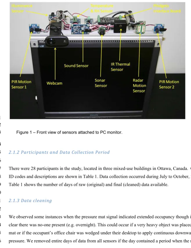
Sensors 1-8 were already present in the PC, or were mounted to the PC monitor (Figure 1); Sensor 9 was 2
mounted on the ceiling in a typical location for commercial use; Sensor 10 covered the majority of the 3
most frequently occupied floor space in the office. The external webcam was connected to the PC via a 4
dedicated USB port; other PC-based sensors that were not internal were connected to a data acquisition 5
board, and then to the PC via a single USB port6.
6 7
Data from all sensors were recorded and collated by custom software on each PC whenever the PC was 8
switched on7. Data were recorded every 15 seconds, and were a statistical summary (e.g. Counts, Max,
9
Min, Mean, Median) of raw data recorded at 1 or 5 Hz. The term “row” of data below refers to a single 10
15-second instance of data from one participant, that instance containing the statistical summary of data 11
from all sensors. 12
13
5Mat sensitivity was chosen to ensure that an empty chair or full briefcase would not trigger it.
6The radar sensor shown in Figure 1 was only installed on 15 of the sample PCs, and thus was not utilized in
further analysis.
1 2
Figure 1 – Front view of sensors attached to PC monitor.
3 4
2.1.2 Participants and Data Collection Period
5 6
There were 28 participants in the study, located in three mixed-use buildings in Ottawa, Canada. Office 7
ID codes and descriptions are shown in Table 1. Data collection occurred during July to October, 2013. 8
Table 1 shows the number of days of raw (original) and final (cleaned) data available. 9
10
2.1.3 Data cleaning
11 12
We observed some instances when the pressure mat signal indicated extended occupancy though it was 13
clear there was no-one present (e.g. overnight). This could occur if a very heavy object was placed on the 14
mat or if the occupant’s office chair was wedged under their desktop to apply continuous downward 15
pressure. We removed entire days of data from all sensors if the day contained a period when the mat 16
registered a continuous on signal for > 4 hours (considering it highly unlikely that an occupant would be 1
seated for that long). Fewer than 10% of the days in the original dataset were discarded. 2
3
We removed all weekends and public holidays to avoid diluting the dataset with long periods when non-4
occupancy would be obvious and unchallenging for any sensor to detect. We also removed the first and 5
last days of data collection for all offices. These were partial days, involving research staff 6
installing/uninstalling equipment, and not representative of normal occupancy. These two steps combined 7
resulted in about 25% of the days in the original dataset being discarded. 8
9
All rows of data (individual 15-second recordings) were removed if they occurred before the first ground 10
truth presence (mat on) signal or after the last ground truth presence signal on a given day8. This was done
11
to focus the dataset on periods of potential occupancy. Although only a small number of days of data 12
were lost at this step (about 5% of the original data set), the total number of rows in the data set was 13
almost halved. 14
15
Even after relatively conservative data cleaning choices, a large dataset remained: a total of >700,000 16
rows of 15-second data across >370 days. Further, all participants were retained in the sample, with no 17
participant contributing fewer than 8 days /14,000 rows of data. 18
19 20
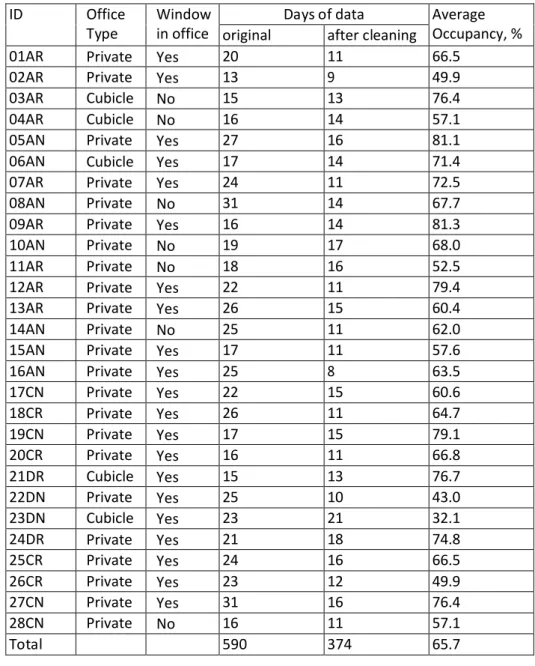
Table 1. Days of data for each office, before and after data cleaning. The final column shows the
1
percentage of time the ground truth pressure mat registered occupancy in the cleaned data set.
2
ID Office
Type Window in office original Days of dataafter cleaning AverageOccupancy, %
01AR Private Yes 20 11 66.5
02AR Private Yes 13 9 49.9
03AR Cubicle No 15 13 76.4
04AR Cubicle No 16 14 57.1
05AN Private Yes 27 16 81.1
06AN Cubicle Yes 17 14 71.4
07AR Private Yes 24 11 72.5
08AN Private No 31 14 67.7
09AR Private Yes 16 14 81.3
10AN Private No 19 17 68.0
11AR Private No 18 16 52.5
12AR Private Yes 22 11 79.4
13AR Private Yes 26 15 60.4
14AN Private No 25 11 62.0
15AN Private Yes 17 11 57.6
16AN Private Yes 25 8 63.5
17CN Private Yes 22 15 60.6 18CR Private Yes 26 11 64.7 19CN Private Yes 17 15 79.1 20CR Private Yes 16 11 66.8 21DR Cubicle Yes 15 13 76.7 22DN Private Yes 25 10 43.0 23DN Cubicle Yes 23 21 32.1 24DR Private Yes 21 18 74.8 25CR Private Yes 24 16 66.5 26CR Private Yes 23 12 49.9 27CN Private Yes 31 16 76.4 28CN Private No 16 11 57.1 Total 590 374 65.7 3
Ensuring the accuracy of ground truth was key to further analyses. Any instances when the keyboard or 4
mouse showed activity but the mat indicated no occupancy raised suspicions about the accuracy of 5
ground truth9. Only 0.17% of data rows exhibited such a data combination. We also observed some
1
ground truth state changes for only one 15-second period; i.e., a single row of non-occupancy among 2
many rows of occupancy, or vice versa. Although this behaviour might be legitimate, it might also 3
indicate a short-period lapse in correct mat functioning. From >700,000 rows of data we found only 1438 4
instances of single row state changes. Within these rows, if the mat indicated occupancy for a given 15-5
second period, but there was no keyboard or mouse activity, and both the PC-mounted motion sensors 6
and webcam recorded low levels of activity then we considered there to be a stronger case that the mat 7
had malfunctioned. This combination occurred for only 61 rows of data, or <0.01% of all rows. 8
Similarly, if the mat indicated no occupancy for a given 15-second period, but there was keyboard or 9
mouse activity, or either the PC-mounted motion sensor or the webcam recorded high levels of activity, 10
there is the possibility of malfunction. This combination occurred for only 558 rows of data, or <0.1% of 11
all rows. In summary, after initial data cleaning, residual ground truth errors are likely less than 1% of all 12
data, and it is appropriate to treat the mat data as the standard to which all other sensors are compared. 13
14
2.2 Results & Discussion
15 16
In general, in the results below, ground truth mat data has been binarized. Mat data were normalized by 17
dividing the number of readings within a 15-second period indicating occupancy by the total number of 18
readings. A value >0.5 meant the whole 15-second period was considered occupied. Only 3.6% of all 19
normalized mat recordings had a value other than 0 or 1. 20
21
Note also that although some results shown are from the entire cleaned dataset, many results are drawn 22
from the final 10% of the dataset for each office. In deriving new occupancy detection approaches, the 23
algorithm development methodology used the first 90% of the dataset for model training and the final 24
10% of the dataset for model testing. 25
26 27 28
9Although there are legitimate circumstances for such an observation – errors in the keyboard/mouse recording
2.2.1 Descriptive occupancy data based on ground truth
1 2
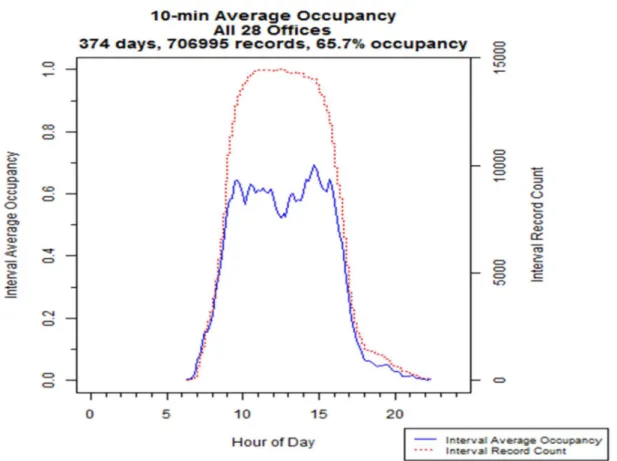
Figure 2 shows the average occupancy profile over all offices and all days. The overall occupancy rate 3
was 65.7%, with a peak of 69.3%. Occupancy exhibits a sharp rise in the morning, with a more extended 4
departure “tail” in the late afternoon. As might be expected, there is a dip in occupancy around lunch 5
time, however, this dip is not as pronounced as in other studies. This might be because work schedules at 6
the study sites were more flexible than in other office-like workplaces, or because people took some lunch 7
breaks in their office rather than another location. Table 1 also shows the mean occupancy for each 8
office. There was considerable variation across offices and days, suggesting that we captured a wide 9
range of schedules and job types in our study sample. 10
11
These observations are broadly in line with office occupancy profiles measured in other studies. For 12
example, Rubinstein et al. [2003] used traditional occupancy sensors in 35 private offices to record 13
occupancy every minute over a year (1999) in a large office building in San Francisco. Profiles on the 14
two study floors showed a similar shape to Figure 2, with occupancy peaked at ~75% and ~80%, 15
respectively. Duarte et al. [2013] used data from 629 PIR occupancy sensors in a large multi-tenant 16
office building in Boise, Idaho. Data were collected over two years (2009-2011) and collated at the 1-17
minute level. The average profile for private offices was similar to Figure 2, with a peak occupancy of 18
~50%. Yang & Becerik-Gerber [2014] collected occupancy data from 28 private offices in a university 19
office building in southern California. Occupancy was determined from a combination of sensors. They 20
developed personalized occupancy forecasts, with peak occupancy typically 60-70%. Zhao et al. [2014] 21
measured occupancy using wearable devices and PC activity data in 15 open-plan university offices over 22
three months in 2013. The average weekday had peak occupancy ~68%. D’Oca & Hong [2015] recorded 23
occupancy at 10-minute intervals in 16 private or semi-private offices in Germany over two years. They 24
sought clusters of occupancy profiles rather than a single average, but three of four cluster profiles had a 25
similar overall pattern to Figure 2, with a peak occupancy 60-65%. 26
Figure 2 – The blue line (primary y-axis) shows occupancy averaged over all offices and all days, at 10-minute time resolution. The red line (secondary y-axis) shows the total number of data points contributing to each 10-min bin. (entire dataset).
1
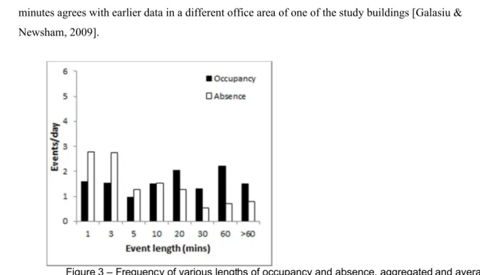
Next, we examined the frequency of various lengths of occupancy and absence, aggregated across all 2
offices and days, as shown in Figure 310. For practical control to save energy, it is the longer events that
3
have a greater importance. The number of around five absences per day for absences longer than five 4
10Our first look at these data showed that the frequency of very short events was high and could have been
inflated by non-genuine single row state changes (described above). To correct for this potential (and minor) ground truth error, we ran a script that (temporarily) modified the binarized ground truth value: a single row state change was recoded to match the state of the rows on either side, so a sequence of 11110111, became 11111111, and so on. This was done for these frequency calculations only, and not for the analyses in other sections.
minutes agrees with earlier data in a different office area of one of the study buildings [Galasiu & 1
Newsham, 2009]. 2
3
Figure 3 – Frequency of various lengths of occupancy and absence, aggregated and averaged across all offices and days. Event length 1 = events of less than 1 minute duration, Event length 3 = events between 1 and 3 minutes duration, and so on. (entire dataset).
4
From these data we made initial estimates of energy savings potential, if building systems were controlled 5
based on ground truth data. We considered savings for switching lighting systems limited to fully on and 6
fully off states. Lighting is straightforward in that it obviously only needs to be on during occupancy. 7
Savings for plug loads might be considered similar to lighting, although some plug loads (e.g. those based 8
on electronics) might need to be maintained in a partial-off state to facilitate appropriate restart when the 9
occupant returns. HVAC savings are more complex, as pre-conditioning prior to occupancy is needed to 10
avoid comfort penalties. 11
12
The theoretical maximum lighting energy savings assume lighting is switched off immediately upon 13
detecting vacancy, and switched back on again immediately when detecting occupancy11. However, any
14
inaccurate detection of vacancy (false negatives) results in lights switching off with an occupant in the 1
space, causing substantial dissatisfaction. Therefore, lighting control systems typically employ a safety 2
factor, or timeout period, such that vacancy must be detected continuously for a given period before lights 3
are switched off. Current energy codes specify a maximum timeout period for occupancy control of 30 4
minutes, with new code revisions lowering this to 20 minutes [ASHRAE, 2010; CCBFC, 2011]. In Table 5
2 below we present calculated savings for various timeout periods, based on our ground truth data, 6
aggregated across all offices and days. These calculations show that savings may increase substantially if 7
the timeout period is reduced, as has long-been recognised (e.g. Von Neida et al. [2001]; Richman et al. 8
[1996]; Maniccia et al. [2001]; Dikel & Newsham [2014]). This signals the potential for additional 9
savings with more reliable methods of detecting occupancy that allow timeout periods to be lowered 10
without elevating the risk of false negatives. 11
12
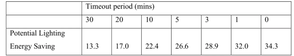
Table 2. Calculated lighting energy savings (%) based on ground truth data, aggregated across all
13
offices and days, for various timeout periods.
14
Timeout period (mins)
30 20 10 5 3 1 0 Potential Lighting Energy Saving 13.3 17.0 22.4 26.6 28.9 32.0 34.3 15 2.2.2 Ceiling-based PIR sensor as comparison 16 17
Although our PIR installations were not optimized for each office, we submit that this is also true for 18
commercial installations. However, in a commercial installation poor performing set-ups would likely be 19
remedied12. Therefore, it may be more appropriate to compare a new sensor approach to the
better-20
performing ceiling PIR installations, rather than the average. 21
22
calculations we will consider the “worst case” situation of a space without other light sources.
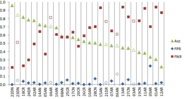
Figure 4 shows the performance of the ceiling PIR sensor compared to ground truth (mat) in each office 1
individually13and at the 15-second level. The results show a wide range of performance across offices.
2
False positives were relatively few. Overall accuracy was poor, as a result of the very high rate of false 3
negatives, in other words, in many PIR installations the sensor did not reliably “see” the seated occupant 4
for the majority of occupied time. Despite their growing deployment, few studies have looked at the 5
accuracy of PIR sensors in actual installations, and those that have often observe disappointing 6
performance. For example, in the studies quoted by Williams et al. [2012] the savings from actual 7
installations, although frequently conducted in highly-curated environments, were on average 25% lower 8
than those from simulations. Tiller et al. [2010] observed very different sensing accuracy from three 9
identical occupancy sensors installed on three walls of the same office, and all sensors reported 10
substantially lower occupancy than ground truth (human observers). NLPIP [1998] performed extensive 11
laboratory testing of occupancy sensors from multiple vendors, using a robotic arm to test the response of 12
the sensors to motion within the claimed sensor coverage area. They found many sensors unresponsive to 13
small- and medium-sized motion triggers. Priyadarshini & Mehra [2015] also note the PIR sensors are 14
relatively insensitive to motion that is not perpendicular to the direction of view of the sensor, and that 15
they are particularly prone to false negatives. 16
17
13
Figure 4 – Performance of the ceiling PIR sensor compared to ground truth (mat) in each office individually, at the 15-second level (i.e. no timeout). Offices rank-ordered by overall accuracy. Unfilled symbols indicate cubicle offices. (10% testing data).
1
Table 3 shows the effect of various timeout period lengths on ceiling PIR performance metrics for all 2
offices collectively (count-weighted). It also indicates a dramatic reduction in FNs with increasing 3
timeout, associated with a dramatic increase in FPs (because any timeout period added after a genuine 4
departure is considered as a false positive occupancy). 5
6
Table 3. Ceiling PIR metrics for various timeout periods (0 min timeout indicates15-second data).
7
(10% testing data).
8
Timeout period (mins)
All offices 30 20 10 5 3 1 0
Acc 0.7363 0.7516 0.7585 0.7430 0.7178 0.6527 0.5593 FPR 0.6518 0.5490 0.3980 0.2746 0.2069 0.1077 0.0275 FNR 0.0554 0.0871 0.1574 0.2475 0.3227 0.4759 0.6626 9
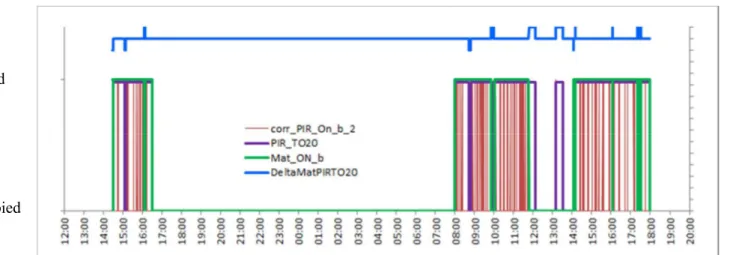
Figure 5 illustrates the effect of the 20-minute timeout for a single example office. The 15-second PIR 10
data features many FNs (Tiller et al. [2010] report similar data at the 1-second level), and an FP episode 11
(around 13:10 on the second day). Application of the 20-minute timeout to the PIR data eliminates most 1
FNs, but introduces more FPs. 2 3 Occupied Unoccupied FP FN
Figure 5 – Typical data set for office 19CN, showing raw 15-second data (green: ground truth; red: PIR response), the application of a 20-minute timeout to the PIR data (purple), and the resulting errors vs. ground truth (blue). (10% testing data).
4
This analysis provides guidelines for performance targets for an alternative sensor package. False 5
negatives represent the biggest barrier to satisfactory technology adoption, therefore, the false negative 6
ratio (FNR) is our primary performance target. Given current North American energy codes, a maximum 7
timeout period of 20 minutes is allowable for incumbent technology. Therefore, we propose that the 8
appropriate target FNR for an alternative sensor package should be that achieved by the ceiling-based PIR 9
motion sensors with a 20-minute timeout – the goal is that the alternative sensor package achieves this 10
FNR with a shorter timeout, thus enhancing energy savings. Given the discussion above we propose 11
using the upper quartile of the seven offices with the best performing PIRs, chosen according to their 12
overall accuracy following the application of a 20-minute timeout, to provide the FNR target. 13
14
2.2.3 Choice of alternative/implicit occupancy sensors
15 16
We began by comparing the accuracy of each sensor’s output vs. ground truth. This simple analysis 17
indicated that the webcam was a good single indicator of occupancy. The PC-mounted motion sensor and 18
overall. The mouse and keyboard were not good performers by themselves, although they deliver no FPs, 1
they cannot detect the presence of someone doing something other than computer work; this suggests they 2
might be good in combination with another sensor. 3
4
Many advanced analysis methods and sensor combinations were possible. We chose to focus on “good 5
enough”, parsimonious methods that were easily interpretable, using sensor packages that are low-cost 6
and practical. Thus, we chose keyboard+mouse+webcam representing sensors already in place for most 7
new computing platforms14.
8 9
2.2.4 Data fusion with genetic programming
10 11
Machine learning and computational intelligence provides a wide variety of approaches for data-driven 12
model discovery [Solomatine & Ostfeld, 2008]. We performed initial experiments using decision trees 13
and random forests, but focused on genetic programming (GP) [Koza, 1989, 1992, 1994], which has been 14
successfully applied to a wide variety of fields (e.g., to generate new integrated circuits, antennas and 15
controllers in circuit design [Koza et.al, 2003]). The variant of GP used here is Gene Expression 16
Programming (GEP) [Ferreira, 2001, 2006]. Consequently, models emerged from a two-stage process: (i) 17
a computational intelligence data driven model learning phase, and (ii) a model selection phase 18
determined by criteria specified by human experts with application domain knowledge. The specific tool 19
used in stage (i) was described in Valdés et al. [2007]. 20
21
The first 90% of the timespan of data from each office was used as a training dataset, with the remaining 22
10% (typically around 1.5 days per office) as a testing dataset; results are reported based on performance 23
against the testing dataset. For each sensor in our candidate sub-set (normalized, standardized) min, max, 24
mean, and standard deviation metrics for each 15-sec timestep were potential predictors, with no 25
interaction terms. 26
27
14We also explored an option with an additional, PC-mounted motion sensor. However, overall, the additional
The evolutionary process started with a randomly generated population of candidate functions. Many 1
different genetic operators were applied in each generation, including mutation, recombination, inversion, 2
and transposition. The particular individual (analytical function model) affected by the operator, and 3
which part of its chromosome was affected, was determined randomly according to a collection of 4
probabilities applied to the genetic operators. 5
6
In each run, the population size was fixed at 30 individuals, which were modified over 1000 generations. 7
Up to 8 genes (function terms) were allowed per individual, the function set within genes that operated on 8
predictors was limited to {+, -, *, ^2} and genes were linked by simple addition. We conducted 4500 9
such runs, using different fitness criteria (e.g. based on resulting overall accuracy, FNs, FPs) across these 10
runs, and chose the best performing function at the end of each run. This generated a list of 4500 11
candidate functions. The final models were picked by rank-ordering these candidate functions according 12
to application-relevant performance parameters, in particular FNs, and also according to the simplicity of 13
the function, judged by a domain expert. 14
15
The final model chosen was designated #2043, shown below. 16 17 Model #2043: 18 14.54+3*z_Keyboard_ON_n+4*z_Mouse_ON_n+z_WebCam_Max+z_WebCam_StdDev 19 (threshold = 9.0) 20 21
where, the prefix “z_” indicates a standardized value, and the suffix “_n” indicates a normalized value. If 22
the model yields a value greater than the threshold at a given timestep then occupancy is predicted. 23
Note, a further simplification of the function might be possible by combining the data from the keyboard 24
and mouse into a single data channel representing “tactile interaction with the computer”. Whether this is 25
effective, without negatively affecting the overall accuracy, is a topic for future work. 26
27
2.2.5 Ceiling PIR vs. alternative sensor performance
28 29
Model #2043 had an overall accuracy on 15-sec data >90%, substantially better than the overall accuracy 30
of the ceiling PIR sensors. To estimate the enhanced energy saving potential compared to the upper 31
timeout (Table 4, 0.0064) and for each office looked at the timeout needed with Model #2043 to achieve 1
the same FNR. We did this for all 28 offices, and for the 7 upper quartile PIR offices. 2
3
Table 4 compares overall performance metrics for ceiling PIR and Model #2043. The superior 4
performance of the new occupancy sensing system is clear, with substantially improved accuracy and 5
higher energy savings potential over a PIR with 20-minute timeout, even in offices representing the upper 6
quartile of PIR performance. The only metric where Model #2043 performed worse is average FNR for 7
the upper quartile offices. This is because there is one office in seven where Model #2043 performs less 8
well than the PIR, and this performance is poor enough (FNR>9%) that its inclusion in the average drags 9
down the average overall. Average performance of Model #2043 in the other six offices is much better 10
(Acc.=0.9221; FPR=0.0194; FNR=0.0037, and timeout <1 min.). 11
12 13
Table 4. Key performance metrics for PIR sensors with a 20-min timeout, and for Models #2043 with
1
a timeout chosen in each office to yield an FNR <= 0.0064. (10% testing data).
2
PIR Model #2043
All 28 offices Offices in PIR
Upper quartile All 28 offices
Offices in PIR Upper quartile
Mean Timeout (mins) 20 20 8.7 4.6
Accuracy 0.7516 0.8872 0.8812 0.9507 FPR 0.5490 0.3635 0.2919 0.1117 FNR 0.0871 0.0064 0.0258 0.0228 Actual Occupancy 0.6507 0.7020 0.6507 0.7020 ESR, % 21.4 19.4 26.4 28.1 MaxESR 0.613 0.652 0.756 0.942 3
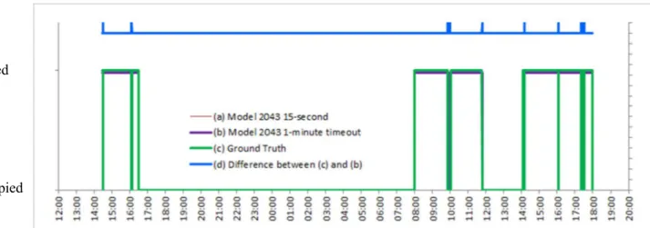
Figure 6 illustrates the effect of the 1-minute timeout on Model #2043 for the same example office in 4
Figure 5. In this case, the 15-second data was virtually coincident with the ground truth. This indicates a 5
much more accurate occupancy sensing system than with the PIR. With a 1-minute timeout applied to 6
Model #2043 in this office all FNs were eliminated. And the better sensing accuracy and reduced timeout 7 resulted in fewer FPs. 8 Occupied Unoccupied FP FN
Figure 6 – Typical data set for office 19CN, showing raw 15-second data (green: ground truth; red: Model 2043), the application of a 1-minute timeout to the Model 2043 data (purple), and the resulting errors vs. ground truth (blue). (10% testing data).
We also explored occupancy detection models that did not use the webcam in order to investigate the 1
trade-off between privacy gain and performance loss. Instead of the webcam we used the PC-mounted 2
motion sensor. Derived Model #2494 yielded acceptable accuracy and parsimony. Its performance at the 3
15-sec data level compared to the earlier models with the webcam, and to the ceiling PIR sensor, is shown 4
in Table 5. However, although the motion sensor does not have the same privacy concerns as the 5
webcam, unlike the webcam, a motion sensor is not present in most PC systems, thus it would carry a 6
small incremental cost. 7 8 Model #2494: 9 9.68+5*z_Mouse_ON_n+2*z_Motion1_Max+2*z_Keyboard_ON_n 10 11
Table 5. Performance of Models #2043 and #2494 vs. ceiling PIR, at the 15-sec data level, over all
12
offices. (10% testing data).
13
Model number PIR #2043 #2494 Accuracy 0.9023 0.8857 0.5593 FPR 0.0975 0.1130 0.0275 FNR 0.0978 0.1150 0.6626 14 3. Control Demonstration 15 3.1 Methods & Procedures 16 17
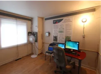
We deployed Model #2043 occupancy detection in a proof-of-concept demonstration, linking it to the 18
control of various building services and equipment in a mock-up office environment (Figure 7). 19
Colleagues were invited to occupy the test office for one full day. They were free to work on whatever 20
tasks they wished. Participants were encouraged to bring their own laptop on which the occupancy 21
sensing algorithm and control software were installed15.
22 23
Figure 7. Test office within where control proof-of-concept was performed.
1
We deployed a variety of timeout and restoration conditions to different devices under control, as shown 2
in Table 6. We covered the window in the test space with a blind to ensure that the electric lighting 3
would be needed during occupancy, but residual daylight was sufficient for basic visibility if electric 4
lighting was off. To limit the potential for FPs generated by large changes in daylight, we required the 5
model to predict a majority in five contiguous 15-second samples to indicate occupancy before the system 6
went into occupied mode. However, to allow for instant-on for the plug loads we implemented an 7
override to Model #2043, which allowed for occupancy detection at the 5 Hz sampling rate for mouse and 8
keyboard activity, or very large changes in the webcam pixel values, when the prior detected condition 9
was no occupancy. Timeout criteria (to avoid FNs) were applied following the last detected occupancy in 10
order to shift the system into vacant mode. 11
12
Table 6. Devices under control, and their timeout and service restoration condition.
13
OFF timeout (mins) ON, restoration condition Measured power draw (W)
Light 2 Manual 80
Monitor 4 Instant 15
Thermostat (setback) 5 After 1 min. occupancy n/a
Control of the light, thermostat, and plug loads were actuated via an Insteon wireless network, in which 1
control signals generated from Model #2043 were relayed via a USB dongle on the occupant’s laptop to 2
remote Insteon devices (dongle – 2448A7, light switch – part # 2477S, thermostat – part # 2441TH, 3
recessed smart plug – part # 2663-222). Control of the supplementary computer monitor was achieved 4
via the WindowsTMinternal API.
5 6
We installed additional equipment to provide a physical confirmation of the specified control actions, 7
including a temperature sensor, light sensor and clamp-on plug load sensor (manufactured by Phidgets). 8
The plug load sensor measured the current on the controlled circuit which supplied both the fan and 9
supplementary computer monitor. The temperature sensor was positioned at the HVAC supply outlet in 10
the test office floor. Participants were asked to comment on any FNs or FPs they observed, during 11
occupancy, or after returning from a period of absence, respectively. 12
13
3.2 Results & Discussion
14 15
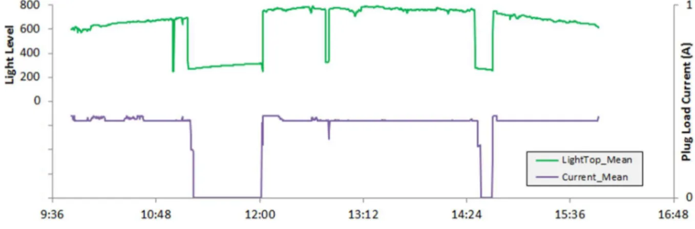
Figure 8 shows an example of the data from one summer test day. There were two periods of extended 16
vacancy, one beginning around 11:00, and the second around 14:30. There were a few very short periods 17
where the system also recorded no occupancy, and the participant confirmed these to be accurate. Also, 18
there were no short spikes in occupancy during longer vacancy periods that are indicative of FPs. 19
Figure 8. Data from September 4th, 2015. Lower chart shows occupancy as detected by Model #2043, and the switch status transmitted to the light switch and smart plug (left y-axis, any value >0 indicates “on”). This chart also shows the cooling mode setpoint transmitted to the thermostat, the local air temperature reported by the thermostat, and the temperature (“Temp2”) at the HVAC supply outlet (right y-axis). Upper chart shows the horizontal light level recorded in the office (left y-axis), and the current measured on the controlled smart plug (right y-axis).
1
As designed, the thermostat in cooling mode went to its setback temperature of 25 oC five minutes after
2
occupancy was no longer detected. This switched off the air conditioner, such that the air temperature 3
measured at the HVAC supply outlet rose rapidly; this was quickly reversed when occupancy was 4
restored16. The measured light level reflected the recorded occupancy and associated control signals
5
faithfully. Drops in light level (down to the level provided by residual daylight) as the electric lighting 6
was switched off during the longer periods of vacancy were obvious. Because the light switching had the 1
shortest timeout period (2 minutes), there were also some short duration light level drops associated with 2
the reported shorter-term absences17. The measured current also followed the occupancy and related
3
sensor signals as expected. Four minutes after occupancy was no longer detected, the current dropped 4
from 0.4 A to 0.25 A when the monitor was switched off. Two minutes later, the fan plug load was 5
turned off, and the current dropped to 0 A. 6
7
The dates and times of the various test days are shown in Table 7, along with the measured energy 8
savings compared to an uncontrolled setting. The energy savings obviously depend heavily on the 9
individual occupancy schedules on any given day, but the percentage savings were substantial, ranging 10
from 15-68%18.
11 12
Table 7. Test days for the algorithm-based occupancy detection system to control various building
13
services, and the resulting energy savings.
14
Participant Date Time Span (approx.) HVAC mode Energy Saving, %*
Lighting Plug Load** HVAC***
01 2015-07-21 0900-1700 Cool 59.6 46.6 51.9 02 2015-08-12 1400-1630 Cool 51.9 48.3 33.7 03 2015-09-02 1000-1630 Cool 31.5 30.4 30.9 04 2015-09-04 1000-1600 Cool 20.0 15.6 16.6 05 2015-09-08 1100-1600 Cool 36.6 33.8 26.1 06 2015-09-09 0930-1600 Cool 60.6 47.3 48.4 07 2015-12-17 0930-1600 Heat 25.3 21.2 22.6 08 2015-12-18 0900-1630 Heat 37.5 35.7 36.3 09 2015-12-22 1000-1830 Heat 67.8 63.0 63.9
* Calculated over period from first occupancy to last occupancy or plug load timeout, whichever comes last,
15
compared to always on during occupancy.
16
** Slightly conservative in energy terms as this assumes the 6 min. fan timeout, whereas the monitor is also
17
controlled on the same plug with a slightly shorter, 4 min. timeout.
18
*** Savings only counted if furnace not calling for heat/cool during setback.
19
17The residual daylight leaking around the blind imposed a time-dependent pattern on the total light level. 18The energy use of the sensor system itself was minimal, with a power draw < 2W, so inconsequential compared
1
4. General Discussion on Deployment Scale-up
2
This study demonstrated great potential to employ data sources not currently used to detect office 3
occupancy to accurately indicate occupancy, and thus to support building control optimization and 4
enhance energy saving opportunities. Nevertheless, the work was limited to single-person offices with 5
static computing platforms. There are several issues to be considered when contemplating broader 6
application in offices. Among these are: 7
Multi-person, open-plan offices: in a shared office space the keyboard and mouse data would 8
remain accurate and associated with the person assigned to a specific desk. However, at any one 9
desk there would be substantial background webcam activity due to the presence of other 10
occupants in and around other desks. This would likely lower the accuracy of algorithms based 11
on our current methods, with particular risk to increasing false positives. More sophisticated 12
webcam data processing may be necessary. Testing in such a context should be explored in 13
future research. 14
Mobile computing: in many workplaces mobile laptops, tablets and other computing devices are 15
displacing traditional, fixed computing platforms. As long as these are associated with the desk 16
and associated systems in the office they are being used in, and as long as they have input devices 17
equivalent to a keyboard and mouse and have a webcam, our approach should work. Of course, 18
our approach only works while a fixed or mobile computing device with these properties is 19
active. Workplaces in which computing devices are absent/off will require another occupancy 20
detection method. 21
Building system integration: in our work we customized the integration between the occupancy 22
detection method and the controlled building systems. Protocols to integrate IT and building 23
automation systems (BAS) are not yet seamless, and industry developments in this direction are 24
required if buildings are to take full advantage of the coming IoT. Common to all advanced 25
control systems, on-going maintenance of software, user databases etc. is essential to long-term 26
success. 27
Privacy: in one sense, this technique does not infringe further on privacy than already-accepted 28
methods of occupancy detection. Energy codes require occupancy sensors for lighting control in 29
single-person offices already, and to the systems that support conventional sensors thus indicate 30
visible beyond the state of the lighting in the office itself. However, our method utilizes a 1
webcam, and requires the camera to be on constantly. Although the pixel resolution required can 2
be downgraded such that most actual privacy issues are not relevant, the perceived privacy 3
concerns might be more difficult to assuage. In such cases people may resort to taping over 4
webcams as they tape over conventional occupancy sensors when they do not provide the desired 5
functionality. Nevertheless, technology and associated applications are continuing to eat away at 6
the level of continuous visual monitoring and social norms are changing, and continuously-7
recording media devices might become commonplace for other reasons. 8
9
5. Conclusions
10
These results suggest that there is great potential to leverage currently unused data sources to support 11
building controls and enhance energy saving opportunities. This offers a very cost-effective way for 12
energy-efficiency in buildings to be increased, especially in retrofit scenarios. Such opportunities are 13
likely to grow as the “Internet of Things” propagates and the density of data gathering devices in the built 14
environment increases dramatically. 15
16
Specifically, a combination of keyboard/mouse activity and pixel changes in a webcam image proved to 17
be a much better occupancy sensor than incumbent commercial technology (ceiling-based PIR). More 18
effective occupancy sensing supports shorter timeout periods for lighting (and plug load and HVAC) 19
control, leading to savings potentially 25-45% higher than current energy code controls. 20
21
Subsequent testing of this approach in a full-scale proof-of-concept demonstration in a mock-up office 22
delivered perfect occupancy sensing and energy savings of 15-68% on lighting, HVAC, and plug loads. 23
24
6. Acknowledgments
25
This work was funded by the ecoENERGY Innovation Initiative (EcoEII) administered by Natural 26
Resources Canada (NRCan), by the National Research Council Canada, and the Conservation Fund of the 27
Independent Electricity System Operator (formerly Ontario Power Authority). We are grateful to the 28
building occupants who consented to allowing us to collect data in their offices. 29
1
7. References
2
ASHRAE. 2010. ANSI/ASHRAE/IES Standard 90.1-2010 (I-P Edition), in Energy Standard for 3
Buildings Except Low-Rise Residential Buildings, ASHRAE: Atlanta, GA. 4
5
CCBFC. 2011. Canadian Commission on Building and Fire Codes (CCBFC), National Energy Code of 6
Canada for Buildings (1st ed.), 2011, National Research Council of Canada: Ottawa, ON. 7
8
Dikel, E.E.; Newsham, G.R. 2014. A quick timeout: unlocking the potential energy savings from shorter 9
time delay occupancy sensors. LD+A (December), pp. 54-56. 10
11
D'Oca, S.; Hong, T. 2015. Occupancy schedules learning process through a data mining framework. 12
Energy and Buildings, 88, pp. 395-408. 13
14
Dong, B; Lam, K.P. 2011. Building energy and comfort management through occupant behaviour 15
pattern detection based on a large-scale environmental sensor network. Journal of Building Performance 16
Simulation, 4 (4), pp. 359-369. 17
18
Ferreira, C. 2001. Gene expression programming: a new adaptive algorithm for problem solving. Journal 19
of Complex Systems, 2, pp. 87-129. 20
21
Ferreira, C. 2006. Gene Expression Programming: Mathematical Modeling by an Artificial Intelligence. 22
Springer, Studies in Computational Intelligence, 21. 23
24
Galasiu, A.D.; Newsham, G. R.; Suvagau, C.; Sander, D. M. 2007. Energy saving lighting control 25
systems for open-plan offices: a field study. Leukos 4 (1), pp. 7–29. 26
27
Galasiu, A.D., Newsham, G.R. 2009. Energy savings due to occupancy sensors and personal controls: a 28
pilot field study, Lux Europa 2009, 11th European Lighting Conference (Istanbul, Turkey), pp. 745-752 29
Ghai, S.K.; Thanayankizil, L.V.; Seetharam, D.P.; Chakraborty, D. 2012. Occupancy detection in 1
commercial buildings using opportunistic context sources. Proceedings of PerCom (Lugano), pp. 469-2
472. 3
4
Hailemariam, E.; Goldstein, R.; Attar, R.; Khan, A. 2011. Real-time occupancy detection using decision 5
trees with multiple sensor types. Proceedings of SimAUD 2011 (Boston), pp. 23-30. 6
7
Jin, M.; Jia, R.; Kang, Z.; Konstantakopoulos, I.; Spanos, C. 2014. PresenceSense: zero-training 8
algorithm for individual presence detection based on power monitoring. Proceedings of the 1st ACM 9
International Conference on Embedded Systems for Energy-Efficient Buildings (BuildSys’14) (Memphis, 10
TN), pp. 1-10. 11
12
Kim, Y.; Balani, R.; Zhao,H.; Srinivastava, M. 2010. Granger causality analysis on IP traffic and circuit-13
level energy monitoring. Proceedings of the 2nd ACM Workshop on Embedded Sensing Systems for 14
Energy-Efficiency in Buildings (BuildSys 2010), pp. 43-48. 15
16
Koza, J.R. 1989. Hierarchical genetic algorithms operating on populations of computer programs. 17
Proceedings of the 11thInternational Joint Conference on Artificial Intelligence (Detroit, USA), 1, pp
18
768-774. 19
20
Koza, J.R. 1992. Genetic Programming: On the Programming of Computers by Means of Natural 21
Selection. MIT Press. 22
23
Koza, J.R. 1994. Genetic programming II : Automatic Discovery of Reusable Programs. MIT Press. 24
25
Koza J.R.; Keane M.A.; Streeter M.J. 2003. What’s AI Done for Me Lately? Genetic Programming’s 26
Human-Competitive Results. IEEE Intelligent Systems, 18 (3), pp. 25-31. 27
28
Maniccia, D.; Tweed, A.; Bierman, A.; Von Neida, B. 2001. The effects of changing occupancy sensor 29
timeout setting on energy savings, lamp cycling and maintenance costs. Journal of Illuminating 30
Engineering Society, 30(2), pp. 97-110. 31
Melfi, R.; Rosenblum, B.; Nordman, B.; Christensen, K. 2011. Measuring building occupancy using 1
existing network infrastructure. Proceedings of the International Green Computing Conference 2
(Orlando), 8 pages. 3
4
Mercier, C.; Moorefield, L. 2011. Commercial Office Plug Load Savings and Assessment. California 5
Energy Commission, PIER Energy-Related Environmental Research Program. CEC-500-08-049. Ecos 6
Consulting. 7
8
National Lighting Product Information Program (NLPIP). 1998. Occupancy Sensors: Motion Sensors for 9
Lighting Control. Lighting Research Center, Troy, NY, USA. 10
11
Nguyen, T.A.; Aiello, M. 2012. Beyond indoor presence monitoring with simple sensors. Proceedings of 12
the 2nd International Conference on Pervasive Embedded Computing and Communication Systems 13
(Rome, Italy), pp. 5-14. 14
15
Priyadarshini, R.; Mehra, R.M. 2015. Quantitative review of occupancy detection technologies. 16
International Journal of Radio Frequency Design, 1 (1), pp. 1-19. 17
18
Richman, E.E.; Dittmer, A.L.; Keller, J.M. 1996. Field analysis of occupancy sensor operation: 19
parameters affecting lighting energy savings. Journal of the Illuminating Engineering Society, 25(1), pp. 20
83-92. 21
22
Rubinstein, F.; Colak, N.; Jennings, J.; Neils, D. 2003. Analyzing occupancy profiles from a lighting 23
controls field study. Proceedings of the 25th Session of the CIE (San Diego), 2, pp. D3-162 to D3-165. 24
25
Shen, W.; Newsham, G. 2016. Implicit Occupancy Detection for Energy Conservation in Commercial 26
Buildings: A Review. Proceedings of IEEE 20th International Conference on Computer Supported 27
Cooperative Work in Design (IEEE CSCWD 2016) (Nanchang, China), pp. 625-631. 28
29
Solomatine, D.P and Ostfeld, A. 2008. Data-driven modelling: some past experiences and new 30
Tiller, D.K.; Guo, X.; Henze, G.P.; Waters, C.E. 2009. The application of sensor networks to lighting 1
control. Leukos, 5 (4), pp. 313-325. 2
3
Tiller, D.K.; Guo, X.; Henze, G.P.; Waters, C.E. 2010. Validating the application of occupancy sensor 4
networks for lighting control. Lighting Research & Technology, 42(4), pp. 399-414. 5
6
Valdés, J.J.; Barton, A.J; Orchard R. 2007. Virtual Reality High Dimensional Objective Spaces for 7
Multi-objective Optimization: An Improved Representation. I Proceedings of EEE Congress on 8
Evolutionary Computation (Singapore), pp. 4191-4198. 9
10
Von Neida, B.; Maniccia, D.; Tweed, A. 2001. An analysis of the energy and cost savings potential of 11
occupancy sensors for commercial lighting systems. Journal of Illuminating Engineering Society, 30(2), 12
pp. 111-122. 13
14
Williams A.; Atkinson B.; Garbesi K.; Page E.; Rubinstein F. 2012. Lighting controls in commercial 15
buildings. Leukos 8(3), pp. 161-180. 16
17
Yang, Z.; Becerik-Gerber, B. 2014. The coupled effects of personalized occupancy profile based HVAC 18
schedules and room assignment on building energy use. Energy and Buildings, 78, pp. 113-122. 19
20
Zhao, J.; Lasternas, B.; Lam, K.P.;Yun, R.; Loftness, V. 2014. Occupant behavior and schedule 21
modeling for building energy simulation through office appliance power consumption data mining. 22
Energy and Buildings, 82, pp. 341-355. 23
24
Zhao, Y.; Zeiler, W.; Boxem, G.; Labeodan, T. 2015. Virtual occupancy sensors for real-time occupancy 25
information in buildings. Building and Environment, 93, pp. 9-20. 26