Publisher’s version / Version de l'éditeur:
Energy Studies Review, 18, 1, pp. 20-33, 2011-02-01
READ THESE TERMS AND CONDITIONS CAREFULLY BEFORE USING THIS WEBSITE.
https://nrc-publications.canada.ca/eng/copyright
Vous avez des questions? Nous pouvons vous aider. Pour communiquer directement avec un auteur, consultez la première page de la revue dans laquelle son article a été publié afin de trouver ses coordonnées. Si vous n’arrivez pas à les repérer, communiquez avec nous à PublicationsArchive-ArchivesPublications@nrc-cnrc.gc.ca.
Questions? Contact the NRC Publications Archive team at
PublicationsArchive-ArchivesPublications@nrc-cnrc.gc.ca. If you wish to email the authors directly, please see the first page of the publication for their contact information.
NRC Publications Archive
Archives des publications du CNRC
This publication could be one of several versions: author’s original, accepted manuscript or the publisher’s version. / La version de cette publication peut être l’une des suivantes : la version prépublication de l’auteur, la version acceptée du manuscrit ou la version de l’éditeur.
Access and use of this website and the material on it are subject to the Terms and Conditions set forth at
The effect of household characteristics on total and peak electricity use in summer
Newsham, G. R.; Birt, B. J.; Rowlands, I. H.
https://publications-cnrc.canada.ca/fra/droits
L’accès à ce site Web et l’utilisation de son contenu sont assujettis aux conditions présentées dans le site LISEZ CES CONDITIONS ATTENTIVEMENT AVANT D’UTILISER CE SITE WEB.
NRC Publications Record / Notice d'Archives des publications de CNRC: https://nrc-publications.canada.ca/eng/view/object/?id=11170364-58b7-4a2b-b3e5-3e09541d8da3 https://publications-cnrc.canada.ca/fra/voir/objet/?id=11170364-58b7-4a2b-b3e5-3e09541d8da3
The effect of household
characteristics on total and peak
electricity use in summer
Newsham, G.R.; Birt, B.J.; Rowlands, I.H.
NRCC-51248
A version of this document is published in:
Energy Studies Review, 18, (1), pp. 20-33, February-01-11
The material in this document is covered by the provisions of the Copyright Act, by Canadian laws, policies, regulations and international agreements. Such provisions serve to identify the information source and, in specific instances, to prohibit reproduction of materials without written permission. For more information visit http://laws.justice.gc.ca/en/showtdm/cs/C-42
Les renseignements dans ce document sont protégés par la Loi sur le droit d’auteur, par les lois, les politiques et les règlements du Canada et des accords internationaux. Ces dispositions permettent d’identifier la source de l’information et, dans certains cas, d’interdire la copie de documents sans permission écrite. Pour obtenir de plus amples renseignements : http://lois.justice.gc.ca/fr/showtdm/cs/C-42
1
The Effect of Household Characteristics on Total and Peak
Electricity Use in Summer
Guy R. Newsham* (corresponding author), Benjamin J. Birt* and Ian H. Rowlands** National Research Council Canada – Institute for Research in Construction Building M24, 1200 Montreal Road, Ottawa, Ontario, K1A 0R6, Canada tel: (613) 993‐9607; fax: (613) 954‐3733 guy.newsham@nrc‐cnrc.gc.ca * National Research Council Canada ** University of Waterloo Abstract We analyzed hourly electricity use data from households in southern Ontario, Canada (N=284) for which we also had survey data on some household characteristics. Dependent variables were total annual electricity use, summer use, summer use during on‐peak hours defined by the local time‐of‐use tariff, use during the 1% of highest systemwide demand hours in summer, and the correlation between household demand and systemwide demand during summer. Results show, as expected, that larger houses with more occupants tend to use more electricity during all periods. However, in the very highest demand periods in the summer, ownership of a central air conditioner is the most important predictor of energy use. This suggests that utilities wishing to reduce systemwide peak usage should focus their summer demand reduction programs on houses with central air conditioners. The impending roll‐out of advanced metering in North America will facilitate this kind of analysis in many other jurisdictions in the future. Keywords Residential; Peak Demand; Socio‐economic Acknowledgements This work was funded by the Program of Energy Research and Development (PERD) administered by Natural Resources Canada (NRCan), and by the National Research Council Canada. The authors are grateful to Milton Hydro, this study would have been impossible without their extensive support. Introduction Several studies have explored how household characteristics affect overall household electrical energy use. Characteristics fall into two general categories: physical2 attributes of the house (e.g. size, age, heating, ventilating and air conditioning (HVAC) equipment, appliance inventory); and, socio‐economic attributes of the occupants (e.g. number, income, age, education, attitudes). These studies used a variety of methods with a variety of independent variables, but are generally consistent in identifying house size, appliance inventory and use, air conditioning (a/c), number of occupants and income as direct or indirect predictors of electrical energy use. In Ontario, Canada, peak use of electricity is growing faster than overall use [Rowlands, 2008]. Ontario (unlike the rest of Canada, but like most of the US) is summer peaking, and Ontario, like other jurisdictions, has piloted and launched programs aimed at reducing residential load at peak times [Newsham & Bowker, 2010]. Utilities generally want to discourage energy use at peak times to reduce the costs of acquiring peak capacity, and to maintain grid stability. However prior work on the effect of household characteristics on energy use has rarely looked at use during specific peak hours. The advent of “smart” or “advanced” (interval) meters providing (at least) hourly data now permits such analysis. Ontario has been at the forefront of the smart meter roll‐out, with some utilities having several years of data for a relatively large number of houses. In this paper we use such data to investigate whether the household characteristics that affect energy use during summer peak periods are the same as those that affect total energy use, and the relative strength of these effects. Our analysis may support the targeting of peak load reduction programs towards households with certain characteristics [Herter & Wayland, 2010], yielding a greater return on investment for such programs. Prior studies For brevity, we limit the review of prior studies to those from North America, as the most comparable to our research. Kohler & Mitchell [1984] examined electricity use data from 1268 households in Los Angeles and 597 households in Wisconsin. A regression model featuring price, space conditioning, appliance and demographic variables explained 75 % of variance of annual electricity use in Los Angeles. This model confirmed the expected importance of electric space and water heating and central a/c in determining electricity use, but also the role of dwelling size (number of rooms), and number of occupants. A similar model for Wisconsin explained 59 % of variance in summer electricity use. The essential role of appliances was similar to that in Los Angeles, but income was more important than other demographic variables. Cramer et al. [1985] analyzed summer electricity use data from 192 houses in California. They suggested a model in which engineering variables are used to estimate energy use, and socio‐economic variables are then used to predict the engineering
3 variables. Their appliance index used data on major appliance ownership, their reported frequency of use, published efficiencies, and seasonality factors. Their air conditioning index used data on air conditioner type, reported frequency of use, size of house, and number of rooms not cooled. In a regression model these indices explained 51% of variance in summer electricity use. Of many socio‐economic effects on these indices, higher family income was associated with larger house size, higher appliance index, higher frequency of air conditioning, and higher likelihood of central air conditioning. Further, a higher number of occupants was associated with a higher appliance index. Granger et al. [1989] analyzed data from several years in southern California. A model on the most recent data set (1983/1984; 7600 households) that included appliance ownership, floor area, number of occupants, and family income as predictors explained 51 % of variance in annual electricity use. Hackett & Lutzenhiser [1991] studied summer electricity use in several hundred graduate student apartments at a California university. Physical and socio‐economic variables explained 15% of the variance in electricity use. Income and number of people in the household were both positively correlated with electricity use. Pratt et al. [1993] reported data from detailed end‐use metering in 214 electrically‐heated, single‐family detached houses in the US Pacific Northwest; a/c was rare in this sample. For the “lights and conveniences” end use there was a strong positive trend with floor area of household and number of occupants, and a weaker positive trend with income. More energy was used in the colder climate zones, but there was no obvious trend with age of house. Steemers & Yun [2009] used data from a 2001 US government survey of 2718 households to explore the factors affecting annual a/c energy use. Their final model suggested that key factors were frequency of air conditioning use, number of cooled rooms, floor area, and climate. Other significant factors, but with smaller effects, were type of cooling, type of house, number of occupants, age of the householder, and income. Steemers & Yun suggested that income should be considered as an indirect predictor via its role in determining the relevant physical variables; for example, income explained 20% of the variance in floor area. This survey was repeated in 2005 and Kaza [2010], using a different method, found similar results. Methods A municipal utility in southern Ontario provided hourly data from 1297 residential accounts for 2008. At the start of 2008 79% of these households were on a time‐of‐use tariff, the remaining households transitioned to time‐of‐use (from an increasing block
4 rate) during April 20081, therefore during the summer period all households were on the same tariff. In April 2006 the utility conducted a telephone survey focussed on HVAC equipment; 360 of the households for which we had hourly energy data responded to this survey. The survey included questions on: house age, water heater type, heating type(s), a/c type(s), age of a/c equipment, floor area of finished living space, number of occupants, and house type. It is possible that some household characteristics changed between the time of the survey (2006) and time of energy data collection (2008). However, we do know that the name on the utility account for the household did not change during the period 2006 to 2008, which we take as an indicator that, in general, household characteristics did not change substantially2. Our goal was first to analyze how household characteristics affected total energy use, and then how they affected use during summer peak periods, defined in various ways. To this end, we derived a variety of energy‐related metrics from the hourly data. These included total annual electricity use (kWh), total summer electricity use (kWh), summer on‐peak electricity use (kWh), electricity use during the top 1 % of systemwide demand hours in summer (kWh). Summer and on‐peak hours in this study were defined by the utility’s time‐of‐use billing definitions: summer, May 1st to Oct 31st, on‐peak 11am‐5pm
weekdays (excluding public holidays). The top 1 % of systemwide demand hours comprised 44 hours in summer, and was based on hourly data from the Southwest Ontario region [IESO, 2010]. Another energy‐related metric was the simple correlation between a household’s hourly electricity use and systemwide demand. In this analysis we focussed on the correlation calculated over summer on‐peak hours. We carried out a data cleansing process on the energy data. If a house had a single hour of missing energy data in 2008, this hour was interpolated as the mean of the two hours on either side; if a house had more than a single hour of missing data it was excluded from the analysis (there were 37 of these in the initial sample of 1297). During 2008 Ontario ran its Peaksaver program [OPA, 2010], which provides incentives for householders to allow the utility direct load control over their central air conditioner [Newsham & Bowker, 2010] during 4‐hour periods on a limited number of days; there were five Peaksaver events in our study area during summer 2008. We removed any households that were subscribed to the Peaksaver program from the analysis because their Peaksaver response might bias our results (for example, houses 1 The structure of the data we were given did not support a traditional analysis of the effect of the introduction of time‐of‐use tariffs. 2 Henley & Peirson [1998] were satisfied with similar assumptions over a one‐year period in a study of electricity use in 126 UK households.
5 with a/c would show lower usage during peak periods than they otherwise would have)3. There were 202 Peaksaver households in the remaining 1260 (importantly, only 7 of these Peaksaver households also had survey data). If a household’s total, summer, or winter electricity use was more than three standard deviations from the mean value for that period, that household was excluded from the analysis as an outlier (there were 23 of these in the remaining 1058)4. There were 320 households with both survey data and “cleansed” energy data. In principle, we support the approach of Cramer et al. [1985] (and similarly Steemers & Yun [2009]) that links house physical attributes to energy use, and then explains house physical attributes with socio‐economic factors. However, the only socio‐economic factor we had was number of occupants, and we had no data on appliances, beyond the presence of an air conditioner, its age, and the type of water heater. Therefore, we decided to enter the number of occupants in the same model as the household physical attributes as a direct predictor of energy metrics. We employed stepwise regression (recommended by Poulsen & Forrest [1988] to try to avoid multicolinearity problems, or excessive correlation between predictor variables), in which physical attributes were introduced as predictor variables followed by socio‐economic variables, in an order which reflected the availability of data to utilities. In our initial exploration of regression models, we first entered age of house, finished living space (floor area), and a binary variable indicating whether the house was detached (or was one of several categories of non‐detached house), in a single step5. We supposed that these variables, although captured via the survey in this sample, may be obtained through a municipal property database. In the second step we entered physical variables only available (at the time) via a dedicated householder survey: whether the water heater was electric (binary), whether the house used any form of electric space heat (binary), whether the house featured central a/c (binary), and how many window air conditioners were present. In the last step we entered number of occupants, which 3 Aggregating data has the advantage of allowing for a simple analysis comparable to most analyses of household characteristics effects in the literature, but has the disadvantage of not using the added information provided by the time‐series of usage data. We have opted for the simple approach for this paper, but used more sophisticated time‐series techniques for an analysis of Peaksaver effects [Newsham et al., 2011]. 4 Therefore, 2.2 % of cases were dropped due to extremes of usage, Chong [2010] dropped 4 % of their sample due to extremes. 5 All houses were in the same municipality, therefore available climate data did not vary between houses and was not a predictor here. In addition, because 79% of houses were on the same the same tariff all year, and the others joined this tariff after April we did not include price as a between household variable.
6 may only come from a dedicated householder survey. Preliminary results suggested that in the second step the presence of electric water heating, electric space heating, and window air conditioners were not significant contributors to the models in most cases, perhaps because they involved 10 % or less of the total sample (Table 2). We then dropped these variables from the final models to keep the models simple, parsimonious, and to preserve predictor degrees of freedom. Results Table 1 shows summary information for the energy metrics for the households after cleansing, and shows how the sample of households with survey and energy data (N=320) compares to the larger sample with energy data only (N=1035). On average, the sample with survey data had a slightly higher energy use (3.4%) than the larger sample. This sample’s on‐peak use represented 19% of total use, which compares with the province’s “typical” residential load profile of 20% use during peak periods [OEB, 2010]. Other studies conducted in Ontario report typical average household electricity use of 700‐900 kWh/month [Strapp et al., 2007; Navigant, 2008]. Therefore, we judged our study sample to be reasonably representative. Table 2 shows descriptive statistics for the houses in the final sample. Table 1. Descriptive statistics for energy‐related metrics, for 2008. N=1035 N=320
Min. Max. Mean S.D. Min. Max. Mean S.D.
Total electrical energy used, kWh 1957 18823 8441 3093 1957 18165 8727 3456 Total electrical energy used in summer, kWh 627 10444 4479 1820 627 10344 4571 2031 Total electrical energy used in peak period in summer, kWh 88 2125 780 385 106 2125 786 405 Total electrical energy used in top 1% of system use hours in summer, kWh 1.8 269 101 45 5.2 269 99 47 Correlation coeff between house and system demand for summer peak only ‐.137 .519 .269 .100 ‐.130 .519 .269 .108
7 Table 2. Descriptive statistics for the houses in the final sample. All responses are as made in 2006. N=320 Yes No Use electricity to heat water? 32 288 Use electricity to heat space? 26 294 Own central air conditioner? 271 49 Own window air conditioner? 13 (one=8; two=5) 307 Is the house detached? 215 105 Number of occupants 1 2 3 4 5 6 7 8 ? 15 101 71 90 32 8 0 1 2
N Min. Max. Mean S.D.
Age of house, years 291 1 156 16.3 20.8 How old is central a/c? years 250 0 50 5.5 6.4 6Finished living space, ft2 (m2) 310 1000 (93) 4500 (418) 2035 (189) 668 (62) Table 3 shows the simple correlations between household characteristics. Several parameters are intercorrelated; for example, older houses tend to be smaller and are less likely to have central a/c (trends also observed by Chong [2010]), and larger houses tend to have more occupants. When these parameters are entered as predictors into a regression model, the intercorrelations mean that the parameters are not strictly independent, and therefore ascribing effect sizes uniquely to predictors is problematic. This issue is endemic in this kind of research [Poulsen & Forrest, 1988], and can only be addressed by knowing a lot more information about sample households than was available in this or most studies. As a result, effect sizes should be treated as providing guidance and as indicative rather than confirmatory. Note that in Table 3, and in all subsequent analyses, N=284, which is the sample size with complete data on all variables of interest. 6 Original survey responses were in square feet, the commonly understood unit of floor area in Canada. The raw survey data was categorical: <1,000; 1,000‐1,499; 1,500‐1,999; 2,000‐2,999; 3,000‐ 3,999; >4,000 ft2. We converted these into a rational scale using the following values: 1000, 1250, 1750, 2500, 3500, 4500, and these statistics were calculated from this converted, rational variable.
8 Table 3. Simple correlations between household characteristics. Age of house, years Is the house detached? Finished living space Own central a/c? Number of occupants Age of house, years 1 Is the house detached? .078 1 Finished living space ‐.172** .396** 1 Own central a/c? ‐.163** .031 ‐.001 1 Number of occupants ‐.088 .146* .285** .131* 1 N=284; **p<=0.01; * p<=0.05. Tables 4‐5 show the regression models for total electricity use, and summer use separately. The regression coefficients (B) indicate, on average and all else being equal, how much the electricity use is affected by a single increment in the predictor variable, whereas the standardized regression coefficients (β) indicate the relative strength of each predictor. The model for total annual usage (Table 4) shows that just knowing the physical variables in the first step explains 12 % of the variance in electricity use. The second step shows that subsequently knowing whether a house has central a/c (having already accounted for house age, type and size) explains another 4 % of the variance. Finally, the third step shows that after accounting for other variables, knowledge of the number of people living in the house explains a further 9 % of the variance7. In the final model, the number of occupants is the most important single predictor (it is likely correlated with the ownership and use of electrical appliances). The next most important predictor is the size of the house, bigger houses present more volume to be cooled (and heated) and likely contain more appliances and lighting. The presence of a/c and the age of the house have similar β weights; perhaps older houses tend to have less efficient appliances. The regression coefficients suggest that, on average, adding central a/c increases annual electricity use8 by 1632 kWh, about the same magnitude as adding two people9 to a household (2 7 For brevity, we will comment only on the results at the final step in subsequent tables. 8 Table 5 suggests central a/c ownership is responsible for 1057 kWh of summer use: is central a/c responsible for 575 kWh (1632 – 1057) of use electricity use in winter? It is unlikely that a/c is actually running in winter, it is more likely that this is an artefact of multicolinearity. Ownership of central a/c correlates with other factors, some in the model and some not available to the model, that increase energy use in winter. For example, Table 3 shows that houses with central a/c tend to have a higher number of occupants, and some of the effect on energy use more appropriately accounted for by number of occupants will instead be allocated to a/c ownership in the model. It is also possible that
9 x 882 kWh). Further, each 100 ft2 (9.3 m2) of liveable space increased electricity use by 100 kWh, and a 20‐year old house used 536 kWh (20 x 26.8 kWh) more electrical energy than an otherwise equivalent new house. The final model for summer electricity use shows a trend similar to the model for total energy use. Again, total variance explained is around 20 %, and the most important single predictor is the number of occupants. Not surprisingly, the presence of central a/c is elevated in importance in the summer model. Table 4. Summary table for stepwise regression model of total electrical energy used in 2008 (kWh) vs. household characteristics. N=284, ***p<=0.001;**p<=0.01; *p<=0.05.
Step 1 Step 2 Step 3
B (β) B (β) B (β) (Constant) 5101*** 3157*** 1603 Age of house, years 19.8* (.121) 25.5** (.156) 26.8** (.164) Is the house detached? 960* (.130) 862 (.117) 773 (.105) Finished living space, ft2 1.36*** (.267) 1.42*** (.278) 1.00** (.195) Own central a/c? 2045** (.194) 1632** (.155) Number of occupants 882*** (.311) R2 change .122*** .036** .087*** Total R2 .122*** .158*** .245*** Total Adjusted R2 .112*** .146*** .232*** people with central a/c tend to have higher incomes, and that higher incomes are associated with higher electricity use. This illustrates why it is important to treat regression coefficients as indicative only. 9 A separate analysis showed that total electricity use increases approximately linearly with number of occupants, when the latter is the only predictor.
10
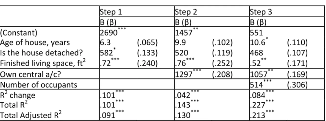
Table 5. Summary table for stepwise regression model of total electrical energy used in summer 2008 (kWh) vs. household characteristics.
N=284, ***p<=0.001;**p<=0.01; *p<=0.05.
Step 1 Step 2 Step 3
B (β) B (β) B (β) (Constant) 2690*** 1457** 551 Age of house, years 6.3 (.065) 9.9 (.102) 10.6* (.110) Is the house detached? 582* (.133) 520 (.119) 468 (.107) Finished living space, ft2 .72*** (.240) .76*** (.252) .52** (.171) Own central a/c? 1297*** (.208) 1057** (.169) Number of occupants 514*** (.306) R2 change .101*** .042*** .084*** Total R2 .101*** .143*** .227*** Total Adjusted R2 .091*** .130*** .213*** Next we examine the results of models for energy use during peak periods. We see patterns similar to those in the total energy use models (Tables 4‐5), but with some interesting nuances. The model for the summer peak time‐of‐use hours (Table 6) explains less variance than the model for all summer hours (Table 5), and ownership of central a/c actually declines in importance. However, in the model that includes only the top 1 % of summer systemwide demand hours (Table 7) ownership of central a/c supplants number of occupants as the most important predictor. Table 6. Summary table for stepwise regression model of total electrical energy used in peak period in summer 2008 (kWh) vs. household characteristics. N=284, ***p<=0.001;**p<=0.01; *p<=0.05.
Step 1 Step 2 Step 3
B (β) B (β) B (β) (Constant) 413*** 198 43 Age of house, years .6 (.033) 1.3 (.066) 1.4 (.072) Is the house detached? 117* (.136) 106* (.123) 97 (.113) Finished living space, ft2 .14*** (.239) .15*** (.250) .11** (.180) Own central a/c? 226** (.183) 185** (.150) Number of occupants 88*** (.266) R2 change .101*** .033** .064*** Total R2 .101*** .133*** .197*** Total Adjusted R2 .091*** .121*** .183***
11
Table 7. Summary table for stepwise regression model of total electrical energy used in top 1% of system use hours in summer 2008 (kWh) vs. household characteristics.
N=284, ***p<=0.001;**p<=0.01; *p<=0.05.
Step 1 Step 2 Step 3
B (β) B (β) B (β) (Constant) 64.0*** 24.9* 9.8 Age of house, years ‐.11 (‐.050) .00 (.002) .02 (.007) Is the house detached? 17.8** (.178) 15.8** (.158) 15.0* (.149) Finished living space, ft2 .013** (.184) .014** (.201) .010* (.142) Own central a/c? 41.2*** (.288) 37.1*** (.260) Number of occupants 8.6*** (.223) R2 change .096*** .080*** .045*** Total R2 .096*** .176*** .221*** Total Adjusted R2 .086*** .164*** .206*** Finally, we move to the regression models in which the correlation coefficient during the peak period is the outcome variable (Table 8). To reiterate, we calculated the simple correlation coefficient between a house’s hourly electricity use during the peak period, and the systemwide demand during the same period, this yielded one correlation coefficient per house per season. We then used household characteristics to predict these correlation coefficients. In this case, the only significant predictor of these correlation coefficients is the presence of central a/c. Although the variance explained by central a/c ownership is similar in this model to that in the model using the top 1% of system use hours (Table 7), the variance explained by all variables in our limited predictor set is substantially lower than in the energy use models (Tables 4‐7). It appears that while variables such as house size and number of occupants affect how much energy is used during peak periods in absolute terms, the shape of the daily use curve is not affected by these variables.
12
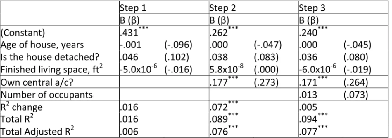
Table 8. Summary table for stepwise regression model of correlation coefficient between house and Ontario southwest region demand in peak period in summer 2008 vs. household characteristics.
N=284, ***p<=0.001;**p<=0.01; *p<=0.05.
Step 1 Step 2 Step 3
B (β) B (β) B (β) (Constant) .431*** .262*** .240*** Age of house, years ‐.001 (‐.096) .000 (‐.047) .000 (‐.045) Is the house detached? .046 (.102) .038 (.083) .036 (.080) Finished living space, ft2 ‐5.0x10‐6 (‐.016) 5.8x10‐8 (.000) ‐6.0x10‐6 (‐.019) Own central a/c? .177*** (.273) .171*** (.264) Number of occupants .013 (.073) R2 change .016 .072*** .005 Total R2 .016 .089*** .094*** Total Adjusted R2 .006 .076*** .077*** Discussion Our analysis indicates that the characteristics of houses that use more electricity on peak tend to be the same as those that use more electricity in total, although the on‐ peak analysis does refine the conclusions somewhat. The analysis of total annual electricity use suggests that higher usage is associated, as expected, with dwellings that have more occupants, more floor space, central a/c, and are older. By focussing on use during summer peak periods, the importance of central a/c ownership came to the fore. For energy use during the top 1% of system use hours, central a/c ownership was the strongest single predictor of household energy use, and was the only significant predictor when the outcome variable was the correlation coefficient between household energy use and Ontario southwest region demand in the summer peak period. This suggests that utilities similar to this one in southern Ontario desiring to reduce household electricity use at peak times in the summer should focus on reducing a/c load, above all other factors. There are voluntary programs that address a/c load already, such as Ontario’s Peaksaver [OPA, 2010], described above. These programs are typically advertized to all customers, but more focussed marketing is possible. If the utility has access to hourly data, they could simply focus on households with higher loads during peak hours. This does not necessarily identify houses with air conditioners, but hourly data should facilitate such identification, by examining which houses show large increases in usage on hot days. Targeting programs towards houses
13 with air conditioners and a high number of occupants may be even more cost‐effective, but data on number of occupants is difficult to obtain. If hourly data is not available, then house size and type are secondary factors for targeting households to improve uptake in peak reduction programs. Acquiring such data may be possible for some utilities with direct access to municipal property databases or by looking at the development date and characteristics of subdivisions. We had access to a relatively large sample of whole‐house hourly data, data that was typically unavailable to researchers in the past. However, our household characteristics data were limited compared to some prior studies. For example, although central air conditioning was a relatively strong predictor of summer electricity use on peak, the final model explained only around 20 % of variance, suggesting there are other important predictors not available to our models, and that exploring these other predictors would be essential to a fuller understanding of the determinants of household electricity use. An ideal future study would combine a large hourly energy use data set and new energy metrics with a detailed set of household characteristics and socio‐economic data for every house. The household characteristics and socio‐ economic data should include the variables used by Cramer et al. [1985]. This would allow for a model in which socio‐economic variables affect energy metrics indirectly through their effect on physical variables [Cramer et al., 1985], or a path analysis technique [Steemers & Yun, 2009], which should suppress the complicating effect of multicolinearity on the interpretation of results. Furthermore, our results were derived from data from a single municipality in southern Ontario. The effects of the various predictor variables might be quite different in a different location with a different climate, building practices, cultural attitude to energy use, and fuel mix. Future work should address a variety of locations. Conclusions Several prior studies have explored the effect of household characteristics on electrical energy use. This paper follows these analyses in a southern Ontario sample in 2008, and introduced two new ideas: • Availability of whole‐house hourly data from “smart” or “advanced” meters allows analyses that are restricted to peak periods only. Such analyses may become more widespread as hourly (and sub‐hourly) residential metering infrastructure is rolled out across North America. • As well as energy use in various periods, a new outcome metric was introduced: the correlation between an individual household’s hourly demand and that of the regional grid. Households with high values tend to
14 use more of their energy when overall grid demand is high; such households are of particular interest to utilities seeking to reduce peak demand. Results of the analyses confirm that larger houses with more occupants use more energy over all time frames, and reinforce the importance of air conditioning on peak use in summer. Such information can help utilities to better target demand‐side management programs, and refine future load growth forecasts. More information, and guidance for utilities, may have been garnered had we had a larger set of household characteristics, particularly household income and an appliance inventory. References Chong, H., 2010. Building vintage and electricity use: old homes use less electricity in hot weather. Energy Institute at Haas (EI @ Haas) Working Paper Series, WP211. URL: http://ei.haas.berkeley.edu/pdf/working_papers/WP211.pdf (last visited 2010‐12‐22) Cramer, J.C., Miller, N., Craig, P., Hackett, B.M., Dietz, T.M., Vine, E.L., Levine, M.D., Kowalczyk, D.J., 1985. Social and engineering determinants and their equity implications in residential electricity use. Energy, 10 (12), 1283‐1291. Granger, C.W.J., Kuan, C.‐M., Mattson, M., White, H., 1989. Trends in unit energy consumption: the performance of end‐use models. Energy, 14 (12), 943‐960. Hackett, B., Lutzenhiser, L., 1991. Social structures and economic conduct: interpreting variations in household energy consumption. Sociological Forum, 6 (3), 449‐470. Henley, A., Peirson, J., 1998. Residential energy demand and the interaction of price and temperature: British experimental evidence. Energy Economics, 20, 157‐171. Herter, K., Wayland, S., 2010. Residential response to critical‐peak pricing of electricity: California evidence. Energy, 35, 1561‐1567. IESO, 2010. Independent Electricity System Operator, Market Data. URL: http://www.ieso.com/imoweb/marketdata/marketData.asp (last visited 2010‐07‐19) Kaza, N., 2010. Understanding the spectrum of residential energy consumption: A quantile regression approach. Energy Policy, 38 (11), 6574‐6585. Kohler, D.F., Mitchell, B.M., 1984. Response to residential time‐of‐use electricity rates. Journal of Econometrics, 26, 141‐177. Navigant, 2008. Evaluation of Time‐of‐Use Pricing Pilot. Presented to Newmarket Hydro, and delivered to the Ontario Energy Board. URL:
15 http://www.oeb.gov.on.ca/OEB/Industry+Relations/OEB+Key+Initiatives/Regulated+Price+Plan/Regulat ed+Price+Plan+‐+Ontario+Smart+Price+Pilot Newsham, G.R., Bowker, B.G., 2010. The effect of utility time‐varying pricing and load control strategies on residential summer peak electricity use: a review. Energy Policy, 38 (7), 3289‐3296. Newsham, G.R., Birt, B.J., Rowlands, I.H., 2011. A comparison of four methods to evaluate the effect of a utility residential air‐conditioner load control program on peak electricity use. Energy Policy, 39 (10), 6376‐6389. OEB, 2010. Regulated Price Plan Price Report, May 1, 2010 to April 30, 2011. Ontario Energy Board. URL: http://www.oeb.gov.on.ca/OEB/_Documents/EB‐2004‐ 0205/RPP_PriceReport_20100415.pdf OPA, 2010. Ontario Power Authority. URL: http://everykilowattcounts.ca/residential/peaksaver/ Poulsen, M.F., Forrest, J., 1988. Correlates of energy use: domestic electricity consumption in Sydney. Environment and Planning A, 20, 327‐338. Pratt, R.G., Conner, C.C., Cooke, B.A., Richman, E.E., 1993. Metered end‐use consumption and load shapes from the ELCAP residential sample of existing homes in the Pacific Northwest. Energy and Buildings, 19, 179‐193. Rowlands, I.H., 2008. Demand Response in Ontario: Exploring the Issues. Prepared for the Independent Electricity System Operator (IESO). URL: http://www.ieso.ca/imoweb/pubs/marketreports/omo/2009/demand_response.pdf Steemers, K., Yun, G. Y., 2009. Household energy consumption: a study of the role of occupants. Building Research & Information, 37 (5‐6), 625‐637. Strapp, J., King, C., Talbott, S., 2007. Ontario Energy Board Smart Price Pilot Final Report. Prepared by IBM Global Business Services and eMeter Strategic Consulting for the Ontario Energy Board. URL: http://www.oeb.gov.on.ca/OEB/Industry+Relations/OEB+Key+Initiatives/Regulated+Price+Plan/Regulat ed+Price+Plan+‐+Ontario+Smart+Price+Pilot