Automated auscultation : using acoustic features to diagnose mitral valve prolapse

Automated Auscultation: Using Acoustic Features

to Diagnose Mitral Valve Prolapse

by

Marcia Yeojin Jung

S.D., Electrical Engineering and Computer Science

Massachusetts Institute of Technology (2003)

Submitted to the Department of Electrical Engineering and Computer

Science

in partial fulfillment of the requirements for the degree of

Master of Engineering in Electrical Engineering and Computer Science

at the

MASSACHUSETTS INSTITUTE OF TECHNOLOG

OF TECHNOLOGY

May 2004

2

0

2004

@Marcia

Y. Jung, MMIV. All rights reserved.

LIBRAR

3

The

publicly distribute paper and electronic copies of this thesis document

in whole or in part.

A uth or ...

Department of Electrical Engineering andCompu e Scihce

Ma. 20, 2004

C ertified by ...

Dorothy W. Curtis

Research Scientist, Computer Science & Artificial Intelligence

Laboratory

Thesis Supervisor

Accepted by ...

Arthur C. Smith

Chairman, Department Committee on Graduate Theses

Automated Auscultation: Using Acoustic Features to

Diagnose Mitral Valve Prolapse

by

Marcia Yeojin Jung

S.B., Electrical Engineering and Computer Science

Massachusetts Institute of Technology (2003)

Submitted to the Department of Electrical Engineering and Computer Science on May 20, 2004, in partial fulfillment of the

requirements for the degree of

Master of Engineering in Electrical Engineering and Computer Science

Abstract

During annual physical examinations, a primary-care physician listens to the heart using a stethoscope to assess the condition of the heart muscle and valves. This process, termed cardiac auscultation, is the primary means of diagnosing cardiac dis-orders, the most common of which is Mitral Valve Prolapse (MVP). Yet, the practice of auscultation is highly fallible with reports of more than 80% of MVP referrals to cardiologists being unnecessary.

The overall goal is to develop an inexpensive, easy-to-deploy software application to detect Mitral Valve Prolapse. Using an electronic stethoscope, audio and EKG data were simultaneously recorded for 51 subjects. The data was then manipulated and a prototypical beat, representative of an individual's pathology, was generated based on Z. Syed's work1.

This thesis presents a method for analyzing this prototypical beat. We extract 31 features from the prototypical beat, focusing on systolic activity. We then use the feature set as input to a radial-kernel support vector machine (SVM), which gives a binary classification of the subject as an MVP or non-MVP patient. We support our decision with a visual time-frequency decomposition of a patient's prototypical beat and relevant features.

Of the 51 subjects in our test set, we report three false negatives and five false

positives. We achieve 82% sensitivity while reducing the false-positive rate to 15%.

Thesis Supervisor: Dorothy W. Curtis

Title: Research Scientist, Computer Science & Artificial Intelligence Laboratory

'Zeeshan Syed (MIT '03) developed an algorithm to generate a prototypical beat as part of his M.Eng. thesis work.

Acknowledgments

My personal thanks to all the people that have been a part of this project. I am indebted to all the researchers and doctors who have contributed to this work, par-ticularly Dorothy Curtis, who provided indispensable guidance and inspiration. I am deeply grateful for the endless amounts of time and insight she so generously con-tributed. Also, my thanks to Professor John Guttag, Dr. Robert Levine and Dr.

Francesca Nesta for their efforts and support.

I would also like to thank my family and friends for their untiring support and encouragement, especially my parents who have been so understanding and selfless with me. To my friends, thanks for all the good wishes and caring.

Finally, I'd like to thank MIT for having given me such a tremendous opportunity.

My experience at MIT has been long and grueling, but also incredible. The things

I've learned and the relationships I've forged, I will carry with me for the rest of my life. Thank you.

Contents

1 Introduction

1.1 Problem Statement . . . .

2 Background

2.1 Review of Cardiac Functions . . . 2.1.1 Heart Physiology . . . . . 2.1.2 Cardiac Cycle . . . . 2.2 Mitral Valve Prolapse . . . .

2.3 Heart Murmurs . . . . 2.3.1 Murmurs caused by Mitral

3 Prototypical Beat Construction 3.1 Beat Segmentation . . . .

3.2 Time-Frequency Decomposition . 3.3 Median Filtering . . . . 3.4 Band Aggregation . . . .

Valve Prolapse

4 Prototypical Beat Analysis

4.1 Normal Cardiac Event Detection ...

4.2 Feature Selection ... ...

5 Classification

5.1 Support Vector Machines. . . . .

5.2 Data ... ... 13 14 17 17 17 18 20 21 22 25 25 26 27 28 29 29 32 39 39 40

5.3 Testing Methodology . . . .. . . .

6 Evaluation 43

6.1 Quantitative Performance . . . . 43

6.2 Qualitative Analysis . . . . 45

6.3 Performance Comparison to Previous System . . . . 48

6.4 Per Dimension Analysis . . . . 50

7 Related Work 53 7.1 Z. Syed and D. Curtis . . . . 53

7.2 W.R. Thompson et al. . . . . 54

7.3 C.G. DeGroff et al. . . . . 55

7.4 T.R. Reed et al. . . . . 56

7.5 I. El-Naqa et al. . . . . 57

8 Summary, Future Work and Conclusions 59 8.1 Future Work . . . . 59

8.2 Conclusions . . . . 60

A Detailed Results 61 A.1 Table of Results . . . . 61

A.2 False Negative Figures . . . . 61

B Supplementary Figures 67 B.1 Per-Dimension Plots of MVP and non-MVP Samples . . . . 67

List of Figures

2-1 Chambers and Valves of the Heart. . . . . 18

2-2 Typical EKG Waveform ... 19 3-1 Simultaneously Recorded Audio and EKG Signals. Courtesy of Z. Syed. 26

4-1 S1, S2, and Floor Value Demarcation in a Prototypical Beat . . . . . 32

4-2 S1, S2, and Floor Value Demarcation using 20% Default . . . . 33

4-3 S1, S2, and Floor Value Demarcation with High-frequency Content 33

4-4 Murmur Demarcation in Prototypical Beat of an MVP File . . . . 35

4-5 Murmur Demarcation in Prototypical Beat of a Normal File . . . . . 35 6-1 6-2 6-3 6-4 6-5 6-6 6-7 6-8

Example of False-Positive with a Benign Murmur False-Positive File C15SO . . . . Example of False-Negative File . . . . Example of Succinct MVP Murmur . . . . Example of Holo-systolic MVP Murmur . . . . Example of Quiet S1 Sound in MVP File . . . . . Example of Corrected False Positive . . . . Plot MVP vs. non-MVP Values for Murmur Dur Frequency Band . . . . . . . . 4 4 . . . . 4 5 . . . . 4 6 . . . . 4 7 . . . . 4 8 . . . . 4 9 . . . . 5 0 ation in 350-550 Hz

6-9 Plot of MVP vs. non-MVP Values for Slope of Murmur in 350-550 Hz

Frequency Band . . . . A-1 False-Negative I . . . . A-2 False-Negative II . . . . 52 52 64 65

B-1 Per-Dimension Plots (i)peakmag₂ (ii)peakmag₃ . . . . . . 67

B-2 Per-Dimension Plots (iii)peakmag₄ (iv)peakdur2 (v)peakdur3 (vi)peakdur4

(vii)peakslope2 (viii)peakslope3 . . . . 68

B-3 Per-Dimension Plots (ix)peakslope₄ (x)peakonset2 (xi)peakonset3 (xii)peakonset4

(xiii)peaktobandenergy2 (xiv)peaktoslenergy2 . . . . 69

B-4 Per-Dimension Plots (xv)peaktos2energy2 (xvi)peaktobandenergy3 (xvii)peaktoslenergy3

(xviii)peaktos2energy3 (xix)peaktobandenergy4 (xx)peaktoslenergy4 . 70

B-5 Per-Dimension Plots (xxi)peaktos2energy4 (xxii)sltobandenergy, (xxiii)s2tobandenergy1

(xxiv)sltobandenergy2 (xxv)s2tobandenergy2 (xxvi)sltobandenergy3 . 71

B-6 Per-Dimension Plots (xxvii)s2tobandenergy3 (xxviii)sltobandenergy4

List of Tables

6.1 Summary of Overall Results ... 45

A.1 Table of Results for Normal and Benign Subjects . . . . 62 A.2 Table of Results for MVP patients . . . . 63

Chapter 1

Introduction

During annual physical examinations, a primary-care physician listens to the heart using a stethoscope to assess the condition of the heart muscle and valves. This process, termed cardiac auscultation, is the primary means of diagnosing cardiac disorders, the most common of which is Mitral Valve Prolapse (MVP). Mitral Valve Prolapse is considered to affect up to 5% of the general population [10]. However, the practice of auscultation is highly fallible with a substantial number of unnecessary referrals to cardiologists. This is because detecting relevant symptoms and forming a diagnosis based on heart sounds is a skill that can take years to acquire and refine.

The human heart produces sounds having low frequency (20-1000 Hz), large dy-namic range and rapidly changing content. And, the human ear can often be fooled

by many of the subtleties of heart sounds. Part of the difficulty stems from the fact

that heart sounds are often separated from one another by less than 30 ms [17]. Com-pounding the matter, the energy in the most relevant part of the signal is often far less than (at times, less than a thousandth of) the total energy. The analysis of heart sounds consequently remains a challenge for many physicians.

Improved cardiac auscultation could have a significant impact on the quality and cost of medical care. The contemporary "gold standard" tests are expensive and often unnecessary. As many as 87% of patients referred to cardiologists have only benign heart murmurs [17]. The resultant inefficiency is substantial, as the cost of a visit to a cardiologist (including associated echocardiography) runs anywhere from $300

to $1000 in the United States [17]. In addition, there are also many forms of heart disease that remain asymptomatic and, therefore, undetected until they eventually deteriorate into serious medical disorders.

The goal of the auscultation section of the Patient Centric Network project at MIT's Computer Science and Artificial Intelligence Laboratory is the design, imple-mentation and evaluation of an inexpensive-to-deploy and easy-to-use software appli-cation system that can be used, in the office of a primary-care physician, to determine whether further examination, by means of an echocardiogram and consultations with cardiac specialists, is appropriate. The system aims to make a recommendation and support its decision with visual diagnostic aids, such as images of a prototypical heartbeat and relevant features. In addition, the system should present its recom-mendations in a transparent manner that can be validated in light of physiological knowledge. By doing so, the group hopes to demystify auscultation, and thereby improve the quality of its practice.

1.1

Problem Statement

The research presented here is part of an ongoing project of the aforementioned Patient Centric Network group. In particular, our work builds heavily upon the thesis work of Zeeshan Syed, who developed a preliminary system to detect Mitral Valve Prolapse through automated auscultation [22]. This project aims to extend and improve Syed's work in this area.

Several aspects of Syed's technical approach to the problem of automated aus-cultation are preserved in this work. Specifically, Syed's concept of a prototypical beat, generated from raw recordings of audio and EKG signals, as representative of a patient's pathology is fundamental to our work. This project seeks to gain a better understanding of the prototypical beat, and thereby fully leverage the information present in it. We do so by computing a feature set, characterizing different diagnostic features present in the prototypical beat. Using this feature set, we employ a support vector machine as a binary classifier in a new multi-dimensional feature space [11].

Finally, we extend Syed's library of visual aids, used to support the findings of the system, to include these new features in the display of the prototypical beat.

Chapter 2

Background

In this section, we offer a brief review of relevant cardiac terminology1 , followed by

a discussion of heart murmurs with particular emphasis on murmurs associated with Mitral Valve Prolapse.

2.1

Review of Cardiac Functions

2.1.1

Heart Physiology

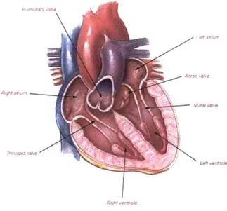
The heart consists of four chambers: the right and left atria and the right and left ventricles [4]. The two atria act as collecting reservoirs for blood returning to the heart while the two ventricles act as pumps to eject the blood to the body. De-oxygenated blood returns to the heart via the major veins (superior and inferior vena cava), enters the right atrium, passes into the right ventricle, and from there is ejected to the pulmonary artery on the way to the lungs. Oxygenated blood returning from the lungs enters the left atrium via the pulmonary vein, passes into the left ventricle, and is then ejected to the aorta.

In addition, the heart has four major valves, which ensure the unidirectional flow of blood throughout the system. The atria are separated from their respective ventricles

by the atrioventricular (AV) valves. More precisely, the tricuspid valve separates the

'This information comes from medical literature and is the widely aceepted view of cardiac

Ledtsmw~

@2002 Edwards Lifesciences Corp.

Figure 2-1: Chambers and Valves of the Heart

right atrium from the right ventricle while the mitral valve separates the left chambers of the heart. Two more valves, the semilunar (SL) valves, close off the ventricles from the arteries to which they lead. The pulmonary valve separates the right ventricle from the pulmonary artery and the aortic valve separates the left ventricle from the

aorta. Collectively, these four valves prevent the back-flow of blood in the heart.

2.1.2

Cardiac Cycle

The cardiac cycle refers to the sequence of events in the heart from the beginning of one heart-beat to the beginning of the next. Physiologically, an electrical impulse originates at the Sinoatrial node (SA node) and is conducted through the heart mus-cle, causing the atria to contract and then the ventricles, and, finally, causing the unidirectional flow of blood throughout the human body.

The cardiac cycle is comprised of two phases: systole and diastole. Systole is surrounded by two major heart sounds, commonly referred to as a "lub-dub" pair. The first heart sound (Si) corresponds to the shutting of the atrioventricular (AV) valves (i.e. mitral and tricuspid valves). The second heart sound (S2) indicates the

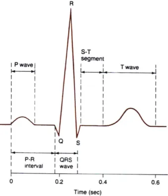
R S-T segment I Pwavej I I T wave S P-R i _{QRS I} nterval I wave I 0 0.2 0.4 0.6 Time (sec)

Figure 2-2: Typical EKG Waveform

closing of the aortic and pulmonary valves.

The electrical activity which causes the heart's chambers to contract can be recorded and expressed by an electrocardiogram (EKG). In analyzing the heart's electrical signal (EKG), the QRS complex reflects depolarization of the ventricular membrane, which directly causes ventricular contraction. The contraction of the ven-tricles then causes a rapid increase in intra-ventricular pressure, causing the AV valves to shut. As mentioned, closure of these valves results in the first heart sound (Si).

Furthermore, in the EKG signal, the T-wave indicates repolarization of the ventri-cles, causing them to relax. The timing of the T-wave in the cardiac cycle corresponds to a decrease in intra-ventricular pressure due to the outflow of blood. When the ven-tricular ejection rate reaches zero, the aortic and pulmonary valves shut, causing the second heart sound (S2). Thus, we conclude that S2 occurs in a small time window following the T-wave in the corresponding EKG signal.

It is important to note that both S1 and S2 correspond to the shutting of two separate pairs of valves. Thus, both S1 and S2 are not instantaneous events, but

rather they persist for some small duration of the cardiac cycle. The first heart sound with its mitral and tricuspid components, lasts for an average period of 100-200 ms, its frequency components lie in the range 10-200 Hz [8]. As for S2, the closure of the aortic valve and the pulmonary valve can often be separated by 20 ms and each component is approximately 10-30 ms in duration. The entire second heart sound contains frequencies in the range 10-400 Hz. The second heart sound usually has higher frequency content than the first heart sound because of the lesser mass of blood present in the cardiac chamber at the end of systole. The first and second heart sounds are separated by approximately 300-400 ms [8].

In our work, we define systole to be from the R-wave in the QRS complex, as found in the EKG signal, to the peak of the second heart sound (S2) in the audio signal.

2.2

Mitral Valve Prolapse

Mitral Valve Prolapse (MVP) is the most common condition affecting the valves of the heart [10]. The mitral valve is composed of two triangular flaps, which billow up to close off the channel between the chambers on the left side of the heart. Mitral Valve Prolapse refers to a malfunction where the two leaflets bulge (or prolapse) into the left atrium, preventing the mitral valve from closing properly. As a result, rather than a unidirectional flow of blood, some blood may leak back into the atrium. Mitral Valve Prolapse is thought to affect 2-5% of the adult population in the United States. In spite of its prevalence, many people with MVP never exhibit signs or symptoms of the condition. When symptoms do occur, they can vary widely. More common signs of MVP include an irregular heartbeat (arrhythmia), dizziness, difficulty breath-ing, fatigue and anxiety [5]. However, no unique set of physical symptoms exists to diagnosis Mitral Valve Prolapse. Most frequently, a primary-care physician detects MVP during a routine examination of the heart using a stethoscope, a procedure termed auscultation. If an individual suffers from MVP, abnormal heart sounds, including a characteristic clicking noise or murmur, will be often be present. To

con-firm the diagnosis, a specialist often conducts an echocardiogram. An echocardiogram uses high-frequency ultrasound waves to create a visual image of the heart, including the mitral valve and the flow of blood through it. By analyzing the sonar image, a cardiologist can, make a more definitive diagnosis. In some cases, further tests may be necessary, including chest X-rays, color Doppler ultrasound and/or cardiac catheterization. However, echocardiograms are widely considered the "gold-standard" in diagnosing MVP.

Complications associated with MVP are rare. Still in instances of severe regur-gitation, there is an increased risk of developing bacterial endocarditis, an infection affecting the mitral valve and/or the heart's lining. Consequently, many doctors pre-scribe prophylactic antibiotics to individuals with moderate to severe MVP. In more serious cases, surgery to repair or replace the faulty valve is recommended to pre-vent complications associated with further deterioration. Yet, for the vast majority of people with MVP, no special treatment is necessary and simple monitoring of the condition is sufficient [5].

2.3

Heart Murmurs

Heart murmurs are irregular sounds produced by the heart, often described as a swishing or whistling noise. Murmurs may be innocent or indicative of a more serious heart pathology. Benign murmurs, also called functional murmurs, are a result of turbulent blood flow, causing the walls of the heart to vibrate. Murmurs may also be caused by malfunction or malformations of the heart valves. Such a condition causes a regurgitation of blood (backwards across the valve), which accounts for the murmur.

Heart murmurs are characterized according to intensity (loudness), frequency (pitch), configuration (shape), quality, duration, direction of radiation, and timing in the cardiac cycle [2]. Establishing these features is the basis for drawing diagnostic conclusions about the murmur. Classification of murmurs is critical in distinguish-ing innocent murmurs from pathological murmurs, as well as identifydistinguish-ing the various

pathological conditions.

2.3.1

Murmurs caused by Mitral Valve Prolapse

Murmurs caused by Mitral Valve Prolapse have a unique acoustic signature. Follow-ing a normal S1 and a brief period of quiet, the valve suddenly prolapses, at times producing an audible, mid-systolic click. This click is sufficient to diagnose MVP, even without the presence of a subsequent murmur. Yet, often times, the click is succeeded by a crescendo-decrescendo murmur, which peaks at some point between mid to late systole [23]. Specifically, the murmur is a result of the turbulent backflow of blood across the prolapsed mitral valve. As the left ventricle contracts, pressure increases in the chamber. Eventually, the pressure forces blood back into the left atrium. The flow of blood through a small orifice, between the faulty flaps of the mi-tral valve, produces a high frequency murmur spanning 200-1000 Hz. In the case of significant mitral regurgitation, MVP may reveal a holosystolic murmur. The mitral valve, in such cases, is so compromised that it permits the backflow of blood over the entire systolic period, in contrast to the more typical late-systolic murmur.

The murmur is usually most audible at the apex of the heart, between the fifth and sixth intercostal spaces. This area is known as the mitral region of the anterior chest during auscultation and, as such, is particularly relevant to diagnosing MVP. In addition to the location at which to listen for the murmur, physical maneuvering of the patient is significant. Physical maneuvers may enhance the quality of the murmur. In particular, dynamic maneuvers, including Valsalva and prompt standing, decrease left ventricular volume. And in doing so, they cause earlier prolapse of the mitral valve and a longer associated murmur. Having the patient in supine position (i.e. lying on his/her back) produces similar results to the Valsalva maneuvers [2].

Other possible indicators of Mitral Valve Prolapse include a quiet S1 and a widely split S2 [15]. As previously noted, S1 corresponds to closure of the AV valves, with the mitral valve dominating. Since valve closure is faulty in individuals with MVP,

S1 may be noticeable quieter. Also in cases of severe regurgitation, the decreased

Recalling that S2 indicates shutting of the aortic and pulmonary valves, early closure of the aortic valve results in a widely split S2 sound.

This information related to the timing, frequency, and location of heart murmurs is the basis for our approach to diagnosing cardiac pathologies using acoustic signals.

Chapter 3

Prototypical Beat Construction

As discussed in Section 2.3.1, Mitral Valve Prolapse can be identified by examining the latter half of systole for abnormal cardiac activity. In order to make a diagnosis, the MAAS algorithm, developed by Zeeshan Syed, creates a prototypical beat [22].

A prototypical beat will lose some information related to the variations among beats

but has the benefit of suppressing some noise.

This section reviews the construction of a prototypical beat from the acoustic and EKG data. The progression from raw data to a prototypical beat can be seen in the following subsections. First, the audio signal is segmented into individual beats using the synchronously-recorded EKG signal. Next, a time-frequency decomposition is applied to the individual beats, separating each beat into 16 frequency bands. A prototypical beat is then constructed from the separate beats using median filtering. Finally, the 16 frequency bands of the prototypical beat are aggregated into 4 bands to be further analyzed.

3.1

Beat Segmentation

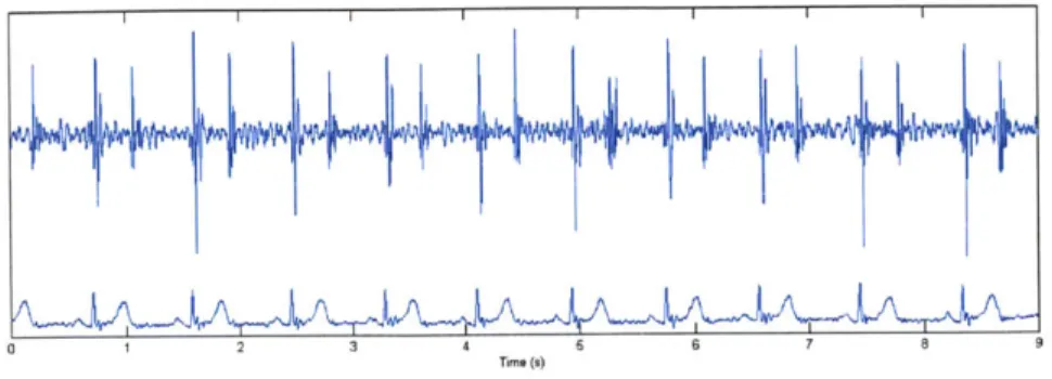
The recorded audio and EKG data are first processed to extract beats considered to contain the most diagnostic information [22]. The program begins by reading in the raw audio and EKG signals, sampled at rate of 44,100 Hz, and produces indexed vectors. The next task is to segment the audio signal into individual beats. This is

0 1 2 3 4 Tm s) 6 6 7 6 rie (8)

Figure 3-1: Simultaneously Recorded Audio and EKG Signals. Courtesy of Z. Syed.

done by using the synchronous EKG signal to find the indices associated with the onset of the QRS complex and the T-wave. The R-wave of the QRS complex indicates the onset of electrical activity associated with a given beat. These indices are used as preliminary reference points. Using a window about the T wave indices, a search is conducted to locate the peak of the S2 sound of each beat in the audio data. Thus, we have indices of the R-wave, T-wave and S2 peak for each beat.

Having segmented the audio signal into individual beats, the algorithm now selects beats for analysis based on a "Length-biased Admission of Noise-free Beats" criterion. That is, the program omits those beats considered to be too noisy for useful analysis while it is biased to admit beats of suitable length [22].

3.2

Time-Frequency Decomposition

As mentioned in Section 2.3.1, the acoustic signature of Mitral Valve Prolapse consists of energy at higher frequencies during the latter half of systole. Therefore, both the frequency composition and the timing of cardiac events are important in diagnosis, so a time-frequency decomposition is applied to the audio data.

To precisely analyze the frequencies in the selected beats, the program uses a filter bank that analyzes each heart-beat using a series of sharp frequency filters. As a special note, the filters must have narrow transition bands so minimal blurring of information occurs between adjacent frequency bands. This proves to be critical to the solution because the magnitude of lower frequency energy is often far greater than that of higher frequencies; so trends at higher frequencies will be masked otherwise [22].

In all, the filter bank consists of sixteen bans, each spanning a 50 Hz interval from 50 to 850 Hz. By opting to use such a filter bank, the algorithm maintains high fidelity to the timing of cardiac events while revealing trends at different frequencies. Now, a time-frequency analysis provides us with the frequency components in sixteen bands for each selected beat.

3.3

Median Filtering

In order to observe trends persisting amongst the majority of the beats, a mechanism to merge information from multiple beats to create a single representative heart-beat for the patient is developed. In other words, the program assimilates information from the selected beats to generate the time-frequency decomposition of a hypothetical "typical" beat for the patient. Such a time-frequency decomposition will be organized into the same sixteen frequency bands as mentioned in Section 3.1.

The prototypical beat is constructed as follows. The algorithm begins by taking the absolute value of the audio data and lining up selected beats in time for each of the sixteen frequency bands. Next, for each of the frequency bands, it finds the median four amplitudes of the beats at all time instances. The program then computes the means of the four median values at every time instance for each of the bands and makes them the associated values of the prototypical beat.

Although the construction of the prototypical heart-beat loses some variations between beats, it does not result in a significant loss of relevant information. Pa-tients suffering from Mitral Valve Prolapse exhibit pathological signs in the majority

of recorded beats. Therefore, the median values are believed to correspond to four beats, all possessing the MVP acoustic signature. In addition, noise may cause nor-mal patients to have one or more beats with energy at high frequencies, but it is improbable that the median four beats will include these outliers. And so, the pro-gram generates a time-frequency decomposition of a prototypical beat, representative of a patient's physiologic condition.

3.4

Band Aggregation

As a final step, the sixteen frequency bands are combined into four frequency bands, spanning 50-150 Hz, 150-350 Hz, 350-550 Hz, and 550-850 Hz. The bands are aggregated in such a way that energy at lower frequencies does not drown out higher frequency content, i.e. higher frequency bands are weighted more heavily [22]. Thus, we have a four-band frequency decomposition of a prototypical beat for a patient.

Chapter 4

Prototypical Beat Analysis

Previous work by Z. Syed describes the construction of a prototypical beat from audio and EKG data [22]. Syed's analysis of the prototypical beat is detailed in Section

7.1. This chapter outlines our analysis of the prototypical beat. First, we begin

with the topic of normal cardiac event detection and discuss the method of locating normal cardiac events in a prototypical beat. The following section elucidates the feature selection process, which generates a feature set to be used later in the decision mechanism.

4.1

Normal Cardiac Event Detection

After constructing a prototypical beat for a given patient, our program must identify the following normal cardiac events as reference points: R-wave position, peak of S1 position, beginning of S1, end of S1, peak of S2 position, beginning of S2 and end of

S2 sound. These events are calculated in the baseband and serve as reference times in

the higher frequency bands. We also calculate a floor value for each frequency band of the prototypical beat.

Let Zi be the one-dimensional array containing the time-frequency content of a prototypical beat in the i-th frequency band. Specifically, Z1, Z2, Z3 and Z4 correspond

to content in the 50-150 Hz, 150-350 Hz, 350-550 Hz, and 550-850 Hz frequency bands, respectively.

As described in Section 3.3, the prototypical beat was constructed by lining up the selected beats in time. Specifically, the R-wave in the EKG signal associated with each beat was indexed at 4410 samples. We consider this point, i.e. the peak R-wave of the QRS complex, as the proposed onset of systole in our prototypical beat. We label this point q.

Next, the peak of the S1 sound is chosen by searching, in the baseband, for the position of the maximum amplitude in a window 100 ms before to 150 ms after the onset of the QRS complex. That is,

slpeakpos = maxpos [Z 1(q - 100 ms : q + 150 ms)]

and s1peakamp is the associated amplitude.

Now, designating the position of the S2 peak requires some backtracking. From the original audio signal, we calculate the median S2 peak position of the selected beats. We call this value m. After doing so, we search a 1600 sample window centered at this median value. So,

s2peakpos = maxpos [Zl(m - 800: m + 800)]

and, similarly, s2peakamp is the corresponding amplitude.

At this point, the floor value for each band is computed. We do so by, first, dividing systole (as defined in Section 2.1.2) into ten equal intervals and, then, averaging the points in each interval.

systoliclength = s2peakpos - q

intervaLavgij = avg [Zi(q + j * systolic ength : q + (j + 1) * systolidength

The floor value is determined as the minimum of the ten averages.

floorvali = min [intervaLavgi,o , interval-avgi,1 , ... , intervaLavgj,9]

The next defined reference point is the end of the S1 sound. This is designated as the first point to the right of the S1 peak where the baseband component hits the band's floor value.

slend = minpos [Zl(slpeakpos : slpeakpos + systolidength) < floorvali]

If no such point exists within the first third of systole, the program, by default, marks the farthest right point, in the same window, where the data is below 20% of the peak Si amplitude as the end of S1.

slend = maxpos [Zl(slpeakpos : s1peakpos + 3?J'*o'icienfth) < 0.2 s1peakamp]

In contrast, the beginning of the S1 sound is defined to be concurrent with the R-wave of the associated EKG signal. This is because, physiologically, we know that the onset of the QRS complex precedes S1 by an instant, as mentioned in Section 2.1.2. Furthermore, we have previously defined this point for the prototypical beat and labeled it "q".

Finally, the S2 sound must be isolated in a similar fashion. The first points to the left and right of the S2 peak where the data hits the floor value mark the bounds of S2. And if no left bound is found within a window of one third of systole before the peak

S2 sound or if no such bound exists to the right, then the bounds are established at

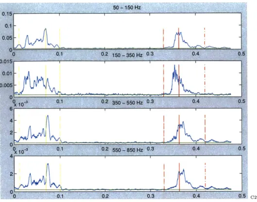
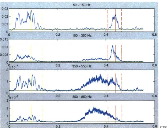
20% of peak S2 magnitude. These points are labeled s2begin and s2end, respectively.1 Figure 4-1 illustrates the above result of detecting normal cardiac events. The solid yellow line indicates the peak of the S1 sound in the baseband (slpeakpos). The dotted yellow lines mark the bounds of the S1 sound. Likewise, the solid red line represents the peak of the S2 sound, with the dotted red lines marking the edges. The horizontal green line represents the floor value for each band. Notice that the dotted lines representing slend, s2begin, and s2end are found to be at the points where the signal hits the floor value in the base band. By contrast, Figure 4-2 shows an example where the signal does not hit the floor within the first third of systole and, therefore, the default 20% is used to mark the end of S1. Also, the figures show that the demarcation of S1 and S2, as found in the baseband, is directly extended to the higher frequency bands. The significance of doing so is apparent in Figure 4-3, which corresponds to an MVP patient. By using the baseband to determine the

'Later modifications to the system look for a dip in S2 in the baseband and redefines the beginning

U U. I U: U. a I WV-4 C29S1

Figure 4-1: S1, S2, and Floor Value Demarcation in a Prototypical Beat

bounds of S2, it is evident that much of the high frequency content visible in bands 2,3, and 4 is not due to harmonics associated with the S2 sound but rather mitral regurgitation.

4.2

Feature Selection

Having defined the above reference points, our program now generates a feature set, characterizing systolic activity in a prototypical beat. Specifically, the pro-gram calculates the following features: peakmagk, peakonsetk, peakdurk, peakslopek, peaktobandenergyk, peaktoslenergyk, peaktos2energyk, sltobandenergyi, s2tobandenergyi, s1width and s2width; where i E {1,2,3,4}, k e {2,3,4}. The following section defines these features and details the derivation of each. In order to make valid comparisons between patient files, the calculation of many features includes a normalization step. As discussed in Section 2.3.1, the acoustic signature of Mitral Valve Prolapse consists of energy at higher frequencies during the second half of systole. Therefore,

-50 - 150 Hz

0.1 0.2 350 -550 Hz 0.3 0.4 0.5

0.1 02 5 0. 0.4 0.5

0.1 0.2 0.3 0.4 0.5 C37SO

Figure 4-2: Si, S2, and Floor Value Demarcation using 20% Default

50 -150 Hz

0 0 123S1

we begin by searching for a peak between the midpoint of systole to the beginning of

S2 in each of the three higher frequency bands. The position of this peak is defined

as follows,

peakposk = maxpos [Zk(q + sy*2tiden : s2begin)]

2

and the related amplitude is called peakampk.2

The first feature, peakmagk, describes the magnitude of the mid-systolic peak with respect to the floor value of that band. Specifically,

k = peakampyk

peakmagk _foorvalk

We hypothesize that the mid-systolic peak is the crest of the murmur caused by MVP. Consequently, we proceed to search for the beginning and end of the murmur. We define the bounds to be the first points to the left and right of the peak where the signal is below 25% of the peak magnitude. If the signal does not go below the

25% level, the end of Si and the beginning of S2 are set as the default ends of the

murmur.3

peakbegink = maxpos [Zk(slend : peakposk) < 0.25 peakampk] peakendk = minpos [Zk(peakposk : s2begin) < 0.25 peakampk]

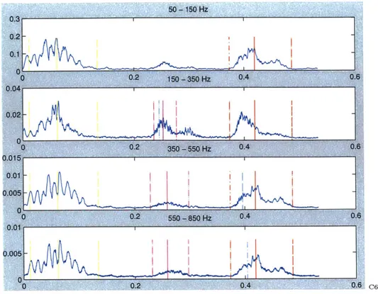
Figures 4-4 and 4-5 illustrate how the program searches for a late-systolic peak, as indicated by the solid magenta line, in each of the three higher frequency bands. The dotted magenta lines mark the bounds associated with this peak, while the horizontal cyan line represents the 25% threshold used to determine the bounds. In addition, the figures demonstrate the differing results produced by the program when processed over files corresponding to a physiologically normal subject versus an MVP sufferer.

The feature, peakonsetk, determines the onset of the proposed murmur in the cardiac cycle.

2If _{the position of the peak is found to be concurrent with the beginning of S2, the program backs}

off 10 ms and re-searches for a peak in systole. 3

If the 25% value is less than the band's floor value, then the floor value is used to mark the ends

50 - 150 Hz 0.3 0.2-0.1 0 0 0.2 150 - 350 Hz 0.4 0.6 0.04 0.02'-A 0 0 0.2 350 - 5%, Hz 0.4 0.6 0.015 0.01 - 0.005-0 0.2 550 - 850 Hz 0.4 0.6 0.01 0.005 0.6 C65SO

Figure 4-4: Murmur Demarcation in Prototypical Beat of an MVP File

50 -150 Hz

C29SO

Figure 4-5: Murmur Demarcation in Prototypical Beat of a Normal File

... , .. . .

0.4

peakonsetk = _{systolidength}peakcegink

In addition, two other features, peakdurk and peakslopek, are calculated using the bounds of the murmur. The former quantifies the duration of the murmur with respect to systolic length. The second estimates the ascending slope of the murmur, using the peak point and the point found as the start of the murmur. As mentioned in Section 2.3.1, murmurs associated with MVP exhibit specific morphologies. And

so, we attempt to quantify the shape of the murmur using the feature, peakslopek.

peakdurk = peakendk-peakbegink systoliclength

peakslopek = peakampk-Z k(peakbegink)

peakposk-peakbegink

Next, our program computes the energy of the murmur with respect to three dif-ferent cardiac events. First, the energy of the murmur is calculated as a fraction of the total energy in the related frequency band. We call this feature peaktobandenergyk. Second, the murmur's energy is found with respect to the energy associated with S1 in each band (peaktoslenergyk). Finally, the energy of the murmur is derived as a fraction of the energy of S2 (peaktos2energyk).

peaktobandenergyk = sum[Zk(peakbegink:peakendk) Sum[Zk]

eakt gy= sum[Zk(peakbegink:peakendk)]

peaftosenergYk = msum[Zk(slbegin:slend)

g

= sumZA(peakbegink:peakendk)]

peaktos2energYk = sum[Zk(s2begin:s2end)]

Having collected a set of features describing systolic activity, our program proceeds to compute statistics about other cardiac events. Now including the baseband (Z1),

the energy associated with the S1 sound in each band is calculated as a fraction of the total energy in the frequency band. The bounds of S1 remain constant across the frequency bands and are given by the beginning and end times of S1 found in the baseband. This feature is labeled sltobandenergyi. Similarly, the relative energy associated with S2 is calculated for each band (s2tobandenergyi).

sltobandenergyj _soanenegy1 = sum[Zi(s1begin:slend)]_{sum[Zi ]}

Lastly, two final features, slwidth and s2width, describe the duration of the S1 and S2 sounds with respect to systolic length.

slwidth = slend-slbegin

systoliclength

s2width = s2end-s2begin

Chapter 5

Classification

After compiling a feature set describing a patient's cardiac activity, our final step is to make a diagnosis based on the information. Specifically, we use an off-the-shelf, radial kernel Support Vector Machine as a binary classifier [11]. We start with a brief overview of support vector machines, followed by a discussion of our dataset and our testing methodology.

5.1

Support Vector Machines

The support vector method is a recently developed technique designed for efficient multi-dimensional function approximation [3]. The basic idea of support vector ma-chines (SVMs) is to determine a classifier that minimizes the empirical risk, i.e. the training set error, and the confidence interval (corresponding to the generalization, or test set, error). Effectively, the method tries to find a hyperplane that separates the multi-dimensional data perfectly into two classes.

In SVMs, the idea is to fix the empirical risk associated with a kernel's architec-ture and, then, to use a method to minimize the generalization error. The primary advantage of SVMs as adaptive models for binary classification is that they provide a classifier with minimal Vapnik-Chervonenkis (VC) dimension, which implies low expected probability of generalization errors [3].

issues. First, an appropriate architecture, or model type, must be selected according to the sample space. Otherwise, even with zero empirical risk, it is possible to have a large generalization error. Next, to avoid over-fitting, it is necessary to minimize the VC dimension of the model when training on large, high-dimensional datasets. However, in doing so, we sacrifice some margin of empirical risk. A final concern is determining the parameters of our learning algorithm. Such parameters include generalization and kernel parameters.

SVMs can be used to classify linearly separable data and nonlinearly separable data, depending on the kernel function. The kernel function refers to the formula used to calculate an inner-product in some feature space. A radial basis function automatically determines centers, weights and thresholds that minimize an upper-bound on the expected generalization error, drawing non-linear upper-boundaries in the multi-dimensional feature space [3].

After experimenting with our dataset, we determine that our problem is well-suited to using a radial-kernel support vector machine as a binary classifier, where each of the features calculated in Section 4.2 are used to create a multi-dimensional feature space.

5.2

Data

This work is made possible through the efforts of our collaborators at Massachusetts General Hospital. In particular, Dr. Francesca Nesta collected data, using an elec-tronic stethoscope, from patients referred for echocardiograms. In addition, data was gathered from families with one or more members diagnosed with MVP. The data collected from the latter group was recorded on-site, in the homes of the subjects. This is significant to understanding the poor quality-control environment in which the data was collected.

More specifically, our dataset consists of simultaneously-recorded audio and EKG signals for fifty-one patients. Of these patients, seventeen suffer from Mitral Valve Prolapse, and the remaining thirty-four have normal heart sounds or benign murmurs.

For each patient, multiple recordings were taken at different sites on the body, in different positions. In general, we find the audio signal taken from the apical region of the heart with the patient lying down on his/her left side to contain the most diagnostic information, as confirmed by Dr. Nesta. Other recorded sites and positions

include the second intercostal space with the patient sitting, squatting and lying on his/her left side.

Finally, in evaluating the performance of our system, it is important to note two other aspects of our dataset. First, many of our non-MVP test subjects were originally referred for an echocardiogram by their primary care physicians. That is, an early diagnosis flagged them as potentially having MVP. The significance of this is that a correct negative classification of any of these files is an improvement on the performance by the primary-care physicians. Another important point to consider in evaluating our system is that all files were labeled according to the re-sults of an echocardiogram examination. Echocardiograms are widely considered the gold-standard for diagnosing MVP. Therefore, we trust these labels and compare our system's results in relation to them.

All data was sampled at 44.1 kHz with 16-bit quantization. Each data file is

approximately 30 seconds long. In addition, all data is de-identified with files assigned labels of the form CxxSxx (where xeK).

5.3

Testing Methodology

To test the performance of our system, we use a leave-one-out cross-validation scheme. For each patient, we train the SVM on the other 50 patients' files to create a test model. The model is then used as the basis for classifying the given patient. Therefore, we generate 51 different test models, one corresponding to each patient.

As mentioned, our dataset consists of 51 patients with multiple files for each. Through experimentation with each MVP patient's data, we decide upon a "best" file, which corresponds to the file with the most diagnostic information. For physiologically normal patients or those with benign murmurs, we include all files associated with

the patient. We choose this selection of files as our test set to ensure that every MVP sample point contains physiological evidence of MVP and, therefore, representative features of the condition. In order for the SVM to create an accurate model from its training set, each sample point must be indicative of its corresponding classification. Therefore, we include only a single file per MVP patient while admitting all files of a non-MVP patient.

We then proceed to classify each patient, on a per-patient basis using his/her file set, as suffering from MVP or not. More precisely, after the SVM conducts a binary classification of each file associated with a patient, our program aggregates the results of the patient's files and positively classifies the patient if any of his/her files were considered to exhibit MVP characteristics. Therefore, we justify including a solitary file per MVP patient because only one of the patient's files needs to be positively classified to correctly classify the patient. In contrast, correct classification of non-MVP subjects requires accurate classification of all the corresponding files.

Finally, through experimentation, parameters for the SVM are optimized to ob-tain the best results. In general, we find the SVM to be surprisingly insensitive to parameter changes. Specifically, we examined different values of the parameter C and gamma. The parameter C controls the trade-off between training error and margin, where lower values signify greater tolerance of training error and, therefore, better generalization [12]. Establishing an upper bound on C prevents over-fitting of the model. The parameter gamma relates to the radial-basis kernel function. Testing values of C from 1 to 1000 and values of gamma from 0.1 to 2, results show minimal variation in performance over a wide range of parameter settings. Best results were achieved with values of C from 10-1000 and gamma from 0.8-1.8. We select C=1000 and gamma= 1.0 as a representative configuration of the SVM classifier for the rest of this study.

Chapter 6

Evaluation

This chapter presents the results obtained by our system. We begin with a quantita-tive assessment of the detector's performance on a per-patient basis. This is followed

by a qualitative analysis of our program, as revealed by the visual feature set and the

SVM models that were generated. Also, in this chapter, we compare the performance of our classification system to Syed's system.

6.1

Quantitative Performance

As discussed in Section 5.3, we conducted leave-one-out cross-validation tests for

51 patients. Of the 51 patients, we incorrectly classified eight patients, three false

negatives and five false positives. A false negative corresponds to the misclassification of an MVP patient. On the other hand, a false positive signifies that at least one of the files associated with a normal (or benign) subject is incorrectly classified. And

so, the patient is falsely flagged as an MVP candidate.

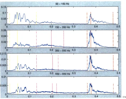
Our false positive rate of approximately 15% is a significant improvement from the previously quoted 87% found in some primary-care settings. Of the five false positives we obtained, we found that four of the patients suffer from benign murmurs with trace or mild regurgitation. And the prototypical beats of these patients show a non-trivial systolic murmur such as that seen in Figure 6-1. We consider these patients to be acceptable false positives as they exhibit significant, abnormal cardiac

50 - 150 Hz 0.15 01 0 2 10 - 350 Hz 0. A 0.51 0.05 -0f0 0.1 0.2 150 -850 Hz 0.3 0-4 0.5 0.01- 0.040-0. 0.2' 6 -5~ 0.3 0.4 0.5 3 1

Figure 6-1: Example of False-Positive with a Benign Murmur

activity and merit further examination of their condition. Also, we believe that with more samples of early-systolic benign murmurs such as that found in Figure 6-1, the SVM will be better able to distinguish between MVP and benign murmurs.

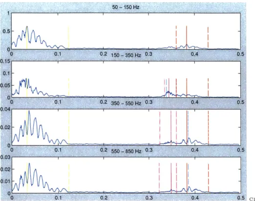
Our remaining false positive corresponds to the file in Figure 6-2. This file (and therefore patient) is incorrectly classified because harmonics associated with S2 at higher frequencies are left-shifted, occurring prior to the dominant harmonics of S2 in the baseband. Consequently, our system considers the high-frequency energy as part of an MVP murmur. We consider this an anomalous case.

Of more serious consequence, our system fails to correctly classify three cases of MVP. In these cases, the telling murmur occurs so closely to S2 that our system fails to distinguish it from the second heart sound. This could be a reflection of real physiological circumstances, where MVP murmurs of brief duration occur

just

50 - 150 Hz 0 ~ 0.1 0.2 150 - 350 Hz 0.3 0A 0.5 0.15 01 I 0.05 0 . 0230 5 H 30. :

Figure 6-2: False-Positive File C15SO

Also, refer to Tables A.1 and A.2 in Appendix A for individual results obtained per patient.

Sensitivity Specificity False Negative False Positive Overall Results: 82% 85% 1 3 5

Table 6.1: Summary of Overall Results

6.2

Qualitative Analysis

In Syed's work, classification was based on the timing of the murmur in the three frequency bands spanning 150-350 Hz, 350-550 Hz, and 550-850 Hz. As discussed in Section 2.3.1, murmurs associated with Mitral Valve Prolapse have a unique acoustic signature with many well-documented characteristics. In order to make more thor-ough use of this medical information, we generate a fuller feature set to better capture

w 0 0.1 0.2 5W - 850 Hz 0.3 0.4 0. 0.03 0.020.01 -0 0.1 0.2 0.3 0.4 0. 5 5 C1SO

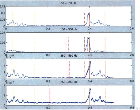
50 - 1 SOH~z 0.1 0 -0 ~ 0.2 150 - 350 Hz 0.4 0.6 0.04 0.02-0. 4--2 0 00 0.4 0;6 C73S11

50 - 150 Hz 0.3 0.2OA -0 _{0.2 0.4 0.6} 150 - 350 Hz 0.04 0 0.2 3W "5W KZ OA 0.015, 0.01 0.005 0 0 0.9 550 - 850 Hz o.4 .0.6 n ni 6 C65S0

Figure 6-4: Example of Succinct MVP Murmur

the qualities of the murmur. This section discusses the performance of our system in characterizing cardiac activity associated with Mitral Valve Prolapse.

Among our system's contributions, our work measures the intensity of the mur-mur by calculating its associated energy. In doing so, we better equate MVP-related murmurs of varying morphology. For example, loud, click-type murmurs and rela-tively quiet, persistent murmurs report comparable energy measurements, and both are indicative of MVP. Compare, for instance, the energy of the murmur found in Figure 6-4 to that found in Figure 6-5.

Now, expanding on Syed's description of timing, we calculate features designating the onset, peak and duration of the murmur. This is particularly relevant to charac-terizing holo-systolic murmurs such as that found in Figure 6-5. Here, it is evident that our system is capable of capturing the entire murmur.

Finally, we include features to gauge the energy and duration of the S1 and S2 sounds, as medical information suggests that Mitral Valve Prolapse may cause an unusually quiet S1 and/or a widely split S2 sound. Figure 6-6 demonstrates one

U U.Z U.4 U.0 C68S1

Figure 6-5: Example of Holo-systolic MVP Murmur

such case of MVP where the S1 sound is uncommonly muted in comparison to other cardiac activity.

6.3

Performance Comparison to Previous System

In the figures found in this chapter, the dashed, vertical cyan lines indicate the points that are used by Syed's system to classify the same file.' While the difference in quan-titative performance is marginal, closer examination of the results reveals important differences between the two systems. The following section details these differences.

First, Syed's approach is better able to handle cases where MVP murmurs occur very close to the second heart sound. In the false-negative example shown in Figure

6-3, Syed's program captures part of the narrow murmur occurring just prior to S2

and correctly classifies the file.

Yet, in Figure 6-4, consider the dashed cyan lines in the 350-550 Hz and 550-850

Figure 6-6: Example of Quiet S1 Sound in MVP File

Hz frequency bands. In these bands, Syed's system misses the evident murmur by simply using the points, demarcated by the cyan lines, to classify the file. Fortunately, Syed's system catches the murmur in the 150-350 Hz frequency band and ultimately classifies the file correctly. However, this case demonstrates the potential loss of information that Syed's approach risks.

Also, in Figure 6-6, it is possible that Syed's system correctly classifies the file for the wrong reason. That is, Syed's system misses the low amplitude, persistent, late-systolic murmur and classifies the file based on the location of the dashed cyan lines. This point may indeed be part of a sharp murmur immediately preceding

S2. However, Syed's program may instead be catching part of an S2 harmonic and

considering it an MVP murmur. More importantly, Syed's program fails to identify the more apparent MVP murmur in the file. This suggests that Syed's system is using the wrong feature to correctly classify the file while our system more accurately delimits the murmur as shown by the dashed magenta lines.

.uC35S4

Figure 6-7: Example of Corrected False Positive

consider variability in duration of S2 among subjects. As detailed in Section 7.1, classification is based on a comparison in timing of the maximum amplitude of the baseband in the latter half of systole and the location of the dashed cyan lines.

By only considering a single point of S2, Syed's program is prone to flagging early

harmonics associated with S2 as MVP murmurs, and therefore misclassifies some normal patients. In contrast, our system first demarcates the bounds of S2 in the baseband and then proceeds to search for a peak outside of that range in the upper frequency bands. Figure 6-7 illustrates one such example where our system correctly classifies the normal patient but Syed's reports a false positive.

6.4

Per Dimension Analysis

Although each of our features is based on physiological knowledge of MVP murmurs, we found some features to be more critical and formative to the classification process. Employing an SVM approach to classification enables us to use a high-dimension

-feature space, yet we lose some transparency as a consequence. In order to gain a better understanding of the decision mechanism, we produce plots of sample points along each dimension. A radial-kernel SVM undoubtedly combines these dimensions and formulates decision boundaries in a complex manner, but our hypothesis is that certain dimensions show distinct clustering of negative and positive sample points, suggesting that the corresponding feature is a strong indicator of Mitral Valve Pro-lapse.

Figure 6-8 plots the values obtained for the feature corresponding to the duration of the murmur in the 350-550 Hz frequency band. The red points represent MVP patients and the green points represent non-MVP patients. As can be seen, the graph suggests that murmurs of duration less than 5% of systolic length indicate normal or benign conditions. Conversely, murmurs of longer duration are a strong indicator of Mitral Valve Prolapse. However, it is important to note that this feature, alone, is an imperfect indicator as there are non-MVP points occurring above the 0.05 value and MVP points present below. Nonetheless, the graph exhibits fairly strong clustering of MVP and non-MVP sample points along this dimension.

By contrast, Figure 6-9 shows a similar plot for the feature describing the slope of

the murmur found in the 350-550 Hz frequency band. Along this dimension, values of MVP and non-MVP files do not show any real separation. Such a plot suggests that the feature is not a strong indicator of MVP and is, therefore, not as germane to classification as the other features.

Refer to Appendix B.1 for equivalent plots of remaining features. While defini-tive statements on the significance of specific features are not possible, a qualitadefini-tive analysis of the plots lends some insight into the matter. Verification of findings is conceivable by omitting irrelevant features and evaluating the performance of new SVM models.

0.6 5 10 15 20 Patients Figure 6-8: Plot MVP vs. Frequency Band 5

non-MVP Values for Murmur Duration in 350-550 Hz

Band3 Peak Slope (8)

0.25 0.2 0.15 0.1 0.05 0 -0.05 0 10 15 20 25 Patients

Figure 6-9: Plot of MVP vs. non-MVP Values for Slope of Murmur in 350-550 Hz Frequency Band

Band3 Peak Duration (5)

MVP NOT MVP ---x---- -0.5 0.4 0.3 0.2 0.1 0 0 25 MVP -+-NOT MVP --- x----X. - *'Cx-..s~ 'x

Chapter 7

Related Work

7.1

Z. Syed and D. Curtis

As previously mentioned, Zeeshan Syed created an automated auscultation system to detect Mitral Valve Prolapse [22]. In that system, Syed first builds a prototypical beat and then, based on this "average beat", he uses a decision mechanism to classify patients based on band-specific time thresholds. For a given beat, in each of the three higher frequency bands (i.e. 150-350, 350-550, 550-850 Hz), the program searches for the earliest maximal point in the latter half of systole. The time of this position is then normalized by dividing by the beat's systolic length. Next, if this point occurs sufficiently prior to time of S2 in the base band (i.e., 50-150 Hz), then it is concluded that this peak in energy is due to MVP and not S2. If any of the three bands passes this criterion, then the beat and the patient are classified as having MVP.

In subsequent related work, Dorothy Curtis analyzed some potential algorithm re-finements. This work looked at several time-based threshold conditions. The leftmost time in the latter half of systole of 60%, 70%, 80%, and 100% of the maximum am-plitude in each of the three upper bands was considered. The time of this maximum was compared to the time of S2 in the baseband and to the time of the maximum amplitude in the baseband. (The point of maximum amplitude in the latter half of systole in the baseband was not necessarily co-incident with S2 in the baseband.) The best combination found compared the time of the earliest occurrence of 60% of the