IdEP Econom ic Papers
2015 / 05
O. Giuntella, F. Mazzonna
If you don’t snooze you lose health and gain weight : evidence
from a regression discontinuity design
If You Don’t Snooze You Lose Health and Gain Weight
Evidence from a Regression Discontinuity Design
Osea Giuntella∗
University of Oxford
Fabrizio Mazzonna†
Universit´a della Svizzera Italiana (USI)
First Draft‡
July 9, 2015
Abstract
Sleep deprivation is increasingly recognized as a public health challenge. While several studies provided evidence of important associations between sleep deprivation and health outcomes, it is less clear whether sleep deprivation is a cause or a marker of poor health. This paper studies the causal effects of sleep on health status and obesity exploiting the rela-tionship between sunset light and circadian rhythms and using time-zone boundaries as an exogenous source of variation in sleep duration and quality. Using data from the American Time Use Survey, we show that individuals living in counties on the eastern side of a time zone boundary go to bed later and sleep less than individuals on the opposite side of the time zone boundary. These findings are driven by individuals whose biological schedules and time use are constrained by social schedules (i.e., work schedules, school starting times). Exploit-ing these discontinuities, we find evidence that sleep deprivation increases the likelihood of reporting poor health status and the incidence of obesity. Our results suggest that the increase in obesity is explained by both changes in eating behavior and a decrease in physical activity. Keywords: Health, Obesity, Sleep Deprivation, Time Use, Regression Discontinuity
JEL Classification: I12; J22; C31
∗University of Oxford, Blavatnik School of Government and Nuffield College. 1 New Road, OX11NF, Oxford,
Oxfordshire, UK. Email: osea.giuntella@nuffield.ox.ac.uk.
†Universit´a della Svizzera Italiana (USI). Department of Economics, via Buffi 13, CH-6904, Lugano. Email:
fab-rizio.mazzonna@usi.ch. We are thankful to John Cawley, Martin Gaynor, Kevin Lang, Climent Quintana-Domeque, Daniele Paserman, and Judit Vall-Castello for their comments and suggestions. We are also grateful to participants at workshops and seminars at the University of Warwick, the University of Oxford, and Universitat Pompeu Fabra.
1
Introduction
Sleep is increasingly recognized as a fundamental public health challenge. Insufficient sleep is associated with higher incidence of chronic diseases (i.e. hypertension, diabetes), cancer, de-pression and early mortality (see Cappuccio et al., 2010, for a systematic review). Moreover, sleep duration may be an important regulator of body weight and metabolism (Taheri et al.,
2004;Markwald et al.,2013). In particular, medical literature associates sleep deprivation with a reduction of leptin level, the so-called “satiety hormone”, and with an increase of ghrelin level, also known as the “hunger hormon” (Ulukavak et al.,2004).
Through its effects on health capital and cognitive skills, sleep deprivation can have important effects on human capital and productivity (Hamermesh et al., 2008; Gibson and Shrader, 2014). Insufficient sleep has been also linked to motor vehicle crashes. For instance drowsy driving is responsible for 900 fatalities and 40,000 nonfatal injuries annually in the US (National Highway Traffic Safety Administration 2012). Yet, some estimates suggest that in many countries individ-uals are sleeping as much as two hours less sleep a night than people used to sleep a hundred years ago (Roenneberg,2013).
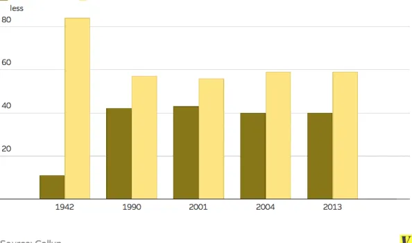
Figure 1illustrates the dramatic shift in the share of individuals reporting less than 6 hours sleep between 1942 and 1990. A survey conducted in 2013 by the U.S. National Sleep Foundation found that Americans are more sleep-starved than their peers abroad. The Institute of Medicine (2006) estimates that 50-70 million US adults have sleep or wakefulness disorder (Altevogt et al.,
2006). Using data from National Health Interview Survey, the Centers for Disease Controls and Prevention (CDC) shows that 37% of adults reported an average of less than 7 hours of sleep per day in 2005-2007. In 2009, only 31% of high school students reported getting at least 8 hours of sleep on an average school night. In light of these trends, a recent article on Nature,Roenneberg
(2013) argues that unnatural sleeping and waking times could be the most prevalent high-risk behavior in modern society and proposes a global human sleep study to restructure work and school schedules in ways that may better suit our biological needs.
Despite the increased attention of media and policy makers, the health and economic con-sequences of insufficient sleep are not yet well-understood. In particular, it is unclear whether sleep duration is a cause or a marker of poor health (Cappuccio et al., 2010). The goal of this paper is to analyze the causal effects of sleep deprivation on health.
The causal evidence on the effects of sleeping time has been so far limited to laboratory studies. As noted byRoenneberg(2013), laboratory studies offer a very limited understanding of both the determinants and consequences of sleep deprivation, as they are usually based on people who have been instructed to follow certain sleep patterns (e.g., bedtime), and are not sleeping on their beds, and are affected by laboratory settings (e.g., individuals are often required to sleep with electrodes fastened to their heads etc.). If sleep deprivation has causal effects on health, the sleep deprivation epidemic may have substantial costs for the health care systems.
The main contribution of this paper is to provide a causal estimate of the effects of sleep deprivation on health using time-use data that are more likely to capture real world sleeping
habits. In particular, we focus on the effects of insufficient sleep on general health status and obesity, one of the adverse health outcome associated with sleep deprivation.
There are several biological channels through which sleep deprivation may increase obesity. As mentioned above, medical research has shown that sleep deprivation reduces levels of leptin, a hormone made by adipose cells that regulates energy balance by inhibiting hunger; and ghrelin, a hunger-stimulating hormone, which regulates appetite and has the opposite effect of leptin, increasing hunger by stimulating gastric acid secretion and gastrointestinal motility in order to prepare the body for food intake (Ulukavak et al., 2004). Finally, behavioral studies show that sleep loss increases the likelihood of gaining excessive weight by increasing the consumption of fats and carbohydrates and reducing the likelihood of being engaged in moderate or intense physical activity (Greer et al.,2013;Markwald et al.,2013).
To identify the effect of sleep deprivation, we exploit the variation in sleeping induced by discontinuities in sunset time. More specifically, we exploit the fact that, at the time zone border, there is a sharp discontinuity in sunset time that affects the sleeping behavior of people living on the two sides of the time zone border. There is large medical evidence that shows how solar cues affect sleep timing (seeRoenneberg et al.,2007, for a review). The daily light-dark cycle governs the so-called circadian rhythms, rhythmic changes in the behavior and the physiology of most species, including men (e.g.,Vitaterna et al.,2001).
Studies have found that these circadian rhythms follow an approximately 24-hour cycle and are governed by the suprachiasmatic nucleus (SCN), or internal pacemaker also known as the body master’s clock. The SCN synchronizes biological rhythms to the environmental light, a processed knows as “entrainment”. When there is less light the SCN stimulates the production of melatonin, also known as ”the hormone of darkness”, which in turn promotes sleep in diurnal animals including humans (Aschoff et al.,1971;Duffy and Wright,2005;Roenneberg et al.,2007;
Roenneberg and Merrow, 2007). Therefore, we expect individuals living in areas where sunset occurs at a later time will tend to go bed later than individuals living in areas where sunset occurs earlier. In addition, as shown by Hamermesh et al. (2008), TV programs may affect bedtime because television schedules are typically posted in Eastern and Pacific time (see also Section1.1). Note that if people would compensate by waking up later this would have no effect on sleeping time. However, because of economic incentives and coordination social schedules, such as work schedules and school start times are usually less flexible than biological timing. Thus, many individuals will not be able to fully compensate in the morning by waking up at a later time.
Using sleeping data public available on the website of one of the US leader fitness tracker company1, Figure2 illustrates the clear discontinuity in bedtime at each time zone border. The bottom figure provides a zoom at the north border between the Eastern and the Central time zone. The figure shows that people living in counties on the eastern side of a time zone border go to sleep later than people in neighboring counties on the western side of the time zone boundary.
These differences in bedtime give rise to differences in sleep duration across time zone borders since many people cannot fully compensate. We show that this is particularly true for workers, because standard office hours are the same across borders, and for parents with children, because they have to bring them to school early in the morning.
There are other papers in the economic literature that exploit the variation in sunset time or in Daylight Saving Time (DST).Barnes and Wagner(2009) show that the transition into DST has only short-term effects on sleep. Doleac and Sanders(2013) use the discontinuous nature of DST and find large drops in cases of reported murder and rape. In a recent study Jin and Ziebarth
(2015) study the health effects of DST and find that health slightly improves in the short-run (4 days) when clocks are set back by one hour in the fall, but no evidence of detrimental effects when moving from standard time to DST in the Spring. Using a different approach and exploiting the time and geographical variation in sunset time within each time zone,Gibson and Shrader(2014) find that one-hour increase in average daily sleep raises productivity by more than a one-year increase in education. However, none of these papers exploit the sharp discontinuity at the time zone borders or analyze the medium and long-run health consequences of sleep deprivation.
Using data from the American Time Use Survey, we show that employed people leaving in counties bordering on the eastern side a time zone sleep on average 19 minutes less than em-ployed people living in neighboring counties on the opposite side of the border because of the one-hour difference in sunset time. Such difference in sleep duration gives rise to large differ-ences in obesity and self-reported health across borders. In particular, people on the eastern side of a time zone have 6 percentage points higher probability of being obese and are 3 percent-age points more likely to report a poor health status. It is worth noting that, especially in the case of obesity, these are the consequences of a long-term-exposure to sleep deprivation. This is confirmed by the evidence of larger effects among the older workers (over 40).
We then turn to the analysis of the possible mechanisms behind the relationship between sleep deprivation, health, and obesity. We find evidence that individuals on the eastern side of the time-zone border are more likely to eat late in the evening than their neighbors on the western side of the time-zone border—regardless of the number of times or the time spent eating earlier in the day. They are also more likely to eat out and less likely to engage in physically intensive activities. These results are consistent with some of the recent behavioral evidence on sleep deprivation and weight gain (Markwald et al., 2013) who note as sleep deprivation may induce fatigued individuals to eat more- in particular to eat more carbohydrates- to sustain their wakefulness while at the same time their exhaustion may reduce their physical activity leading to an increase in weight gain.
Finally, we show that there is no discontinuity in predetermined characteristics known not to be affected by the treatment (sleeping). In particular, that individuals’ height does not differ systematically across the time zone border and that there is no evidence of any significant rela-tionship with human capital indicators at the beginning of the 20th century when the time zones had not yet introduced in the United States.
People spend approximately one-third of their time sleeping, but there is remarkable varia-tion in sleeping. Variavaria-tion in sleeping may respond to economic incentives since higher wages raise the opportunity cost of sleep time (Biddle and Hamermesh,1990). Furthermore, sleep de-privation may affect directly human capital (cognitive skills) and productivity . Thus, shedding light on the determinants and consequences of sleep deprivation in a real-world setting is crucial to understand how working schedules, school start times, and TV schedules may be restructured to improve individual health and well-being, as well as productivity.
The remainder of this paper is organized as follows. In the remainder of this section we briefly discuss the background of the US time zones. Section 2 describes the empirical strategy along with the main identification issues. Section 3 presents the data used for our analysis and Section 4 presents some summary statistics presents our results. We discuss the mechanisms underlying our main results in Section 5. Section 6 illustrates a battery of robustness checks. Concluding remarks are in Section 7.
1.1 US Time Zones
As shown in Figure 3, continental United States are divided into 4 four main time zones (Eastern, Central, Mountain, and Pacific). The time zones were first introduced in US in 1883 to regulate railroad traffic. However, work scheduling was still not coordinated. Therefore, even areas in close proximity use to operate on different times (Hamermesh et al.,2008). The current four U.S. time zones were officially established with the Standard Time Act of 1918, and since then there have been only minor changes were operated at their boundaries. The Eastern time zone was set -5 hours with respect to the Greenwich Mean Time (GMT), and the other three time zones (Central, Mountain and Pacific) differ from that by -1, -2, and -3 hours respectively. It is worth noting that time zone borders do not always coincide with state borders since several US states (13) are follow different time zones.
The introduction of Daylight saving time (DST) was, instead, more troublesome. DST plan was also adopted in 1918, as an effort to save energy during the war, but it was soon repealed after the end of World War I because of its unpopularity. The current DST plan was introduced in 1966 in the Uniform Time Act and further changes to the DST schedule were made in 1976 and in 2007. US states are able to supersede the law. In particular, Arizona has never observed DST since 1967, while Indiana has only started to follow DST in 2006, with the exception of some counties at the border between the Central and the Eastern time-zone.
As shown byHamermesh et al. (2008), television programs importantly affect bedtime and, more generally, individual time-use. Television networks usually broadcast two separate feeds, namely the “eastern feed” that is aired at the same time in the Eastern and Central Time Zones, and the “western feed” for the Pacific Time Zone. In the Mountain Time Zone, networks may broadcast a third feed on a one-hour delay from the Eastern Time Zone. Television schedules are typically posted in Eastern/Pacific time, and, thus, programs are conventionally advertised as ”tonight at 9:00/8:00 Central and Mountain”. Therefore, in the two middle time zones television
programs start nominally a hour earlier than in the Eastern and Pacific time zones.
2
Empirical strategy
The empirical analysis of this paper focuses on the effect of sleep deprivation on health (obe-sity and self-reported health). A simple comparison of people with different sleeping behavior does not allow to identify the causal effect of sleep deprivation on health because of both reverse causality and several potential confounding factors (e.g. stress, occupation etc.).
In this paper, we address the identification problem by using a spatial regression discontinuity (SRD) design that contrasts the sleeping behavior of residents on either side of the three main US time zone borders (Eastern–Central, Central–Mountain and Mountain–Pacific).
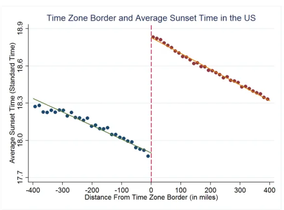
The intuition is that individuals in counties bordering on the eastern side of the time zone border go to bed later than people in neighboring counties on the opposite side of the border, because of the one-hour difference in sunset time. Yet, these individuals are otherwise similar. Figure 3 shows the sharp discontinuity in sunset time at the border aggregating the average sunset time of the US counties based on the distance (in miles) from the closest time zone border. This discontinuity is mirrored by the observed difference in average bedtime at the time-zone border (see Figure 2). We show that this difference in average bedtime generates significant differences in sleeping behavior as people on the eastern border of a time-zone boundary do not completely compensate for it by waking up later. This is especially true for workers that have to deal with standard office hours that are approximately the same across borders (office hours usually start at 8am or 9am) and for people with children in school age.
Our identification strategy exploits this spatial discontinuity in sleeping time. If we focus on a reasonable small bandwidth around each time zone and if we expect a causal relationship between sleep duration and health, the observed sleeping difference should generate differences in health (here measured using obesity and self-reported health) that should not be confounded by other observable and unobservable characteristics. For simplicity, we assume that the relation-ship between sleep duration and health is linear. Under this assumption, our estimation strategy allows us to estimate the effect of sleeping duration on health.
It is worth noting that the health differences across bordering counties, in particular in the case of obesity, are likely to be the result of a long-term exposure to “sleep deprivation”. In other words, what we measure when analyzing the effect of a hour increase in sleeping time is not the effect of one-hour difference in sleeping in night preceding the survey interview, but rather the average effect of a long-term exposure to one-hour difference in sleeping that depends on the time spent in a given location. Indeed, we show that this effect is larger for older people than for younger as older people have been exposed for a longer time period than younger people to differential sunset time. Moreover, if people often change their residence, it is likely that the estimated effect on health represents only a lower bound of the true effect, unless healthier individuals systematically move from the eastern to the western side of each time zone border.
From an econometric perspective, the general idea in a RD design is that the probability of receiving a treatment (an additional hour of sleep) is a discontinuous function of a continuous treatment determining variable (sunset time). However, the treatment in our case does not change from 0 to 1 at the time zone border. Our running variable, D, is the distance (in miles) from the time zone border. Distance is positive for counties on the eastern side of the border (D > 0) and negative for counties on the western side (D < 0). Let Ee(H) ≡ lime→0E(H|D = 0+e)
and Ew(H) ≡ lime→0E(H|D = 0−e) define the two sides expectation of our observed health
outcomes when approaching the border from East (e) and West (w).
If we assume that there are no other unobservable characteristics that change at the border, contrasting the health outcome H at the time zone border, Ee(H) −Ew(H), measures the effect
of the sleeping differences at the border generated by the time zone change. This identification is clearly fuzzy since it does not generate a sharp discontinuity in sleeping hours. In effect, people may partially offset the effect of the different sunset time by adjusting their sleeping or waking time. This means that we need to use a 2SLS strategy that “inflates” the reduced-form effect, Ee(H) −Ew(H), taking into account the sleep duration (S) difference at the border,
Ee(S) −Ew(S). Therefore, our fuzzy SRD design may be seen as a Wald estimator around the
time zone discontinuity:
τSRD =
Ee(H) −Ew(H)
Ee(S) −Ew(S)
.
2.1 Estimation
Specifically, we exploit the geographical variation in sunset time at the border estimating the following two equation:
Hic=α0+α1Sic+α2Dc+α3Dc∗EBc+Xic0 α4+Cc0α5+Iic0 α6+uic (1)
Sic=γ0+γ1EBc+γ2Dc+γ3Dc∗EBc+Xic0 γ4+C0cγ5+Iic0 γ6+νic (2)
where Sicis the sleep duration of the individual i in county c; EBc is an indicator for the county
being on the eastern side of a time zone boundary; Dcis the distance to the time-zone boundary
“running variable” (or forcing variable) using the county centroid as an individual’s location; the vector Xiccontains standard socio-demographic characteristics such as age, sex, education,
mar-ried and number of children; Cc are county characteristics, such as region (northeast, midwest,
south, west), latitude and longitude and whether the respondent live in a very large county.2 We also account for interview characteristics that might affect individual’s sleeping behavior (Iic),
such as interview month and year, a dummy that controls for the application of DST in county c, and two dummies that control whether the interview was during a public holiday or over the weekend. We control for the running variable using a local linear regression approach with a varied slope on either side of the cutoff.
2We control for the fact that for very large county the distance based on centroid might be a very noisy
Substituting the treatment equation into the outcome equation yields the reduced form equa-tion:
Yics =β0+β1EBc+β2Dc+β3Dc∗EBc+Xic0 β4+C0cβ5+Iic0 β6+eics, (3)
where β1 = α1∗γ1. Therefore we can estimate the parameter of interest α1 as the ratio of the
reduced form coefficients β1/γ1 via 2SLS. Standard errors are robust and clustered according to
the distance from each time zone border (10 miles groups).
As mentioned above, the main assumption behind our identification strategy is that the ob-served differences in health at the time zone border only reflect differences in sleeping behavior generated by the different sunset time. The underlying idea is that individuals in nearby coun-ties are similar along other characteristics. As any identification assumption this is directly untestable. However, using both individual and county level data, Table1illustrates that a large set of observable characteristics is well balanced in a relatively small bandwidth from the time zone boundary (within 250 miles). In Section4, we show that the effect the different sunset time at the border on sleep duration is robust to the inclusion of state fixed effects and to the restriction of our analysis to a very narrow bandwidth around the time zones (100 miles). Furthermore, in Section6we test for whether there are discontinuities in pre-determined characteristics for which we have data, but which are known not to have been affected by the treatment, and we find no evidence of significant differences across the border.
Finally, it is worth noting that the heterogeneity of our findings by employment status and family composition is consistent with our hypothesis that employed people and parents with children are less likely to fully adjust their sleeping behavior as a response to the different sunset time on the two sides of the border (see the result in Section4).
3
Data and descriptive statistics
In this paper we use data from the American Time Use Survey (ATUS) conducted by the U.S. Bureau of Labor Statistics (BLS) since 2003. The ATUS sample is drawn from the exiting sample of the Current Population Survey (CPS) participants. The respondents are asked to fill out a detailed time use diary of their previous day that also include information on time spent sleeping and eating. On average, more than 1,100 individuals participated to the survey each month since 2003 and the last available survey year is 2013. This yields a total sample of approximately 148’000 individuals. Our analysis restricts the attention to individuals in the labor force (both employed and unemployed)3 living within 250 miles from each time zone boundary (Pacific-Mountain, Mountain-Central, Central-Eastern). This is done by merging the ATUS individuals to CPS data to obtain information on the county of residence of ATUS respondents. Unfortunately, CPS does not release county information for individuals living in counties with less than 100,000 residents, thus we can match only 44% of the sample. We further restrict our sample to people age 18 to 55
3We exclude people not in the labor force because this category includes disable individuals due to an illness
to avoid the confounding effect of retirement and the selection issue that might arise focusing on young workers in high-school age. We also limit the analysis to individuals who sleep between 2 hours and 16 hours per night. After imposing these restrictions, the sample comprises 18,639 individuals of which 16,557 were employed. Employment status was determined on the basis of answers to a series of questions relating to their activities during the preceding week.
The variable of main interest is sleep duration. We count only the night sleeping by excluding naps (sleep starting and finishing between 7am and 7pm).4 We also consider alternative measure of sleeping time such as sleep at least 8 hours (or less than 6), bedtime and waking up time.
We evaluate the effect of sleep duration on obesity (BMI> 30) and the likelihood of report-ing a poor health status, defined as reportreport-ing poor or fair health status as commonly done in the literature using metrics of self-reported health status. Unfortunately, such important health information are not present in all survey years. In particular, questions on self-reported health status are only available since 2006, while information on body weight is available in the Eating Module included in the survey in the 2006-2009 waves.
In our analysis, we include several socio-demographic controls, namely age, sex, education, race, marital status and number of children that might affect individuals’ sleeping behavior. Moreover, we use geographic controls, such as census region and latitude, to avoid that other geographical factors might confound our analysis at the time-zone border.
In Table 1 we report summary statistics for the variables of interest for each side of the border. We focus on employed population.5 Specifically, Column 1 and 2 reports summary statistics for individual living, respectively, on the western (early sunset) and at the eastern (late sunset) side of one of the three main time zone borders. By construction, there is a large and significant difference in average sunset time between respondents living on the two sides of the time zone border. This difference seems to affects individual sleeping behavior. In particular, the table shows that early sunset respondents have significantly higher sleep duration. They sleep on average 10 minutes more and have a 4% higher probability to sleep at least 8 hours. This difference arises from the fact that they go to sleep later, but they do not compensate by waking up later (compare awake at midnight and awake at 7.30 am). On the contrary, the other individual characteristics are well balanced across the two groups. The only significant coefficient among the covariates is proportion of black people (see Column 3). However, as we account for the latitude this difference disappears as the higher presence of Blacks on the eastern side mostly reflects the high-density of African-Americans in the Eastern time zone in the South.
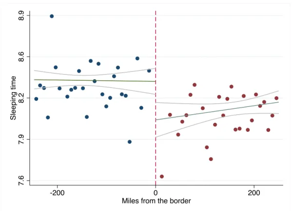
Figure4confirms the presence of a large discontinuity in sleep duration at the time zone bor-der for employed respondents of approximately 20 minutes. In particular, each point represents the sample mean of sleep duration for a group of counties aggregated according to the distance to the border.6 For purely descriptive purposes, the fitted lines are based on a linear fit within
4However, results are unchanged if including naps in the main variable (see Table13).
5However, there is no significant difference in the likelihood of being employed between individuals living on
opposite sides of the time-zone (coef., -0.010; std. err., 0.013.)
250 miles east and west of the border.
4
Main Results
4.1 First-Stage: Sleeping Time and Time Zones’ Borders
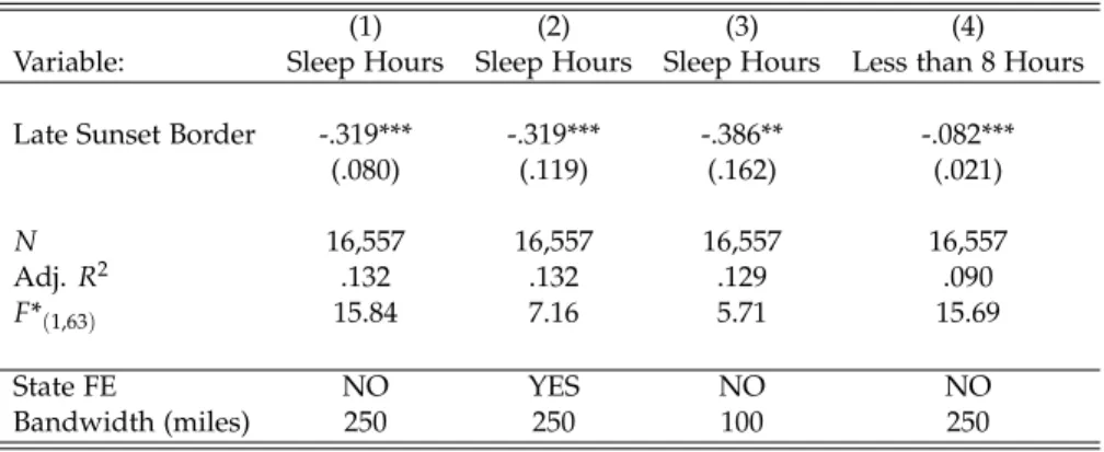
Table 2 illustrates the estimated effect of the being on the eastern border on sleep duration as in equation (2). In Column 1, we show that our baseline estimates coincide with the uncon-ditional evidence reported in Figure 4. After controlling for a large set of socio-demographic, geographical and interview characteristics, the estimated effect of being on the east border (“late sunset border”) is of approximately 19 minutes, reducing sleeping time by 0.2 standard devia-tions (see Table1). The other three columns confirm the robustness of our findings to the inclu-sion of additional controls, the use of different bandwidths and alternative metrics of sleeping. As thirteen US states are on two different time zones, in column 2 we can re-estimate the first-stage including a full set of state fixed effects (Column 2). Notably, the point estimates remain substantially unchanged. In column 3, we restrict the attention on a very narrow bandwidth of 100 miles (column 3). As the discontinuity in sunset time is larger at the border and diminishes with the distance for the border, it is not surprising to find even a larger effect on sleeping time. The coefficient indicates that within 100 miles from the border, individual on the eastern side of the border sleep on average 23 minutes less than their neighbors on the western side. Finally column 4 shows that there is a large effect also on the probability of sleeping less than 8 hours. Being on the eastern side of the boundary decreases the likelihood of sleeping at least 8 hours by 8.2 percentage points, which is equivalent to approximately 25% of the mean of the dependent variable in the sample.
In Table 3 we compare employed and non-employed respondents. Consistent with our hy-pothesis on working schedules’ constraints on sleeping time, the first two columns show that the late sunset time on the east border affects only the employed respondents. Columns 3-6 explain where the difference between employed and non-employed respondents comes from. In partic-ular, in columns 3 and 4, we show that regardless of their employment status individual on the eastern side of the time zone border are always more likely to go to bed later. The estimates show that being on the eastern side increases the likelihood of being awake at midnight by 12 percentage points for both the employed and the non-employed, a 60% increase with respect to the mean of the dependent variable. However, employed respondents are less likely to adjust their waking time accordingly. Column 5 shows no significant difference across the border in the likelihood of being awake at 7.30am for employed people. On the contrary, non-employed on the eastern side of the time zone border do adjust their waking up time in the morning. Col-umn 6 shows that non-employed individuals on the eastern side of the time zone border are 13 percentage points less likely to be awake at 7.30am, a 20% effect with respect to the mean of the dependent variable.
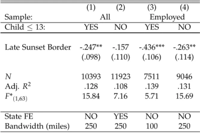
Similarly we would expect to find larger effects for individuals with children in schooling age, particularly families with young children who are not yet able to go to school on their own. As already mentioned, the idea is that parents who have to bring their young children to school early in the morning have less flexibility in the waking up time and, those living on the eastern side of the border, may therefore not be able to fully compensate for a later bedtime. Consistent with our hypothesis, Table 4 shows that the estimated effect is larger for people with children younger than 13. Columns 1 and 2 show that when analyzing the entire sample (employed and non-employed) the effect is larger and significant for individuals with children under the age of 13. Focusing on the employed population, column 3 shows that among individuals with children those living on the eastern side of the time zone border sleep on average 26 minutes less, while the point estimate is substantially lower among individuals without young children (column 4).
The fact that the heterogeneity of the results presented in Tables 3 and4 confirm our main hypotheses is reassuring and suggests that we are not confounding the effect of the late sunset with that of other confounding factors.
4.2 Effects of Sleeping on Health Status and Obesity
We exploit the discontinuity in sleeping time to evaluate the effects of sleeping time on obesity and self-reported health status. Again, we focus on the employed population, as we have shown that there is no significant discontinuity in sleeping time among the non-employed. As already mentioned, in the ATUS health information are not present in all survey years, thus, we have limited identification power. Despite that, the results in Table5show a significant effect of both health outcomes. In particular, Column 1 and 2 show the reduced-form and the 2SLS estimates on obesity, while Column 3 and 4 on poor health. Column 1 shows that employed individuals living on the eastern side of the time zone border are 6 percentage points more likely to be obese, approximately 22% with respect to the mean of the dependent variable in the sample under analysis. With regard to self-reported health status, column 3 shows that employed individuals on the effect is of almost 3-percentage points, almost 30% of the sample mean.
The IV estimates are obviously larger because of the fuzzy design of our RD strategy. As already mentioned, these estimates must be interpreted with caution. In effect, these health differences, especially in the case of obesity, are likely to be the result of a long-term exposure to sleep differences (caused by the different sunset time) on the two sides of the time zone border. Therefore, in the case of the IV estimates, the point estimates measures the causal effect of long-term exposure to “sleep deprivation” of one-hour. In the case of obesity the estimated effect is of almost 15-percentage points (58% of the mean) while for poor health of 8-percentage points (87% of the mean).
Increasing sleeping time by 19 minutes7, the average difference in sleeping time observed
7Note that the first-stage is larger in the sample for which we have information on BMI and health status indicating
an average difference in sleeping time at the border of 27 and 23 minutes respectively. However, the standard errors are relatively large and, thus, the firs-stage is not statistically different from the one reported in Table2showing that
at the time-zone border in the whole sample, increases obesity by approximately 4 percentage points, a 16% effect with respect to the mean of the dependent variable, and increases the like-lihood of reporting poor health status by 2.4 percentage points, a 26% effect with respect to the mean of the dependent variable.
Table 5 illustrates the heterogeneity of our result by age group. Consistent with our prior, columns 1 and 2 show the reduced-form effect on obesity is concentrated among older workers (column 2), who have been exposed to the treatment for longer than younger workers (column 1). On the contrary, the age gradient is small and not statistically significant when examining health status (columns 3 and 4). These differences are not surprising as self-reported health status is more likely to capture the short-term effects of sleep deprivation on health perception. In other words, self-reported health status is more likely to reflect idiosyncratic variations in sleeping time, while obesity is more likely to reflect the cumulative effect of sleep deprivation over time.
5
Mechanisms
The medical literature offers clear biological explanations for the effects of sleep deprivation on obesity. As mentioned above, medical research as shown that insufficient sleep affects the function regulating appetite and expenditure of energy. Previous studies provided evidence that food intake during insufficient sleep is a physiological adaptation to provide energy needed to sustain additional wakefulness and that sleep duration plays a key role in energy metabolism (Markwald et al., 2013) favoring the consumption of fats and carbohydrates. Furthermore, the fatigue due to sleep loss may reduce physical activity exacerbating the effects of sleep deprivation on weight gain. In this section, we examine how individuals’ time use and activities may respond to these biological mechanisms and affect caloric intake and expenditure.
Eating Habits
Insufficient sleep may increase calorie intake, particularly at evening as individuals start feel-ing tired and feel the need of energy to keep themselves awake. Markwald et al.(2013) present evidence of how changes in circadian rhythms may contribute to the altered eating patterns during insufficient sleep. In particular, they argue that a delay in melatonin onset, altering the beginning of the biological night, may lead to a circadian drive for more food intake at night. To verify whether this channel may contribute to explain our findings we examine individuals eating patterns on the two sides of the time zone border. Table 7documents that individual on the eastern side of a time-zone border tend are more likely than their neighbors on the opposite side of the border to eat after a given hour. In particular, they are 30% more likely to start a meal after 6pm, 46% more likely to start a meal after 7pm, and 50% more likely to start a meal after 8pm. These results hold accounting for the number of meals one has had before 6pm, 7pm, and individuals on the the eastern side of the border sleep approximately 19 minutes less than their neighbors living in counties on the opposite side.
8pm respectively, suggesting that people are not just shifting eating time to a later hour, but they are more likely to be eating after a given hour regardless of the number of times they ate earlier on.
Another possible explanation for the effects of sleep deprivation on obesity is that if individ-uals sleeping less are more tired in the evening, they may also be less willing to eat-out and more willing to eat outside. Indeed, previous studies show that because restaurants routinely serve food with more calories than people need, dining out represents a risk factor for overweight and obesity (Cohen and Story, 2014). To test this hypothesis, in Table8 we use information on the location of each activity reported in the ATUS time diary and construct indicators for whether individuals consumed their meal at home or out.
Column 1 shows that individuals on the eastern side of the time-zone boundary are 4 percent-age points more likely to eat-out. The coefficient stable once we control for the overall number of meals (column 2). However, the estimates are imprecise. Note also that column 1 and 2 include lunch-meals at the work-place. In column 3 and 4 we focus on the likelihood of having dinner out, measured as dining out after 5pm. Individuals on the eastern-side of the time zone border are 8 percentage points more likely to eat out after 5pm. On the contrary, we find no significant differences among non-employed individuals at the borders for both the likelihood of having late meals after a certain hours and the likelihood of dining out.8 Again, the results hold if we control for the number of meals one had before 5 pm or the overall time spent eating. Together, these findings suggest that insufficient sleep may affect obesity through its effects on the likelihood of having more meals/snacks after a given hour as well as the likelihood of eating out. The fact that results are robust to the inclusion of controls for previous number of meals/average time spent in previous meals suggests these differences in eating behaviors may lead to a net increase in caloric intake.
Physical Activity
Another potential explanation for the effect of sleeping on obesity is that insufficient sleep may reduce calorie expenditure because tired individuals are less likely to engage in physical activities. Using ATUS data on time spent walking, biking, or doing any kind of sport activity we do not find any evidence of significant differences between individuals on opposite sides of time-zone borders. However, we find some evidence that individuals on the eastern side of the time zone border are less likely to engage in activities of moderate, vigorous, or very vigorous intensity using metabolic equivalents associated to each activity reported in the ATUS time di-ary.9 Tudor-Locke et al.(2009) used information from the Compendium of Physical Activities to
8Results are available upon request.
9Metabolic equivalents is a physiological measure expressing the energy cost of physical activities and is defined
as the ratio of metabolic rate (and therefore the rate of energy consumption) during a specific physical activity to a reference metabolic rate.
code physical activities derived from the ATUS.10 We follow the conventional criteria (Haskell et al., 2007; Tudor-Locke et al., 2009) to classify the reported activities based on their intensity. More specifically, we classify activities in sleeping (MET < 0.9), sitting (MET ∈ [0.9; 1.5]), light activities (MET ∈ [1.5; 3]), moderate activities (MET ∈ [3; 6]), vigorous activities (MET ∈ [6; 9]), and very vigorous activities (MET>9).
Using this classification, in Table 9 we then test whether individuals on the eastern border have different likelihood to engage in moderate or vigorous activities for more than 30 minutes.11 We find that they spend less time doing moderate or vigorous physical activity. The coefficient reported in column 1 indicates that in counties on the eastern side of the time-zone boundary, in-dividuals are two percentage points less likely to conduct moderate or vigorous physical activity for longer than 30 minutes. The coefficient reported in column 1 is only marginally significant. However the point-estimate becomes larger and more precisely estimated when, as in Table 4, we focus on individuals with children under the age of 13 in the household (column 2), while the estimate is non-significantly different from zero for individuals without children under the age of 13 (see column 3).
As noted by Tudor-Locke et al. (2009) the use ATUS data for the study of physical activity has a number of limitations as only one activity at a time is captured so that any physical activity secondary to a primary activity would not be counted. Furthermore, the ATUS is based on the time diaries of randomly selected adults in the United States for a single 24-hour period and, thus, the data may not characterize habitual physical activity behaviors of individuals or selected population groups. For this reason, we present further analysis using county-level data on physical activity made available by the Institute for Health Metrics and Evaluation (HME) (see Table 10). HME provides data on physical activity at as calculated by Dwyer-Lindgren et al. (2013) who used data from the Behavioral Risk Factor Surveillance System (BRFSS) to generate estimates of physical activity prevalence for each county annually for 2001 to 2011, using small area estimation methods (Srebotnjak et al., 2010).12 The effect is likely to be larger among employed aged 18-55.
We used 2011 data for both men and women. Note that as these are county-level estimates based on the entire population. Column 1 shows the individuals living on the eastern side of the time zone border are 1 percentage point less likely to report sufficient physical activity. Indeed, consistent with our prior, column 2 shows that in high-unemployment areas the effect is close to zero while column 3 indicates that the effects are larger in absolute value in counties with a lower share of over-65 (below the median). Again the heterogeneity across areas suggests that
10The Compendium of Physical Activities is used to code physical activities derived from various sources in order
to facilitate their comparability.
11The 2008 Physical Activity Guidelines for Americans guidelines indicate that adults should do 150 minutes of
moderate intensity aerobic activity or 75 minutes of vigorous activity or an equivalent combination of moderate and vigorous aerobic activity each week. Adults should do muscle strengthening activities at least 2 days per week. See
http://www.health.gov/paguidelines
12Data can be downloaded athttp://www.healthdata.org/us-county-profiles. HME’s US county performance
these results are driven by the employed population and that part of the effect on obesity may be explained by differences in physical activity. This is also consistent with recent evidence from lab studies showing that sleep deprivation reduces significantly physical activity and, thus, calories expenditure (Schmid et al.,2009;Opstad and Aakvaag,1982).
6
Robustness Checks
In this section we present additional tests we implement to verify the validity of our identifi-cation strategy and the robustness of our results.
The first test we implement is to indirectly test the unconfoundness hypothesis behind our RD design. In particular we verify whether there are discontinuity in predetermined characteristics known not to be affected by the treatment (sleeping). In fact, in the presence of other discontinu-ities, the estimated effect may be attributed erroneously to the treatment of interest. Specifically, we test whether there are differences in body height using the same estimation strategy used to test the presence of discontinuities in sleeping. The results in the first column Table 11 do not show any difference in height on the two sides of the time zone border. This result is consistent with the evidence from the balancing test presented in Table1.
Another test we implement to verify our identification strategy is to verify whether there were historical differences between the two sides of the time zones before the application of the time zones in the US in 1914. In particular, we use 1900 US census to test whether there were discontinuity in literacy using the today time zone border. Column 2 of Table11shows the result from this test. As before, this test does not cast doubts on our identification strategy.
While we cannot identify counties or metropolitan areas with less than 100,000 residents, in Table 12 we illustrate the hetoregeneity in the first-stage by size of the metropolitan area. The results suggest that the effect is larger in more populated metropolitan areas, likely reflecting differences in the occupational and demographic characteristics of individuals living in smaller cities.
Table 13 re-estimates the first-stage discussed in Table2 using alternative metrics for sleep duration. Column 1 replicates the result presented in column 1 of Table 2which excluded from the count naps, defined as any sleeping time occurring between 7am and 7pm and lasting less than 2 hours. In column 2, we show that the coefficient is substantially unchanged if we include naps. We then focus on non-linear metrics of sleeping time that have been used in medical studies (Ohayon et al.,2013;Markwald et al.,2013). In particular, we examine the likelihood of sleeping less than 6 hours (insufficient sleep, column 3), at least 8 hours (sufficient sleep, column 4), and at least 8 hours, but no more than 9 (sufficient but not excessive sleep, column 5). Individuals on the eastern side of the time zone border are 4 percentage points more likely to report less than 6 hours sleep (column 3), 8 percentage points less likely to report at least 8 hours sleep (column 4), and 3 percentage points less likely to report sufficient but not excessive sleep (column 5). On the contrary, we find no differences in naps time measured as the total amount of time slept between
11am and 8pm (see column 6).
Furthermore, we verify the robustness of our results by leaving each time out one US state from our estimates. This exercise is meant to determine whether our results are driven by the presence of one particular state. The results, available upon request, confirm the robustness of our findings.
7
Conclusion
In this paper we exploit the exogenous variation in sunset time at a time-zone boundary to identify the causal effects of sleep deprivation on two important health outcomes, such as obesity and the probability of reporting poor health. Our result show that employed people living on the eastern side of a time zone border sleep on average 19 minutes less than people living in a neighboring county on the western side of a time-zone boundary. We show evidence suggesting that this sleeping time difference is generated by the fact that people on the eastern side go to bed later but cannot fully compensate by waking up later because of social constraints (e.g. work schedules, school starting times).
Using this exogenous variation in sleep duration we find large effects of sleeping on individu-als’ health. More specifically, we show that the 19 minutes difference in sleep duration generates large differences in the probability of being obese and in the probability of reporting poor health. Economists have largely ignored the effects of sleep on health and how economic incentives, or changes in DST policies can affect sleeping and have unintended consequences on health and productivity. Our findings highlight the importance of developing a public awareness about the negative effect of sleep deprivation and suggest that policy makers should carefully consider how working schedules and time zone rules can affect sleep duration and quality.
Large attention has been devoted in the recent years to the obesity epidemic, in particular in the United Stated, with the implementation of several state and federal programs aimed to reduce obesity. Most of these programs are promoting healthy nutrition and physical activity. Our results suggest to increase the spectrum of these public health interventions by including policies aimed at increasing the average sleep duration and a healthier use of our time. Sleep education programs should become a central part of any program aiming at reducing obesity and weight gain in populations at risk. As long work hours, work schedules and school starting times can create conflict between our biological rhythms and social timing, our findings suggest that reshaping social schedules in ways that promote sleeping may have non-trivial effects on health, well-being and productivity.
References
Altevogt, B. M., Colten, H. R., et al., 2006. Sleep Disorders and Sleep Deprivation:: An Unmet Public Health Problem. National Academies Press.
Aschoff, J., Fatranska, M., Giedke, H., Doerr, P., Stamm, D., Wisser, H., 1971. Human circadian rhythms in continuous darkness: entrainment by social cues. Science 171 (3967), 213–215. Barnes, C. M., Wagner, D. T., 2009. Changing to daylight saving time cuts into sleep and increases
workplace injuries. Journal of applied psychology 94 (5), 1305.
Biddle, J. E., Hamermesh, D. S., 1990. Sleep and the allocation of time. Journal of Political Econ-omy 98, 922–943.
Brainard, G. C., Hanifin, J. P., Greeson, J. M., Byrne, B., Glickman, G., Gerner, E., Rollag, M. D., 2001. Action spectrum for melatonin regulation in humans: evidence for a novel circadian photoreceptor. The Journal of Neuroscience 21 (16), 6405–6412.
Cappuccio, F. P., D’Elia, L., Strazzullo, P., Miller, M. A., 2010. Sleep duration and all-cause mor-tality: a systematic review and meta-analysis of prospective studies. Sleep 33 (5), 585.
Cohen, D. A., Story, M., 2014. Mitigating the health risks of dining out: the need for standardized portion sizes in restaurants. American journal of public health 104 (4), 586–590.
Doleac, J. L., Sanders, N. J., 2013. Under the cover of darkness: How ambient light influences criminal activity. Unpublished Manuscript, College of William & Mary, Williamsburg, VA. Duffy, J. F., Wright, K. P., 2005. Entrainment of the human circadian system by light. Journal of
Biological Rhythms 20 (4), 326–338.
Dwyer-Lindgren, L., Freedman, G., Engell, R. E., Fleming, T. D., Lim, S. S., Murray, C., Mokdad, A. H., 2013. Prevalence of physical activity and obesity in us counties, 2001–2011: a road map for action. Popul Health Metr 11 (1), 7.
Gibson, M., Shrader, J., 2014. Time use and productivity: The wage returns to sleep.
Greer, S. M., Goldstein, A. N., Walker, M. P., 2013. The impact of sleep deprivation on food desire in the human brain. Nature communications 4.
Hamermesh, D. S., Myers, C. K., Pocock, M. L., 2008. Cues for timing and coordination: latitude, letterman, and longitude. Journal of Labor Economics 26 (2), 223–246.
Haskell, W. L., Lee, I.-M., Pate, R. R., Powell, K. E., Blair, S. N., Franklin, B. A., Macera, C. A., Heath, G. W., Thompson, P. D., Bauman, A., 2007. Physical activity and public health: updated recommendation for adults from the american college of sports medicine and the american heart association. Circulation 116 (9), 1081.
Jin, L., Ziebarth, N. R., 2015. Does daylight saving time really make us sick? Tech. rep., Institute for the Study of Labor (IZA).
Markwald, R. R., Melanson, E. L., Smith, M. R., Higgins, J., Perreault, L., Eckel, R. H., Wright, K. P., 2013. Impact of insufficient sleep on total daily energy expenditure, food intake, and weight gain. Proceedings of the National Academy of Sciences 110 (14), 5695–5700.
Ohayon, M. M., Reynolds, C. F., Dauvilliers, Y., 2013. Excessive sleep duration and quality of life. Annals of neurology 73 (6), 785–794.
Opstad, P. K., Aakvaag, A., 1982. Decreased serum levels of oestradiol, testosterone and prolactin during prolonged physical strain and sleep deprivation, and the influence of a high calory diet. European journal of applied physiology and occupational physiology 49 (3), 343–348.
Roenneberg, T., 2013. Chronobiology: the human sleep project. Nature 498 (7455), 427–428. Roenneberg, T., Kuehnle, T., Juda, M., Kantermann, T., Allebrandt, K., Gordijn, M., Merrow, M.,
2007. Epidemiology of the human circadian clock. Sleep medicine reviews 11 (6), 429–438. Roenneberg, T., Merrow, M., 2007. Entrainment of the human circadian clock. In: Cold Spring
Harbor symposia on quantitative biology. Vol. 72. Cold Spring Harbor Laboratory Press, pp. 293–299.
Schmid, S. M., Hallschmid, M., Jauch-Chara, K., Wilms, B., Benedict, C., Lehnert, H., Born, J., Schultes, B., 2009. Short-term sleep loss decreases physical activity under free-living conditions but does not increase food intake under time-deprived laboratory conditions in healthy men. The American journal of clinical nutrition 90 (6), 1476–1482.
Srebotnjak, T., Mokdad, A. H., Murray, C., 2010. A novel framework for validating and applying standardized small area measurement strategies. Popul Health Metr 8, 26.
Taheri, S., Lin, L., Austin, D., Young, T., Mignot, E., 2004. Short sleep duration is associated with reduced leptin, elevated ghrelin, and increased body mass index. PLoS medicine 1 (3), e62. Tudor-Locke, C., Washington, T. L., Ainsworth, B. E., Troiano, R. P., 2009. Linking the american
time use survey (atus) and the compendium of physical activities: methods and rationale. Journal of Physical Activity and Health 6 (3), 347–353.
Ulukavak, C. T., Kokturk, O., Bukan, N., Bilgihan, A., 2004. Leptin and ghrelin levels in patients with obstructive sleep apnea syndrome. Respiration; international review of thoracic diseases 72 (4), 395–401.
Vitaterna, M. H., Takahashi, J. S., Turek, F. W., 2001. Overview of circadian rhythms. Alcohol Research and Health 25 (2), 85–93.
Figure 2: Time zones and bedtime (source: jawbone.com/blog)
Legend tz_us_PolygonToLine U.S. Counties (Generalized)
Bed time before 10.30pm 10.30pm-10.45pm 10.45pm-11pm 11pm-11.15pm 11.15pm-11.30pm after 11.30pm
Figure 4: Discontinuity in sleeping time 7.6 7.9 8.2 8.6 8.9 Sl e e p in g t ime -200 0 200
Table 1: Balancing Test
Early Sunset Border Late Sunset Border Counties at the border Observations
Within 250 miles Within 250 miles Within 250 miles
Late-Early Sunset Side of Time Zone
Average Sunset Time 18.00765 18.5886 0.572*** 16,557 (0.970) (0.909) (0.039)
Sleep Hours 8.38213 8.187823 -0.188*** 16,557 (1.921) (1.965) (0.051)
Sleep at least 8 hours 0.5912215 0.5440703 -0.046*** 16,557 (0.492) (0.498) (0.010) Awake at 11pm 0.311 0.385 0.069*** 16,557 (0.464) (0.486) (0.016) Awake at 7.30am 0.575613 0.5578755 -0.017 16,557 (0.494) (0.497) (0.017) Obese 0.244221 0.2683231 0.036** 4,331 (0.430) (0.443) (0.015)
Poor Health Status 0.098795 0.0811087 -0.015 9,696 (0.298) (0.273) (0.011) Female 0.4895704 0.4979948 0.009 16,557 (0.500) (0.500) (0.010) Age 38.47806 38.91366 0.489 16,557 (10.311) (10.500) (0.385) Black 0.04813 0.09631 0.049*** 16,557 (0.214) (0.295) (0.016) White 0.8583444 0.8478405 -0.010 16,557 (0.349) (0.359) (0.021) Holiday 0.0179633 0.018059 -0.000 16,557 (0.133) (0.133) (0.003) Weekend 0.5098471 0.4894781 -0.018 16,557 (0.500) (0.500) (0.016)
Less than High-School 0.3073848 0.303568 0.003 16,557 (0.461) (0.460) (0.021) Some College 0.3090106 0.3159962 0.009 16,557 (0.462) (0.465) (0.014) College or More 0.3836045 0.3804358 -0.012 16,557 (0.486) (0.486) (0.019) Number of children 0.9765512 0.9217309 -0.046 16,557 (1.178) (1.134) (0.033) Married 0.5875974 0.5875974 0.009 16,557 (0.492) (0.492) (0.019) Weekly earnings 863.2532 831.3078 -31.513 14,829 (643.282) (603.732) (24.246) Hourly Wage 15.82564 15.11417 -0.602 8,325 (9.671) (8.996) (0.446)
Table 2: Effect of Late Sunset Time on Sleeping (Only Employed)
(1) (2) (3) (4)
Variable: Sleep Hours Sleep Hours Sleep Hours Less than 8 Hours
Late Sunset Border -.319*** -.319*** -.386** -.082*** (.080) (.119) (.162) (.021) N 16,557 16,557 16,557 16,557 Adj. R2 .132 .132 .129 .090 F*(1,63) 15.84 7.16 5.71 15.69 State FE NO YES NO NO Bandwidth (miles) 250 250 100 250
Notes - All estimates also include the distance to the time-zone boundary and its interaction with the late sunset border, standard socio-demographic characteristics (age, sex, education, married and number of children), county characteristics (region, latitude and longitude and a dummy for large counties), interview characteristics (interview month and year, a dummy that controls for the application of DST, and two dummies that control whether the interview was during a public holiday or over the weekend). Significance levels: ***p<0.01, **p<0.05, *p<0.1. Standard errors are robust and clustered at geographical level (counties are grouped based on the distance from the time zone border).
Table 3: Effect of Late Sunset Time on Sleeping (Employed vs. Non-Employed) (1) (2) (3) (4) (5) (6)
Variable: Sleep Hours Awake at 11pm Awake at 7.30 am
Employed: Yes No Yes No Yes No
Late sunset border -.319*** .142 .138*** .129** -.011 -.134** (.080) (.325) (.031) (.066) (.034) (.055)
N 16557 2082 16557 2082 16557 2082
Adj. R2 .132 .040 .047 .082 .193 .128
State FE NO NO NO NO NO NO
Bandwidth (miles) 250 250 250 250 250 250
Notes - All estimates also include the distance to the time-zone boundary and its interaction with the late sunset border, standard socio-demographic characteristics (age, sex, education, married and number of children), county characteristics (region fixed effects, latitude and longitude and a dummy for large counties), interview characteristics (interview month and year, a dummy that controls for the application of DST, and two dummies that control whether the interview was during a public holiday or over the weekend). Significance levels: ***p<0.01, **p<0.05, *p<0.1. Standard errors are robust and clustered at geographical level (counties are grouped based on the distance from the time zone border).
Table 4: Effect of Late Sunset Time on Sleeping by Household Composition (1) (2) (3) (4)
Sample: All Employed
Child ≤ 13: YES NO YES NO
Late Sunset Border -.247** -.157 -.436*** -.263** (.098) (.110) (.106) (.114) N 10393 11923 7511 9046 Adj. R2 .128 .108 .139 .131 F*(1,63) 15.84 7.16 5.71 15.69 State FE NO YES NO NO Bandwidth (miles) 250 250 100 250
Notes - All estimates also include the distance to the time-zone boundary and its interaction with the late sunset border, standard socio-demographic characteristics (age, sex, education, married and number of children), county characteristics (region, latitude and longitude and a dummy for large counties), interview characteristics (interview month and year, a dummy that controls for the application of DST, and two dummies that control whether the interview was during a public holiday or over the weekend). Significance levels: ***p<0.01, **p<0.05, *p<0.1. Standard errors are robust and clustered at geographical level (counties are grouped based on the distance from the time zone border).
Table 5: Effect of Sleeping on Obesity and Poor Health (Only Employed)
(1) (2) (3) (4)
Variable: Obese Poor health
Reduce form IV Reduce form IV
Late sunset border .061** .029**
(.031) (.014) sleeping -.148** -.081** (.065) (.033) N 4154 4154 9177 9177 F*(1,61) 9.37 17.96 State FE NO NO NO NO Bandwidth (miles) 250 250 250 250
Notes - All estimates also include the distance to the time-zone boundary and its interaction with the late sunset border, standard socio-demographic characteristics (age, sex, education, married and number of children), county characteristics (region, latitude and longitude and a dummy for large counties), interview characteristics (interview month and year, a dummy that controls for the application of DST, and two dummies that control whether the interview was during a public holiday or over the weekend). We exclude from the estimates recent cohorts of immigrants (post 2005). Significance levels: ***p<0.01, **p<0.05, *p<0.1. Standard errors are robust and clustered at geographical level (counties are grouped based on the distance from the time zone border). *F-test on the excluded instrument.
Table 6: Heterogeneity by Age Group (Only Employed)
(1) (2) (3) (4)
Variable: Obese Poor health
age< 40 age ≥ 40 age<40 age ≥ 40
Late sunset border -.027 -.120** -.027 -.031 (.019) (.054) (.014) (.019)
N 2235 1919 4939 4238
State FE NO NO NO NO
Bandwidth (miles) 250 250 250 250
Notes - All estimates also include the distance to the time-zone boundary and its interaction with the late sunset border, standard socio-demographic characteristics (age, sex, education, married and number of children), county characteristics (region, latitude and longitude and a dummy for large counties), interview characteristics (interview month and year, a dummy that controls for the application of DST, and two dummies that control whether the interview was during a public holiday or over the weekend). We exclude from the estimates recent cohorts of immigrants (post 2005). Significance levels: ***p<0.01, **p<0.05, *p<0.1. Standard errors are robust and clustered at geographical level (counties are grouped based on the distance from the time zone border).
Table 7: Time-Zone Boundary and Late Meals
(1) (2) (3) (4) (5)
Started meal Started meal Started meal Started meal Started meal after 6pm after 7pm after 8pm after 9pm after 10pm Late sunset border 0.099*** 0.066*** 0.035*** 0.011 0.009*
(0.024) (0.015) (0.012) (0.009) (0.005) Observations 16,557 16,557 16,557 16,557 16,557 R-squared 0.028 0.029 0.028 0.026 0.018 Mean of Dep.Var. 0.311 0.163 0.077 0.033 0.011 Std.Dev. (0.463) (0.370) (0.267) (0.179) (0.105)
Notes - All estimates also include the distance to the time-zone boundary and its interaction with the late sunset border, standard socio-demographic characteristics (age, sex, education, married and number of children), county characteristics (region, latitude and longitude and a dummy for large counties), interview characteristics (interview month and year, a dummy that controls for the application of DST, and two dummies that control whether the interview was during a public holiday or over the weekend). We exclude from the estimates recent cohorts of immigrants (post 2005). Significance levels: ***p<0.01, **p<0.05, *p<0.1. Standard errors are robust and clustered at geographical level (counties are grouped based on the distance from the time zone border).
Table 8: Time-Zone Boundary and Dining Out
(1) (2) (3) (4)
Dependent Variable: Eating Out Eating Out dDinner Out Dinner Out Late sunset 0.038 0.037 0.084*** 0.084*** of time zone (0.025) (0.022) (0.017) (0.017) Observations 16,557 16,557 16,557 16,557 R-squared 0.049 0.170 0.051 0.076
Notes - The dependent variable in column 1 and 2 is an indicator for whether an individual consumed a meal out (including lunch), while in columns 3 and 4 the dependent variable is an indicator for whether an individual consumed a meal out after 5pm (dinner time). All estimates also include the distance to the time-zone boundary and its interaction with the late sunset border, standard socio-demographic characteristics (age, sex, education, married and number of children), county characteristics (region, latitude and longitude and a dummy for large counties), interview characteristics (interview month and year, a dummy that controls for the application of DST, and two dummies that control whether the interview was during a public holiday or over the weekend). Significance levels: ***p<0.01, **p<0.05, *p<0.1. Standard errors are robust and clustered at geographical level (counties are grouped based on the distance from the time zone border).
Table 9: Time-Zone Border and Physical Activity, ATUS
(1) (2) (3)
Physically Active Physically Active Physically Active Child ≤13 YES NO Late sunset -0.024 -0.052** -0.007 (0.016) (0.022) (0.023) Observations 16,557 7,452 9,105 R-squared 0.085 0.072 0.082
Notes - The dependent variable is the an indicator for whether individuals conducted at least 30 minutes of moderate/vigorous activity in the day preceding the interview based on metabolic equivalents associated to individual activities reported in the ATUS (Tudor-Locke et al.,2009). All estimates also include the distance to the time-zone boundary and its interaction with the late sunset border, socio-demographic characteristics at county level (share of people over 65, under 25, female, white, black and with high school), latitude, longitude, census regions, and a dummy for large counties. The second specification adds a dummy for counties with unemployment rate higher than the median and its interaction with the right border (late sunset time). The third specification adds to the first specification a dummy for counties with a share of people over 65 higher than the median and its interaction with the right border (late sunset time). Significance levels: ***p<0.01, **p<0.05, *p<0.1. Standard errors are robust and clustered at geographical level (counties are grouped based on the distance from the time zone border).
Table 10: Time Zone Border and Physical Activity at County Level
(1) (2) (3)
Late sunset border -1.031*** -1.547*** -1.408*** (.372) (.438) (.452)
Late sunset*high unemployment 1.392*** (.455)
Late sunset*high share65+ .812** (.414)
N 2031 2031 2031
Adj. R2 .537 .568 .547
Notes - The dependent variable is the share of people in the county that report in 2011 a sufficient level of physical activity according to the BFRSS definition (at least 150 minutes of moderate physical activity per week). All estimates also include the distance to the time-zone boundary and its interaction with the late sunset border, socio-demographic characteristics at county level (share of people over 65, under 25, female, white, black and with high school), latitude, longitude, census regions, and a dummy for large counties. The second specification adds a dummy for counties with unemployment rate higher than the median and its interaction with the right border (late sunset time). The third specification adds to the first specification a dummy for counties with a share of people over 65 higher than the median and its interaction with the right border (late sunset time). Significance levels: ***p<0.01, **p<0.05, *p<0.1. Standard errors are robust and clustered at geographical level (counties are grouped based on the distance from the time zone border).
Table 11: Unconfoundness Tests: Discontinuities in Height and Historical Literacy
(1) (2)
Variable: Height Literacy in 1900
Late sunset 0.844 .013 (7.663) (.016)
N 4614 18381
Adj. R2 .079 .146
Notes - The first column tests for the presence of discontinuities in height using the same specification and sample as in Table X column X. The second column tests for the presence of discontinuities in literacy using the 1900 census and controlling for standard socio-demographic characteristics (age, sex, married and number of children), county characteristics (region fixed effects, latitude and longitude and a dummy for large counties). lat long, region, widecounties. Significance levels: ***p<0.01, **p <0.05, *p<
0.1. Standard errors are robust and clustered at geographical level (counties are grouped based on the distance from the time zone border).
Table 12: Sleeping and Time-Zone Border, by MSA size
(1) (2) (3)
Sleep Hours Sleep Hours Sleep Hours Overall Sample Less than 500,000 More than 500,000
MSA residents MSA residents
Late sunset -0.318*** -0.216* -0.422*** (0.079) (0.123) (0.085)
Observations 16,557 4,394 12,163
R-squared 0.137 0.156 0.139
Notes - All estimates also include the distance to the time-zone boundary and its interaction with the late sunset border, socio-demographic characteristics at county level (share of people over 65, under 25, female, white, black and with high school), latitude, longitude, census regions, and a dummy for large counties. The second specification adds a dummy for counties with unemployment rate higher than the median and its interaction with the right border (late sunset time). The third specification adds to the first specification a dummy for counties with a share of people over 65 higher than the median and its interaction with the right border (late sunset time). Significance levels: ***p<0.01, **p <0.05, *p<0.1. Standard errors are robust and clustered at geographical level (counties are grouped based on the distance from the time zone border).
T able 13: Ef fect of late sunset time on sleeping (only emplo y ed) (1) (2) (3) (4) (5) (6) Dependent V ariable: Sleep Hours Sleep Hours Sleep ≤ 6 h Sleep ≥ 8 h Sleep ∈ [8 h ,9 h ]) Naps (naps excluded) (naps included) (naps excluded) (naps excluded) (naps excluded) (naps excluded) Late sunset bor der -0.318*** -0.298*** 0.041*** -0.082*** -0.032* 0.021 (0.079) (0.101) (0.012) (0.021) (0.017) (0.047) Obser v ations 16,557 16,675 16,557 16,557 16,557 16,675 R-squar ed 0.137 0.146 0.034 0.095 0.015 0.036 Notes -All estimates also include the distance to the time-zone boundar y and its interaction with the late sunset bor der , standar d socio-demographic characteristics (age, sex, education, married and number of childr en), county characteristics (r egion, latitude and longitude and a dummy for lar ge counties), inter vie w characteristics (inter vie w month and y ear , a dummy that contr ols for the application of DST , and tw o dummies that contr ol whether the inter vie w w as during a public holida y or o v er the w eekend). Significance le v els: *** p < 0.01, ** p < 0.05, *p < 0.1. Standar d err ors ar e robust and cluster ed at geographical le v el (counties ar e gr ouped based on the distance fr om the time zone bor der). *F-test on the significance of Late Sunset Bor der .