HAL Id: halshs-00390647
https://halshs.archives-ouvertes.fr/halshs-00390647
Submitted on 2 Jun 2009
HAL is a multi-disciplinary open access
archive for the deposit and dissemination of
sci-entific research documents, whether they are
pub-lished or not. The documents may come from
L’archive ouverte pluridisciplinaire HAL, est
destinée au dépôt et à la diffusion de documents
scientifiques de niveau recherche, publiés ou non,
émanant des établissements d’enseignement et de
Predicting Stock Returns in a Cross-Section : Do
Individual Firm chatacteristics Matter ?
Kateryna Shapovalova, Alexander Subbotin
To cite this version:
Kateryna Shapovalova, Alexander Subbotin. Predicting Stock Returns in a Cross-Section : Do
Indi-vidual Firm chatacteristics Matter ?. 2009. �halshs-00390647�
Documents de Travail du
Centre d’Economie de la Sorbonne
Predicting Stock Returns in a Cross-Section : Do
Individual Firm Characteristics Matter ?
Kateryna S
HAPOVALOVA,Alexander S
UBBOTINPredicting Stock Returns in a Cross-Section:
Do Individual Firm Characteristics Matter?
∗
Kateryna Shapovalova
†Alexander Subbotin
‡May 15, 2009
∗The authors thank Thierry Chauveau and Patrick Artus for help and encouragement in
preparing this work. The usual disclaimers apply.
†University of Paris-1 (Panth`eon-Sorbonne) E-mail: [email protected] ‡University of Paris-1 (Panth`eon-Sorbonne) and Higher School of Economics. E-mail:
Abstract
It is a common wisdom that individual stocks’ returns are difficult to predict, though in many situations it is important to have such estimates at our disposal. In particular, they are needed to determine the cost of capital. Market equilibrium models posit that expected returns are proportional to the sensitivities to systematic risk factors. Fama and French (1993) three-factor model explains the stock returns premium as a sum of three components due to different risk factors: the traditional CAPM market beta, and the betas to the returns on two portfolios, “Small Minus Big” (the differential in the stock returns for small and big companies) and “High Minus Low” (the differential in the stock returns for the companies with high and low book-to-price ratio). The authors argue that this model is sufficient to capture the impact on returns of companies’ accounting fundamentals, such as earnings-to-price, cash flow-to-earnings-to-price, past sales growth, long term and short-term past earnings. Using a panel of stock returns and accounting data from 1979 to 2008 for the companies listed on NYSE, we show that this is not the case, at least at individual stocks’ level. According to our findings, fundamental characteristics of companies’ performance are of higher importance to predict future expected returns than sensitivities to the Fama and French risk factors. We explain this finding within the rational pricing paradigm: contemporaneous accounting fun-damentals may be better proxies for the future sensitivity to risk factors, than the historical covariance estimates.
Keywords: accounting funadamentals, equity performance, style analysis, value and growth, cost of capital.
J.E.L. Classification: E44, G11, E32.
R´esum´e
Il est g´en´eralement accept´e que les rendements des actions individuelles sont difficiles `a mod´eliser et pr´edire, et pourtant il est souvent n´ecessaire de disposer de telle mod´elisation. En particulier, des estimations des rendements attendus au niveau des actions individuelles sont requises pour d´eterminer les coˆuts de capital. Les mod`eles d’´equilibre du march´e im-pliquent que les esp´erances des rendements excessifs sont proportionnelles `a leurs sensibilit´es aux facteurs de risque syst´emique. Le mod`ele `a trois facteurs de Fama et French (1993) repr´esente la prime de risque comme une somme de trois composantes, qui correspondent au b´eta de march´e, issu du MEDAF traditionnel, et aux sensibilit´es aux rendements des deux portefeuilles appel´es “Small Minus Big” (la diff´erence entre les rendements des actions des entreprises `a faible capitalisation boursi`ere par rapport `a celles `a capitalisation ´elev´ee) et “High Minus Low” (la diff´erence entre les rendements des actions des entreprises ayant les ratios Valeur comptable/Prix boursier ´elev´es et faibles). Les auteurs affirment que le mod`ele `a trois facteurs est suffisant pour capter l’impact des indicateurs comptables fon-damentaux sur les rendements, ces indicateurs ´etant, par exemple, le ratio entre le prix de l’action d’une entreprise et son b´en´efice par action, la croissance historique des ventes ou des b´en´efices par action. En utilisant un ´echantillon des titres cot´es sur NYSE pendant la p´eriode de 1979 `a 2008, nous montrons que ce n’est pas le cas, au moins si l’analyse est faite au niveau des valeurs individuelles. D’apr`es nos r´esultats, les indicateurs fondamentaux ont plus d’importance pour pr´edire les futurs rendements que les sensibilit´es aux facteurs de Fama et French. Dans le cadre du paradigme rationnel de l’´evaluation des actifs nous pro-posons une interpr´etation `a ce r´esultat: les ratios comptables contemporains peuvent mieux approximer les sensibilit´es futures `a des facteurs de risque que les estimations historiques des covariances.
Mots cl´es: indicateurs fondamentaux, rendement des actions, analyse de style, valeurs d´ecot´ees et valeurs de croissance, le coˆut du capital.
1
Introduction
It is widely accepted by practitioners that companies’ accounting characteris-tics have an impact on the stock returns prospects. Thus many investment strategies, in particular those known as style investment, are based on such fundamentals and their survival in time is the best evidence of at least relative success. On the contrary, the link between individual stock’s characteristics and expected returns has long time been a source of headache for the academics, re-maining one of the asset pricing anomalies.
This study aims to find which style characteristics influence future returns and how they do so: directly or by means of stock returns’ covariances with returns of specially constructed style risk portfolios. To this end, we study the predictive power of different models, including accounting fundamentals, in a cross-section of returns on individual stocks. We start with the three-factor Fama and French (1993) and an alternative so-called “characteristics” model by Daniel and Titman (1997). Then both models are augmented by additional accounting fundamentals in order to check whether they add useful additional information. If not, the relevance of the multi-factor investment styles definitions, used by index providers would be more than dubious.
Our methodology differs significantly from that used in Daniel and Titman (1997) and the subsequent existing research on the subject. First, we prefer to work with the cross-section of stocks directly, rather than with stocks’ portfolios. Usually the adequacy of the three-factor model is derived from the comparison of mean returns on portfolios with high and low sensitivities to HML and SMB. The irrelevance of some other variable is shown by first sorting stocks according to this variable, and then demonstrating that the difference in mean returns on the resulting portfolios disappears, if the size and value factors are controlled for. This is achieved by multi-way sorts.
Using multi-way sorts imposes important restrictions on the number of ac-counting variables, whose impact on returns has to be studied. So it is natural to use multivariate cross-sectional regressions on stock-level to study this impact, as it is done, for example, in the early paper by Fama and French (1992) and more recently Bartholdy and Peare (2005). In the latter study the three-factor model is compared with the CAPM in a similar to our’s context of predict-ing individual stock returns in a cross-section and on a comparable database of NYSE stocks. They find little difference in the explicative power of the two models, being very low in both cases. However, they did not try to use account-ing fundamentals directly and, generally, testaccount-ing the mechanisms of the impact of fundamentals on stock returns was outside the scope of their study. In our view it is more appropriate to test the goodness of the three-factor model on stocks’ level, because accounting fundamentals for portfolios cannot be defined. We claim that despite measurement errors in individual betas, the three-factor model, if it were true, should perform reasonably well on disaggregated level, compared to the alternative characteristics model. Besides, predicting individ-ual stock returns is by itself an important problem, arising in many financial applications, such as estimating the cost of capital (for a further discussion see Bartholdy and Peare, 2005).
The second distinction of our approach is that we use a large and relatively homogeneous sample of stocks (all companies listed at NYSE) for a recent but sufficiently long period (1979-2008). We do not include NASDAQ stocks in
order to avoid the bias, which could possibly be provoked by incorporating a huge number of data for small companies’, which are not necessarily comparable in terms of liquidity and reliability of accounting indicators. Our sample includes more recent data, compared to the above cited studies, but does not contain earlier data.
Third, we compare two mechanisms of impact on returns (betas vs charac-teristics). Given that betas to portfolios, based on characteristics, and char-acteristics themselves are often positively correlated, it is important to verify whether the influence of one of these types of factors can be reduced to the correlation with the other. We use specially constructed subsamples of stocks to discriminate between the models. If the correlations between betas and char-acteristics in the cross-section of stocks are important, they can be eliminated by considering subsamples of stocks, whose betas and characteristics do not match. This approach is inspired by Daniel and Titman (1997), but we focus on predictive power of factors in regressions, rather than on multi-way sorts, which can often be misleading due to small number of observations.
Our results are consistent with Daniel and Titman (1997) and demonstrate mainly that the three-factor model is not capable of consistently explaining the pricing anomalies, associated with various accounting fundamentals, such as historical growth of sales, reinvested portion of return-on-equity, price-to-sales and others.
The rest of the study is organized as follows. Section 2 studies the alterna-tive mechanisms of impacts on returns, associated with a three-factor “betas” model by Fama and French (1993), and the “characteristics” model, suggested by Daniel and Titman (1997). The following section describes the database and defines the variables. In section 4 we formally present the hypotheses and methodology of the empirical tests. The next section describes the results. In conclusion we overview the main findings and suggest directions for further re-search.
2
Pricing Anomalies and “Betas vs
Character-istics” Debate
By anomalies of stock returns one usually means the incapacity of the classical Capital Asset Pricing Model (CAPM) by Sharpe (1964) Litner (1965) and Black (1972) to accurately explain stock returns premium. The empirical contradic-tions of CAPM was widely documented in the 1980s and the beginning of the 1990s. De Bondt and Thaler (1986) evidence that stocks with low long-term past returns tend to have higher returns prospects, which necessarily implies mean-reverting in long-term returns. Jegadeesh and Titman (1993b) evidence that stocks with higher premium over the previous year have higher future returns on average. Banz (1981), Basu (1983), Rosenberg et al. (1995), Lakonishok et al. (1994) documented the dependence of the premium on different companies’ ac-counting fundamentals. As a result, the simplicity of the CAPM’s assumption that a single risk factor explains expected returns, has been called into question. Lakonishok et al. (1994) defined value strategies as buying shares having low prices compared to the indicators of fundamental value, such as earnings, book value, dividends, or cash flow. They classified stocks into “value” or
“glamour” on the basis of past growth in sales and expected future growth, as implied by the current earnings-to-price ratio. Fama and French (1993, 1996) claimed, however, that their three-factor model is capable of explaining most of the pricing anomalies.
The three-factor model assumes that the stock returns premium can be rep-resented as a sum of three components due to different risk factors: the tradi-tional CAPM market beta, and the betas to two portfolios constructed by the authors, SMB (Small Minus Big) and HML (High Minus Low). These factors describing “value” and “size”, according to Fama and French, are to be the most significant factors, outside of market risk, for explaining the realized returns of publicly traded stocks.
The returns on SMB and HML portfolios tend to be positive in long term, and the presence of positive premium on value factors is known as “value puz-zle”. Fama and French themselves interpreted companies’ betas on the HML portfolio as sensitivity to the particular distress factor which is a source of sys-tematic risk. Since this factor has no definite counterpart among measurable aggregate economic variables, its meaning remains unclear, and the “distress” explanation is often considered insufficient and cumbersome. So understanding the value puzzle is an area of active research. We refer the reader to an excellent review on the subject in Chan and Lakonishok (2004), as it falls out of the scope of this paper.
The doubts about the way accounting characteristics actually influence re-turns were raised in Daniel and Titman (1997), who suggest that stocks with high book-to-market have high returns due to some reason that has nothing to do with systematic risk. Namely, it is the characteristic (high book-to-market) rather than the covariance (high sensitivity to HML) that is associated with high returns. These competitive models were subject to further empirical in-vestigations (Daniel et al., 2001, Davis et al., 2000) with contradictory results which are reviewed later in this article.
As regards the financial industry, a wide set of different characteristics is often used to define investment strategies and the latter are used to predict returns in a direct way, rather than by the intermediation of covariance with risk factors. Index providers represent the performance of value and growth styles by portfolios, constructed using multifactor scores to attribute stocks to the style baskets. The joint impact of the variables they use is still to be explored in order to understand the dynamic of such indices.
Generally, there are two ways, in which style factors could be used to predict future returns. In the logic of the three-factor model, the sensitivity of stock returns to a style risk factor, i.e. a difference in returns of two portfolios, including stocks of companies with high and low characteristic, is rewarded by a risk premium. Thus the true measure of “value” for a stock is not, for example, the price-to-book of the issuing company, but the beta to the HML factor. An alternative way to measure value would be to suppose that the characteristic itself influences the expected future return.
Fama and French (1996) conduct an extended study of pricing anomalies related to the link between average future returns and stocks characteristics: earnings-to-price, cash flow-to-price, past sales growth, long term and short-term past earnings and others. All stocks in the sample are first classified into a set of portfolios according to a characteristic in question and then their re-turns are regressed on the three factors. This time-series regression smooths
out all variations from average returns that are observed unconditionally (con-stant terms in all ranked portfolios are approximately equal). So the average additional return, computed over many years, is small for the above mentioned characteristics.
Is this evidence sufficient to reject any characteristic as an important factor for predicting future returns? Probably not. One reason is that stocks with high values of some accounting fundamentals need not always under- or outperform the market, but can do so for particular periods. The impact of fundamentals, significant in cross-section, can vary in time, so that the overall effect, recorded over many years, could be null if outperformance and underperformance periods offset each other. This paper shows that this is the case for many accounting fundamentals, such as price-to-sales and price-to earnings ratio.
Under particular conditions measuring styles directly by characteristics and by sensitivity to artificially constructed portfolio returns might give similar re-sults. This is the case when, for instance, the returns on the low book-to-price stocks are highly correlated with the HML portfolio (in other words, stocks with low PtB and high betas to HML are the same stocks). Such situations arise if characteristics do not change too rapidly (because covariances in HML betas are estimated from historical data), and if the returns of the low PtB stocks had other common factors in the past (e.g. related to economic sector). If these conditions are verified, one can expect that the HML portfolio will be a good substitute to represent the eventual impact of the book-to-price characteristic, if any. The HML portfolio can go up and down relative to the market and mirror the periods when the characteristic has positive and negative impact.
However, the logic described above would not work for characteristics that change rather rapidly (e.g. last year’s growth of sales). If we construct port-folios, mimicking the returns of securities, classified according to such charac-teristics, and compute the returns differentials `a la Fama and French, betas to this factor will either have no meaning at all, of will have a completely different meaning from that of the characteristics’. So, in the example with sales’ growth, estimating beta over four or five years means picking up the stocks, which in the past had returns profiles, similar to those of companies with currently growing sales, but not companies with growing sales themselves. So computing “betas” to such factors clearly does not make sense.
To study whether covariances or characteristics approach is more adequate, we start from the classical three factor model with HML and SMB factors and an alternative model suggested in Daniel and Titman (1997), whith PtB and size characteristics directly. Given that betas to the HML portfolio, based on PtB, and PtB characteristics themselves are positively correlated in a cross-section (see the argument above), it is important to verify whether the influence of one of these types of factors can be reduced to the correlation with the other. Evidence from the regression estimations and construction of portfolios for two competing models can be suggestive to determine which type of impact, characteristics or betas, has more chances to prevail. But more formal tests could be useful.
For this purpose we construct special subsamples of stocks to discriminate between the two models. If the correlations between betas and characteristics in the cross-section of stocks are important, they can be eliminated by consid-ering subsamples of stocks, whose betas and characteristics do not match. For instance, a reduced sample for testing the mechanism of impact on the PtB ratio, would include 30% of all stocks that have most important differences in
ranking according to PtB and betas to PtB. This approach is inspired by Daniel and Titman (1997), but we focus on predictive power of factors in regressions, rather than on multi-way sorts, which can often be misleading due to a small number of observations.
Then we check whether the three-factor model actually captures the effect of accounting fundamentals, described in the next section. If it were the case, multi-factor style indices, published by the data providers, would be of no value. We estimate multivariate linear regressions, corresponding to the Fama and French model, augmented by various fundamentals, test the significance of the coefficients and analyze their stability in time.
3
Data
Our data includes all stocks, quoted on the New York Stock Exchange from 1979 to 2008 and available in the Datastream database. Overall, the sample includes 9,363 stocks for which prices and market capitalizations are collected on the weekly basis. The sample includes delisted securities, thus the survival bias is avoided. The dependent variable is the total return, i.e. the sum of capital gain and dividend yield during a given time period. If stock price does not change for more than three weeks, the returns for that period, extended by one week before and after, are excluded, because the trade for that stock is considered inactive.
Accounting characteristics of the issuers come from the same data provider and are collected at the highest frequency available for each case (monthly, quarterly or yearly). We do not require that the same companies have data for all characteristics. The raw indicators are used to compute fundamental factors, that potentially have explanatory power for future returns. Our choice of factors is motivated both by the evidence in the academic literature and by common market practice.
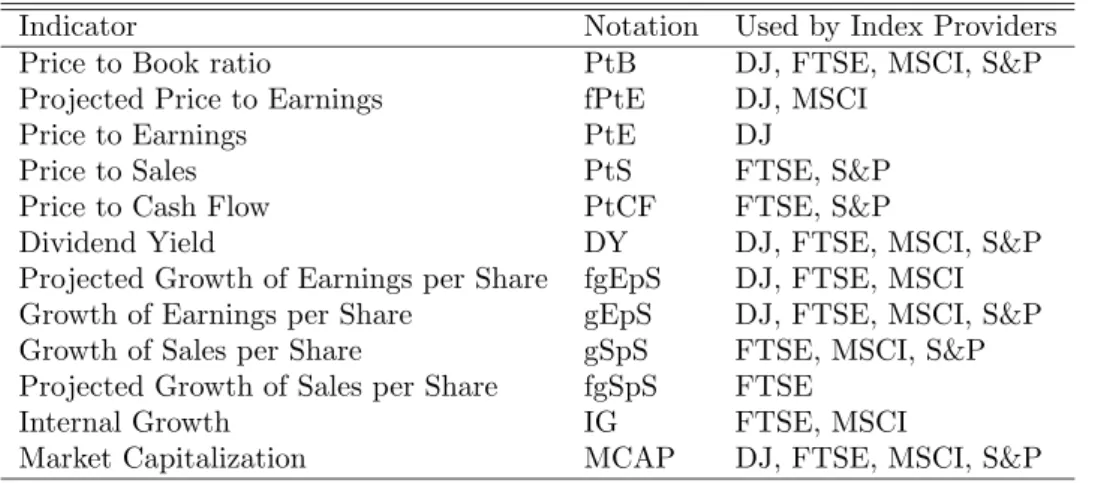
The set of explicative variables includes a group of ratios of price to fun-damental accounting characteristics, measuring companies’ performance: book value (PtB), earnings (PtE), sales (PtS) and price-to-cash flow (PtCF). Accompanied by the dividend yield (DY), they form a set of “value” factors, commonly used by market practitioners. Choosing accounting fundamentals we were largely inspired by the lists of the factors, use by global style index providers (see Table 1). It is noteworthy that index providers define separate dimensions for value and growth (except DJ STOXX), i.e. different sets of indicators are used to construct value and growth portfolios. On the contrary Fama and French (1993, 1996) and Lakonishok et al. (1994) refer to growth stocks as those, which are not value (i.e. low PtB for value and high PtB for growth). The rationale for this approach is that high market value relative to fundamentals implies high future growth rate, projected by rational investors.
We use direct measures of growth, computed over 1, 3 and 5 years: growth of sales-per-share (gSpS, gSpS3, gSpS5) and growth of earnings-per-share (gEpS,
gEpS3, gEpS5). Motivated by the market practice, we add a set of forecasts,
representing the consensus of financial analysts over future companies’ perfor-mance: forecast of growth of earnings-per-share over one year (fgEpS), fore-cast of long term growth of earnings-per-share (fgEpS5) and projected
price-Table 1: Accounting Fundamentals used as Style Factors
Indicator Notation Used by Index Providers Price to Book ratio PtB DJ, FTSE, MSCI, S&P Projected Price to Earnings fPtE DJ, MSCI
Price to Earnings PtE DJ
Price to Sales PtS FTSE, S&P Price to Cash Flow PtCF FTSE, S&P
Dividend Yield DY DJ, FTSE, MSCI, S&P Projected Growth of Earnings per Share fgEpS DJ, FTSE, MSCI Growth of Earnings per Share gEpS DJ, FTSE, MSCI, S&P Growth of Sales per Share gSpS FTSE, MSCI, S&P Projected Growth of Sales per Share fgSpS FTSE
Internal Growth IG FTSE, MSCI
Market Capitalization MCAP DJ, FTSE, MSCI, S&P
Growth variables can be computed over different time horizons, as explained in the text.
to-earnings (fPtE). All forecasts come from IBES. We also use the indicator of internal growth (IG, IG5), which is the reinvested part of the return-on-equity
(ROE). This indicator is used by many index providers. It is computed as (1-PR)×ROE where PR is the dividend payout ratio. For IG5 five-years average
is taken. The size factor is as usually captured by the market capitalization (MCAP).
Finally, we use past returns over one month, one quarter and one year to represent the so-called price momentum (PM1m, PM1q, PM1y). There is much
empirical evidence in favor of the predictive power of such variables. (Jegadeesh, 1990) evidence for the mean-reversion in monthly returns returns and thus prof-itability of short-term contrarian strategies. Jegadeesh and Titman (1993a) find outperformance for portfolios of stocks with high historical 3-month and yearly returns. Carhart (1997) add one-year momentum as a risk factor in the Fama and French framework to construct a four-factor model. Though momentum has nothing to do with the accounting fundamentals, we include it in the anal-ysis along with the value and growth factors mainly in order to see, whether its effect is persistent once these factors are controlled for.
For robustness purposes all factors are pre-processed using the probability integral transform, which enables mapping to a range from zero to one. So we do not consider absolute values of indicators, but only the relative ranking of stocks. This secures that the impact of outliers on the results is minimal.
The actual number of stocks included in the samples depends on the avail-ability of data for particular periods and for various indicators. It ranges from 408 for the long term historical growth of indicators in the early 80’es to about 1,200 for most variables in the recent years.
4
Formal Description of the Methodology
The three-factor model implies that stock returns’ premia in a cross-section can be explained by three variables, representing their sensitivities to the market portfolio (traditional CAPM beta) and two other artificially constructed risk factors: SMB (Small Minus Big) and HML (High Minus Low). The latter are proxied by the difference in returns of two portfolios: one including stocks with high values of PtB and MCAP and the other - stocks with low values of these characteristics.
Formally, for any period t and each stock i, the following regression equation is supposed to be verified:
ri,t− r f t = β
m
i,t δt+ βi,tPtBγPtBt + βi,tMCAPγMCAPt + εi,t (1)
where ri,t is the total return (capital gain and dividend yield) on stock i for
period t, rft is a risk-free interest rate; δtis the return premium on the market
portfolio at period t; βm
i,t is the traditional CAPM beta of stock i, which is
allowed to vary in time; γθ
t is the return premium on the factor, constructed
using the characteristic θ, which is PtB or MCAP; βθ
i,tis the sensitivity of stock
i returns to this factor and εi,t is an error term, assumed to be iid normal in
the cross-section.
One way to check the goodness of (1), inspired by the tests of CAPM in Friend and Blume (1970) and Black (1972), is to estimate the model
ri,t = ct+ βi,tmδt+ βPtBi,t γtPtB+ βi,tMCAPγtMCAP+ εi,t (2)
and then check that bct is close to rtf. Besides, if rtm, rtPtB and rMCAPt denote
returns on the market portfolio and portfolios, mimicking SMB and HML factors respectively and these quantities are observable1, we can check if the estimates
of premia from (2) correspond to their observed counterparts. So the equalities to be tested are: b ct= r f t (3) b δt= rmt − r f t b γPtB t = rtPtB− r f t b γMCAP t = rtMCAP− r f t
The cross-sectional regression (3) is estimated by OLS for each month. We use monthly returns on the 3-months US Treasury bills as risk-free rates of re-turns. Market portfolio return is proxied by the capitalization-weighted average of all returns on stocks, quoted at NYSE. SMB and HML are constructed with a threshold of 20% both from the top and the bottom of the distribution of PtB and MCAP. Unlike many other authors, we do not use the data for SMB and HML portfolios available on Kenneth French’s website but compute them ourselves in order to obtain factors representative of our sample.
1Neither market portfolios, nor the factors corresponding to SMB and HML are really
ob-servable. But for the three-factor model to be of any use, we need to be able to proxy for them. This is done further, when sensitivities to factors are estimated. Thus the tests, discussed here, check for the goodness of the model itself and of the factor proxies simultaneously, the two being inalienable.
Since the sensitivities βm
i,tand βiθare unobservable, they have to be estimated
prior to (2). To this end we use a three-factor time series model for each stock i, defined over a historic period [t − L; t]. It is given by the following equation, verified at each date t − l : l ∈ {1, . . . , L} :
ri,t−l− rft−l= βiPtBγPtBt−l + βiMCAPγt−lMCAP+ β m
i δt−l+ νi,t−l (4)
with νi,t−l a Gaussian white noise and all other notation unchanged. When the
portfolios, used for computing γθ
t−l, are constructed, the lag of 4 months for
θ is used. Historical period of 4 years (L = 48 months)2 for estimating (4) is
chosen. So sensitivities in (2) are estimated on the moving windows preceding the month, for which the cross-sectional regression (2) is estimated by OLS, so that there is no overlapping.
An alternative model, proposed by Daniel and Titman (1997), explains the excess return for each stock by the lagged characteristics of the issuing company and reads:
ri,t− rft = βi,tδt+ btPtB PtBi,t−l+bMCAPt MCAPi,t−l+εi,t (5)
where bθ
t is the return premium on the characteristics θ (PtB or MCAP), taken
with lag l, and all other notation remains unchanged. The lag is chosen to be 4 months, which enables that the information about accounting fundamentals is available to all market participants3.
As in the previous case we exclude the risk-free rate from (5) and estimate: ri,t= ct+ βi,tδt+ btPtB PtBi,t−l+bMCAPt MCAPi,t−l+εi,t (6)
and test the equalities:
bct= rft (7)
b
δt= rtm− r f t
Regression (6) is estimated by OLS for each month.
The sensitivity of each stocks’ returns to the market portfolio βi,tis used as a
control variable and is computed prior to the estimation of (5) from an ordinary CAPM time series regression for the months {t − L, . . . , t − 1} separately for each stock i: ri,t−l− rt−lf = βm i (r m t−l− r f t−l) + νi,t (8)
The length of the moving window for the estimation is 4 years, similar to equa-tion (4).
Models (6) and (2) are first estimated for all dates on the whole sample of stocks. Conditions (6) and (2) are tested and predictive power of the models is compared. Then estimations are repeated for reduced samples of stocks, whose betas do not match with characteristics according to the procedure, discussed in section 2. Thus we verify whether returns behave according to what companies’ characteristics or betas imply, which allows discriminating between the two models.
2
We use minimum 24 months for the first years of the sample where little data is available.
3
Firms are required to file their reports with the SEC no later than in 90 days from the fiscal year end, but there is evidence that considerable part of the companies do not comply (Fama and French, 1992)
Finally, we estimate augmented regression models of the form:
ri,t= ct+ βi,tmδt+ βi,tPtBγtPtB+ βi,tMCAPγtMCAP+ K X k=1 bk tθ k i,t−lεi,t (9) with θk
i,t−l, k = {1, . . . , K} lagged characteristics from Table 1. Various
combi-nations of accounting fundamentals are used and the significance of coefficients bk
t, βi,tm, βi,tPtB and βi,tMCAP is tested. If the three-factor model is true, only βi,tm,
βPtB
i,t and βMCAPi,t are expected to be systematically significant. This model is
also estimated in a restricted version, when Fama and French betas are omitted.
5
Discussion of the Results
We start with the tests, comparing regression estimates of risk factor premia with the observed premia. The series of tests (3) for the Fama and French model are estimated for 288 monthly periods on a sample of NYSE stocks, whose size progressively increases from 504 to 1614. As for the market portfolio premium, associated with CAPM beta, the equality of the estimated and observed premia is rejected at 0.9 confidence level in 53% of periods, for the size prenium in 57% of periods and for the value premium in 51% of periods . The observation that the constant in the regression is often different from the risk-free rate can be interpreted as the presence of a time-specific shock in stock returns that does not undermine the factor model concept. However, the results for the factor premia clearly suggest that the model is misspecified. For the alternative specification (5) the tests (7) reject the equality of the estimated and observed risk premia in 57% of periods and the equality of the estimated constant to the risk-free rate in 75% of periods.
All tested hypotheses are based on the idea that systematic risk factors are well represented by historical covariances with some portfolios of stocks. We question the adequacy of the assumption that these portfolios do mimic these systematic risk factors well, at least on individual stocks’ level. Note that the conclusion on misspecification of particular factors does not necessarily mean the rejection of the systematic risk story as whole. We rather suppose that sen-sitivity to systematic risk factors can be measured in another way. For example, accounting fundamentals of companies may better reflect companies’ exposure to different risks than historical correlations. The importance of fundamentals can also be justified outside the risk factor models by arguments of behavioral finance. Whatever the theoretical argument, our main interest is the practi-cal usefulness of historipracti-cal sensitivities and fundamentals in predicting stocks’ returns in a cross-section.
Our next test aims to detect, whether the effect of Fama and French historical betas have predictive power on returns because they are correlated to companies’ fundamentals or they are significant in themselves.
As described in the previous sections, we estimate regression models, corre-sponding to (1) and (5), on the full sample and on the reduced sample, including 30% of stocks, for which betas to HML and PtB values do not match. The results are given in Table 2. The table aggregates the estimates from 289 regressions for monthly periods. The full sample includes from 504 to 1614 stocks depending on the periods. The first two blocks of the table contain estimations, obtained
on the full sample for betas and characteristics. The last two correspond to the reduced samples. Correlation between betas and characteristics that is posi-tive (0.22) in the original sample becomes significantly negaposi-tive in the reduced samples (-0.53).
The first column of the table contains the percentage of time periods, for which the explicative variables were significant at 0.9 confidence level. The next two decompose the previous indicator into periods of positive and negative significant impact (in percentage of periods of significant impact). The aver-age value of the regression coefficients quantifies the magnitude of the factors’ impact. The latter is reported for the overall sample and for the positive and negative premia separately. An important question is whether the impact of factors is stable in time or reverses chaotically. The average number of months, for which the signs of the estimated regression slopes do not change, serves as a descriptive measure of such persistence. The duration of positive and negative runs is also computed separately in order to capture the asymmetric effects. The run test (Wald and Wolfowitz, 1948) checks for the randomness of the se-quences of positive and negative impacts (mutual independence of two outcomes is tested regardless of their unconditional probabilities). The periods of stable impact, lasting for more than one quarter, are of special importance, because they are more likely to be related to non-random aggregate economic factors, and because they can be easier analyzed and exploited in portfolio management. We observe that the direction of impact changes for the betas models, when the sample is reduced, while for the characteristics model it remains the same. So the effect due to characteristics completely dominates the impact of betas. The hypothesis that style premium in reality is associated with the fundamental PtB characteristic rather than with sensitivity to HML factor finds its support. Similar results were obtained for the impacts of βMCAP
i,t and MCAP on the
full and reduced sample (not reported here). Also note that the impact of factors in time is rather unstable, except, to some extent, the impact of the PtB characteristic.
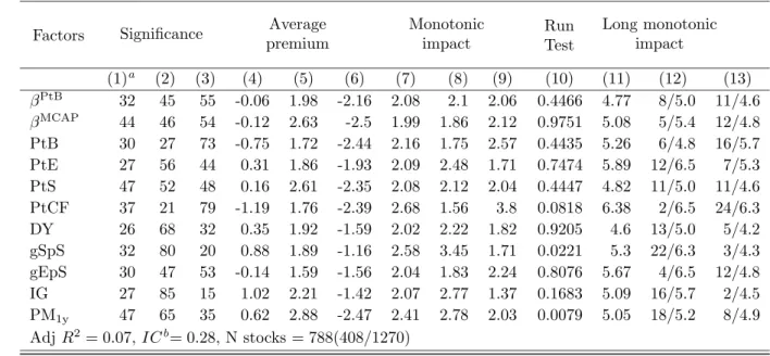
At the next stage we add a wide set of accounting fundamentals, listed in table (1)4 to the explicative variables of the Fama and French model and run
a series of regressions, corresponding to equation (9). The aggregated results of estimation are given in Table 3. The first immediate conclusion from the observation of the figures in the first three columns is that many accounting fundamentals are at least as significant as Fama and French factors and in several cases (PtS, PtCF, PM1y) are significant more often. Second, note that
the occurence of positive premia on βPtBand βMCAPis only slightly asymmetric.
Stocks with low βPtB (high sensitivity to HML factor) outperform in 55% and
underperform in 45% of periods, when significant premium is recorded. For many of the accounting fundamentals (PtB, PtCF, DY, gSpS, IG) and for price momentum the asymetry is much more pronounced.
In terms of the size of the average premium the fundamentals of value (PtB, PtS, PtCF) are also at least as good as the beta to HML. On the conrary, PtE is less important in predicting returns. The impact of various growth character-istics (gSpS, gEpS,IG) is very heterogeneous. Internal growth, measuring the
4
We only report the results for those variables that are of particular interest, i.e. for those that have significant impact on returns in more than 25% of periods. Other results are available on request. MCAP characteristic could not be included in this regression due to strong correlation with βMCAP
reinvested part of companies’s performance, comes out as one of the strongest factors of style performance. Though it is significant in only 27% of periods, positive impact clearly prevails (85% of all significant impacts). The average style premium per centile is 2.41bp, which is higher than the absolute value of the negative premimum on both βPtB and PtB itself. Growth of sales over
the past year (gSpS) is also important and positive impact dominates, though the magnitude of the average premium is less impressive. However, it is well clustered. The impact of growth of earnings is rather weak and does not have a prevailing direction.
We also tried to use longer time lags when computing growth indicators, but their predictive power deteriorated (not reported here). So recent accounting data are of greater relevance for forecasting returns than long-term average tendencies. Recent accounting fundamentals may better proxy changes in risk sensitivities of companies and in returns prospects that drive price fluctuations. For the momentum factors we find the results, consistent with Jegadeesh and Titman (1993b), i.e. negative but not significant impact of the returns over the past month/quarter (not reported in the table), and positive impact of the returns over the previous year. Clustering effect is for yearly momentum.
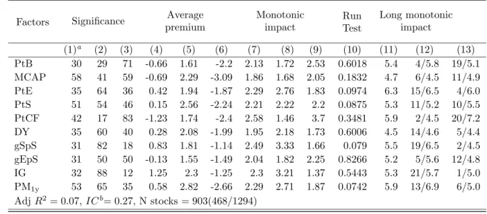
In table 4 we report the results of similar regressions, but when Fama and French betas are omitted. Size factor here is represented directly by market capitalization (MCAP). Its impact on returns appears to be stronger and more stable than that of βMCAP
i,t , reported in the previous regression. Globally, the
quality of regressions and predictive power remain the same. The separation between positive and negative impacts becomes more clear. Thus inclusion of βPtB and βMCAP
i,t does not significantly reduce the premia, associated to
accounting fundamentals and does not add much to the forecasting power of the model.
Table 2: Results of Regressions: Standard Models, Full and Reduced Samples.
Factors Significance Average premium Monotonic impact Run Test Long monotonic impact (1)a (2) (3) (4) (5) (6) (7) (8) (9) (10) (11) (12) (13) Three-factor model: Adj R2= 0.03, ICb
= 0.16, N stocks = 997(504/1614)
βPtB 47 37 63 -0.63 2.42 -2.91 2.1 1.78 2.43 0.5514 5.61 5/4.8 12/6.4
βMCAP 53 43 57 -0.38 2.99 -3.12 2.18 1.95 2.41 0.1722 5.01 8/4.9 14/5.14
Three-characteristics model: Adj R2= 0.03, IC = 0.18, N stocks = 921(441/1477)
PtB 52 34 66 -0.76 2.52 -2.63 2.37 1.72 3.02 0.1056 5.44 6/4.7 19/6.2 MCAP 58 45 55 -0.43 2.73 -3.27 2.04 1.93 2.14 0.7132 4.82 7/4.6 13/5.1 Reduced sample: three-factor model: Adj R2= 0.03, IC = 0.18, N stocks = 260(111/433)
βPtB 34 57 43 0.34 4.15 -3.53 2.04 2.04 2.04 0.6373 5.75 8/5.4 5/6.2
βMCAP 28 58 41 -0.21 3.5 -3.87 1.86 1.86 1.88 0.2876 7.86 7/4.7 10/5.0
Reduced sample: three-characteristics model: Adj R2= 0.03, IC = 0.19, N stocks = 269(121/444)
PtB 29 35 65 -0.87 2.81 -3.48 2.22 1.88 1.84 0.2606 5.78 7/5.4 15/6.3 MCAP 31 47 50 -0.32 3.43 -4.2 1.86 1.92 2.07 0.9661 4.94 9/4.9 10/5.0
a
(1) Periods when variable is significant, %; (2),(3) positive and negative impact, % of significant values; (4),(5),(6) duration of monotonic impact, months: average, positive, negative; (7) run test, p-value; (8),(9),(10) average, positive and negative premium per centile, bp; (11) long ( >1Q) periods with monotonic impact: average duration, months; (12),(13) positive and negative monotonic impact: nb of periods/average duration.
b
Information coefficient
Table 3: Three-factor Model Augmented with Accounting Fundamentals.
Factors Significance Average premium Monotonic impact Run Test Long monotonic impact (1)a (2) (3) (4) (5) (6) (7) (8) (9) (10) (11) (12) (13) βPtB 32 45 55 -0.06 1.98 -2.16 2.08 2.1 2.06 0.4466 4.77 8/5.0 11/4.6 βMCAP 44 46 54 -0.12 2.63 -2.5 1.99 1.86 2.12 0.9751 5.08 5/5.4 12/4.8 PtB 30 27 73 -0.75 1.72 -2.44 2.16 1.75 2.57 0.4435 5.26 6/4.8 16/5.7 PtE 27 56 44 0.31 1.86 -1.93 2.09 2.48 1.71 0.7474 5.89 12/6.5 7/5.3 PtS 47 52 48 0.16 2.61 -2.35 2.08 2.12 2.04 0.4447 4.82 11/5.0 11/4.6 PtCF 37 21 79 -1.19 1.76 -2.39 2.68 1.56 3.8 0.0818 6.38 2/6.5 24/6.3 DY 26 68 32 0.35 1.92 -1.59 2.02 2.22 1.82 0.9205 4.6 13/5.0 5/4.2 gSpS 32 80 20 0.88 1.89 -1.16 2.58 3.45 1.71 0.0221 5.3 22/6.3 3/4.3 gEpS 30 47 53 -0.14 1.59 -1.56 2.04 1.83 2.24 0.8076 5.67 4/6.5 12/4.8 IG 27 85 15 1.02 2.21 -1.42 2.07 2.77 1.37 0.1683 5.09 16/5.7 2/4.5 PM1y 47 65 35 0.62 2.88 -2.47 2.41 2.78 2.03 0.0079 5.05 18/5.2 8/4.9 Adj R2= 0.07, ICb = 0.28, N stocks = 788(408/1270) a
(1) Periods when variable is significant, %; (2),(3) positive and negative impact, % of significant values; (4),(5),(6) average, positive and negative premium per centile, bp; (7),(8),(9) duration of monotonic impacts: average, positive and negative, months; (10) run test, p-value; (11) long ( >1Q) periods with monotonic impact: average duration, months; (12),(13) positive and negative monotonic impact: nb of periods/average duration.
b
Information coefficient
Table 4: Characteristics Model with Multiple Accounting Fundamentals.
Factors Significance Average premium Monotonic impact Run Test Long monotonic impact (1)a (2) (3) (4) (5) (6) (7) (8) (9) (10) (11) (12) (13) PtB 30 29 71 -0.66 1.61 -2.2 2.13 1.72 2.53 0.6018 5.4 4/5.8 19/5.1 MCAP 58 41 59 -0.69 2.29 -3.09 1.86 1.68 2.05 0.1832 4.7 6/4.5 11/4.9 PtE 35 64 36 0.42 1.94 -1.87 2.29 2.76 1.83 0.0974 6.3 15/6.5 4/6.0 PtS 51 54 46 0.15 2.56 -2.24 2.21 2.22 2.2 0.0875 5.3 11/5.2 10/5.5 PtCF 42 17 83 -1.23 1.74 -2.4 2.58 1.46 3.7 0.3481 5.9 2/4.5 20/7.2 DY 35 60 40 0.28 2.08 -1.99 1.95 2.18 1.73 0.6006 4.5 14/4.6 5/4.4 gSpS 31 82 18 0.83 1.81 -1.14 2.49 3.33 1.66 0.079 5.5 19/6.5 2/4.5 gEpS 31 50 50 -0.13 1.55 -1.49 2.04 1.82 2.25 0.8266 5.2 5/5.6 12/4.8 IG 32 88 12 1.25 2.3 -1.25 2.3 3.21 1.37 0.5443 5.3 21/5.7 1/5.0 PM1y 53 65 35 0.58 2.82 -2.66 2.29 2.71 1.87 0.0742 5.9 13/6.9 6/5.0 Adj R2= 0.07, ICb = 0.27, N stocks = 903(468/1294) a
(1) Periods when variable is significant, %; (2),(3) positive and negative impact, % of significant values; (4),(5),(6) average, positive and negative premium per centile, bp; (7),(8),(9) duration of monotonic impacts: average, positive and negative, months; (10) run test, p-value; (11) long ( >1Q) periods with monotonic impact: average duration, months; (12),(13) positive and negative monotonic impact: nb of periods/average duration.
b
Information coefficient
6
Conclusion
We studied the predictive power of fundamental performance characteristics on future stock returns, using a large sample of stocks, quoted on NYSE since 1979. Our results suggest that several fundamental characteristics can be potential candidates to represent style factors. We find that, along with the price-to-book and price-to-earnings factors, traditionally studied in the “value puzzle” academic literature, other variables (internal growth, past sales growth, price-to-sales, dividend yield, etc.) have important predictive power of future returns and generate considerable premia. Some variables are significant over many time periods, but no long-term effect is recorded because the direction of their impact varies in time. These results are consistent with the common practice of using several characteristics to define investment styles.
The most influential three-factor model (Fama and French, 1993), incorpo-rating price-to-book and market capitalization in the equilibrium market re-turns, suggests that their impact comes through the covariance of returns with hidden risk factors, represented by the “High minus Low” book-to-price and the “Small Minus Big” market cap portfolios. The adequacy of this framework was first questioned by Daniel and Titman (1997). We report extensive evidence that the artificial risk factors approach is not sufficient, at least for predicting returns at individual stock’s level. We show that fundamental characteristics themselves contain much more information for predicting the cross-section of future returns.
In our view, the fact that individual companies’ characteristics explain stock returns does not automatically imply the absence of underlying systematic risk factors. Companies, ranking high or low according to a particular indicator, can be more sensitive to some economic variables or conditions than other stocks are, so that fundamental indicators themselves are better proxies for the stock returns’ sensitivity to risk factors, than the corresponding betas. The switching of long-lasting periods, characterized by outperformance or underperformance of style-based portfolios, is an evidence in favor of the link between style per-formance and economic risk factors.
Our findings are relevant for practical applications, related to the estimation of cost of capital, and for constructing style-based market timing investment strategies. Besides, they can be used for designing style indices as an empirical background for choosing fundamentals, driving performance. A natural further development would be to study the predictive power of multifactor style scores, determined as a linear combination of different variables in a way that it is done by index providers.
References
W. Banz. The relationship between return and market value of common stocks. Journal of Financial Economics, 9(1):3–18, 1981.
J. Bartholdy and P. Peare. Estimation of expected return: Capm vs. fama and french. International Review of Financial Analysis, 14(4):407–427, 2005. S. Basu. The relationship between earnings yield, market value, and return for
nyse common stocks: Futher evidence. Journal of Financial Economics, 12: 129–156, 1983.
F. Black. Capital market equilibrium with restricted borrowing. Journal of Business, 45:444–455, 1972.
M. Carhart. On persistence in mutual fund performance. Journal of Finance, 52(1):57–82, 1997.
L. Chan and J. Lakonishok. Value and growth investing: Review and update. Financial Analysts Journal, 60(1):71–86, 2004.
K. Daniel and S. Titman. Evidence on characteristics of cross sectional variation in stock returns. Journal of Finance, 52(1):1–33, 1997.
K. Daniel, S. Titman, and K. Wei. Explaining the cross-section of stock returns in japan: Factors or characteristics? Journal of Finance, 56(2):743–766, 2001. J. Davis, E. Fama, and K. French. Characteristics, covariances, and average
returns: 1929 to 1997. Journal of Finance, 55(1):389–406, 2000.
W. De Bondt and R. Thaler. Further evidence on investor overreaction and stock market seasonality. Journal of Finance, 42(3):557–581, 1986.
E. Fama and K. French. The cross-section of expected stock returns. Journal of Finance, 53(6):427–465, 1992.
E. Fama and K. French. Common risk factors in the returns on stocks and bonds. Journal of Financial Economics, 33:3–56, 1993.
E. Fama and K. French. Multifactor explanations of asset pricing anomalies. Journal of Finance, 51(1):55 – 84, 1996.
I. Friend and M. Blume. Measurement of portfolio performance under uncer-tainty. American Economic Review, 60(4):561–575, 1970.
N. Jegadeesh. Evidence of predictable behavior of security returns. Journal of Finance, 45(3):881–898, 1990.
N. Jegadeesh and S. Titman. Returns to buying winners and selling losers: Implications for stock market efficiency. Journal of Finance, 48(1):65–91, 1993a.
N. Jegadeesh and S. Titman. Returns to buying winners and selling losers: Implications for stock market efficiency. Journal of Finance, 48(1):65–91, 1993b.
J. Lakonishok, A. Shleifer, and R.Vishny. Contrarian investment, extrapolation, and risk. Journal of Finance, 49(5):1541–1578, 1994.
J. Litner. The valuation of risk assets and the selection of risky investments in stock portfolios and capital budgets. Review of Economics and Statistics, 47 (1):13–37, 1965.
B. Rosenberg, K. Reid, , and R. Lanstein. Persuasive evidence of market ineffi-ciency. Journal of Portfolio Management, 11:9–17, 1995.
W. Sharpe. Capital asset prices: A theory of market equilibrium under condi-tions of risk. Journal of Finance, 19(3):425 – 442, 1964.
A. Wald and J. Wolfowitz. Optimum character of the sequential probability ratio test. The Annals of Matematical Statistics, 19(3):326–339, 1948.