HAL Id: hal-00614974
https://hal.archives-ouvertes.fr/hal-00614974
Submitted on 17 Aug 2011HAL is a multi-disciplinary open access archive for the deposit and dissemination of sci-entific research documents, whether they are pub-lished or not. The documents may come from teaching and research institutions in France or abroad, or from public or private research centers.
L’archive ouverte pluridisciplinaire HAL, est destinée au dépôt et à la diffusion de documents scientifiques de niveau recherche, publiés ou non, émanant des établissements d’enseignement et de recherche français ou étrangers, des laboratoires publics ou privés.
National Travel Survey 2007-08
Sophie Roux, Jimmy Armoogum
To cite this version:
Sophie Roux, Jimmy Armoogum. Analysis bias due to survey non response in the French National Travel Survey 2007-08. 12th World Conference on Transport Research, Jul 2010, Lisbonne, Portugal. 14p. �hal-00614974�
ANALYSIS OF BIASES DUE TO SURVEY
NON RESPONSE IN THE FRENCH
NATIONAL TRAVEL SURVEY 2007-08
ROUX Sophie
Institut national de recherche sur les transports et leur sécurité (INRETS)
Département Economie et Sociologie des transports (DEST)
Centre de Recherche de l’Institut de Démographie de l’Université Paris I (CRIDUP)
Bâtiment Descartes 2
2, rue de la Butte Verte
F-93166 Noisy le Grand cedex
Tel : +33 (0)1.45.92.55.87
sophie.roux@inrets.fr
ARMOOGUM Jimmy
Institut national de recherche sur les transports et leur sécurité (INRETS)
Département Economie et Sociologie des transports (DEST)
Bâtiment Descartes 2
2, rue de la Butte Verte
F-93166 Noisy le Grand cedex
Tel : +33 (0)1.45.92.55.79
jimmy.armoogum@inrets.fr
ABSTRACT
While nonresponse results in a reduced sample size, a more important concern of researchers is the possible impact of nonresponse bias. Bias is introduced when those that do not respond to the inquiry are systematically different from those that do respond on key estimates. In this circumstance, as the above section describes, the response mechanism is “confounded” with characteristics of the sample units. For example, if nonrespondents tended to take more trips, or longer trips than respondents, the estimates of travel produced from only survey respondents will be too low and not representative of the whole population (only those that responded).
Getting the advantage that for the last French National Travel Survey (FNTS) 2007-2008 the sample was drawn directly from the census and the list of new residences built since the census, and therefore we have lots of information about respondent and non-respondent to the different survey instruments in the FNTS. We will quantify these biases by using auxiliary information in different calibration that we will produce.
INTRODUCTION
All surveys are susceptible to a variety of types of error that affect different parts of the survey process, have different implications for data quality and are amenable to different forms of prevention or compensation (Groves, 1989; Richardson et al., 1995; Zimowski et al. 1997). Nonresponse errors are those generally associated with the failure of sample units to participate fully in the survey. It is usual to distinguish two different forms of nonresponse.
Unit nonresponse refers to the failure of a unit in the sample frame to participate in thesurvey. In the context of travel diary surveys, unit nonresponse can arise for a number of different reasons including refusal, non-contact, infirmity or temporary absence (see, e.g., Brög and Meyburg, 1980, Kim et al., 1993; Richardson and Ampt, 1994; Stopher and Stecher, 1993; Thakuriah et al., 1993).
Item nonresponse refers to the failure to obtain complete information from a participatingunit. In the context of travel diary surveys, the most significant form of item nonresponse is probably the under reporting of mobility due to respondents‟ failure to properly recall and/or record all the relevant journeys that they make (see, e.g., Ampt and Richardson, 1994; Brög and Meyburg, 1981; Brög et al., 1982, Hassounah et al., 1993). Item nonresponse can be regarded as a particular form of the more general problem of measurement error in survey research (Groves, 1989).
There is no justification for assuming that people who respond have the same characteristics as those who do not (Forsman et al., 2007). Thus, in computing estimates from the available data collected, we may face biases, whose size and direction of error are unknown. In order to show how these non-response problems can be solved, we will take as an example the daily trips in the French National Travel Survey 2007-08. Most of these solutions are rather general, but some aspects are specific to this case as the sample is drawn from the census, which allows the characterization of the households that refused to answer.
THE FRENCH NATIONAL TRAVEL SURVEY2007-08
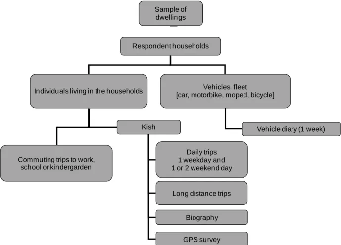
Once per decade, the Ministry of Transport and the National Institute of Statistics use to conducting a National Household Travel Survey with the scientific support of INRETS. It is the data source providing the most transverse and consistent overview of mobility, whatever the modes and the transport situations of people living in France may be. The aim of the French National Travel survey is the description of short and long distance trips made by households living in France, as well as their access to and use of public and private transport means. Figure 1 gives an overview of FNTS 2007-2008. The survey is organized around the three following topics: Description of trips; Vehicle ownership and use and accessibility to public transport.
Sample of dwellings
Respondent households
Individuals living in the households Vehicles fleet
[car, motorbike, moped, bicycle]
Kish
Daily trips 1 weekday and 1 or 2 weekend day Commuting trips to work,
school or kindergarden
Long distance trips
GPS survey
Vehicle diary (1 week)
Biography
Figure 1: Overview of the French National Travel Survey (FNTS 2007-2008).
Six survey instruments were used:
1. During the first visit a CAPI questionnaire is designed to collect at household level (including household members) the socio-demographic variables, characteristics of commuting trips to work, school or kindergarten; driving licenses and car use, traffic accidents; season tickets and discounts in public transport; description of vehicles available in the household and the housing environment;
2. A 7 days vehicle diary is attributed to one of the household's vehicles (selected with unequal probability distribution to give more chance to be drawn to motor two wheelers, which are particularly interesting on the point of view of road safety) to be filled by the vehicle users;
3. During the second visit, for one person above 6 years old, selected with unequal probability distribution giving more chance to highly mobile persons (within each households), is asked to describe her/his long distance trips made during the last three months (as recalled from memory);
4. The same person was asked to describe her/his trips made one weekday before the interview, and one weekend day (either Saturday or Sunday);
5. A sub-sample of approximately 1 100 individuals was asked to fill a biographical grid in order to describe the transport means used throughout their whole past life;
A sample size of about 30,000 dwellings (including 5 regional add-ons) was selected in the 1999 census and the list of new residences built since the census. The sample was spread over six waves covering 12 months, in order to neutralize the seasonal variations which affects mobility (especially for long distance travel).
Table 1 – Sample size and response rate
Number of dwelling drawn in the sample Number of dwelling out of the scope Number of Main dwelling Number of non-respondents households (2nd visit) Number of survey performed 30 165 4 272 25 893 7 261 18 632
Although the majority of residences in our sample are the main residence of a household, this is not always the case: among the 30 165 dwellings visited, 4 272 (14%) were out of the scope (vacant housing, second or occasional homes). Among the 25 893 selected households in the scope, 7 261 (28%) of them refused to respond to the 2nd visit of the survey.
THE RESPONSE MECHANISM
Among the 22 724 dwellings that were main household dwellings in the 1999 French census, we have some useful information allowing us to find out the probability for a household to respond to the survey, this is usually called the response mechanism. We built a logit model to detect the response mechanism because logit modeling shows the influence of each dimension “everything being equal in other respects". Although the household living in the selected dwelling could be different from those who lived there in 1999 (at the moment of the census), we consider them as equivalent. We compute the following variables for the response mechanism:
Zone of residence (people living in rural areas, people living in conurbation of less than 20 000 inhabitants, people living in conurbation from 20 000 to 100 000; people living in conurbation from 100 000 to Paris region; Paris conurbation);
Building belonging to the municipality with « low rents lodging »(yes; no); Type of dwelling (house and farm ; others types);
Dwelling with/without interphone (house; apartment with interphone; apartment without interphone);
Number of rooms of the dwelling (0-1 room ; 2-3 rooms ; 4-5 rooms ; 6 rooms and more);
Surface of the dwelling (less than 40m²; from 40 to 70 m²; from 70 to100 m²;from 100 to 150 m² ; more than 150 m²);
Size of the household at the 1999 census (1 person; 2 persons; 3 persons; 4 persons and more);
Age of the head of the household at the 1999 census (from 15 to 34 years old; from 35 to 49 years old; from 50 to 64 years old; from 65 years old and more);
Gender of the head of the household at the 1999 census (male; female); Household car fleet at the 1999 census (0 car, 1 car ; 2 cars and more);
Wave of survey (May – June 2007; July – August2007; September – October 2007; November – December 2007; January – February2008; March – April 2008).
Table 2 – Global significance analysis of the variables used in the Logit model
Effect DF Wald Chi-Square Pr > ChiSq
Zone of residence 4 47,65 <0,0001
Wave of survey 5 41,99 <0,0001
Age of the head of the household at the 1999 census 3 23,47 <0,0001 Household car fleet at the 1999 census 2 15,28 0,00
Number of rooms of the dwelling 3 10,07 0,02
Building belonging to the municipality with « low rents
lodging » 1 2,35 0,13
Type of dwelling 1 1,68 0,20
Surface of the dwelling 4 2,44 0,66
Dwelling with/without interphone 2 0,21 0,90
Gender of the head of the household at the 1999
census 1 0,02 0,90
Size of the household at the 1999 census 3 0,59 0,90
Source: INSEE-SOeS-INRETS, French National Travel Survey 2007-08
We computed a global significance analysis of the variables used in the Logit model, following the methodology in Gourieroux C. (2000), as the difference -2LogL-(-2LogL0) follows asymptotically a Chi-2 law. Among the variables we had with the census, the zone of residence, the wave of survey, the age of the head of the household at the census, the household car fleet at the census, and the number of rooms of the dwelling play a major role in the response mechanism. The other variables such as the building belonging to the municipality with « low rents lodging », the type of dwelling, the surface of the dwelling, the dwelling with/without interphone, the gender of the head of the household at the 1999 census, and the size of the household at the 1999 census are correlated with the probability to respond or not respond to the survey but adding them in the model do not add significant information (see table 2).
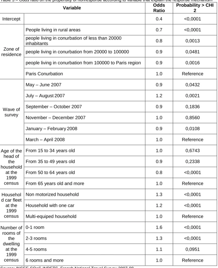
Table 3 – Odds ratio on the propensity of nonresponse according to variable that explain the response mechanism Variable Odds Ratio Probability > CHI 2 Intercept 0.4 <0,0001 Zone of residence
People living in rural areas 0.7 <0,0001
people living in conurbation of less than 20000
inhabitants 0.8 0,0013
people living in conurbation from 20000 to 100000 0.9 0,0481 people living in conurbation from 100000 to Paris region 0.9 0,0016
Paris Conurbation 1.0 Reference
Wave of survey May – June 2007 0.9 0,0432 July – August2007 1.2 0,0021 September – October 2007 0.9 0,1836 November – December 2007 1.0 0,8560 January – February2008 0.9 0,0108
March – April 2008 1.0 Reference
Age of the head of the household at the 1999 census
From 15 to 34 years old 1.0 0,6743
From 35 to 49 years old 0.9 0,2338
From 50 to 64 years old 0.8 <0,0001
From 65 years old and more 1.0 Reference
Househol d car fleet
at the 1999 census
Non motorized household 1.3 <0,0001
Household with one car 1.2 <0,0001
Multi-equiped household 1.0 Reference
Number of rooms of the dwelling at the 1999 census 0-1 room 1.6 <0,0001 2-3 rooms 1.3 <0,0001 4-5 rooms 1.1 0,0951
6 rooms and more 1.0 Reference
Source: INSEE-SOeS-INRETS, French National Travel Survey 2007-08
The odds ratio indicate the probability of the interviewees to be non-respondent by zone of residence, wave of survey, age of the household, household car fleet and number of rooms of the dwelling at the 1999 census.
Failures are more often in densely populated conurbations, indeed households living in densely area have an higher probability to be non-respondent than those living in rural areas;
Failures are more frequent during summer, a period during which we assume that households are more mobile (holidays,…). The risk to be non-respondent is 1.2 times higher among the households surveyed in July and August 2007 than among those surveyed in March and April 2008.
Failure rates are higher for households whose head is under 35 years and for those whose head is over 65 years.When the heads of households is aged from 35 to 65, we have a reduced risk of nonresponse compared to those aged 65 year old or those younger than 35.Most likely for different reasons, for the first group it emphasizes the difficulty for interviewer to reach these households and for the second group for the reluctance of older people to answer to long and burdensome questionnaire;
Non motorized households are less favorable to accept the survey. Indeed, households without any cars are 1.3 times more likely to be non-respondent in comparison to multi-equipped household;
Households living in a single room dwelling are 1.6 times more likely not to respond in comparison to households living in several rooms. Let‟s note that this variable is correlated with the number of people living in the household. Thus, a big household size is accompanied with a greater probability to respond;
The variables of the 1999 census which explain the response mechanism to the FNTS, often emphasize the difficulty of the interviewers to reach younger households, who are probably the most actives and the most mobile, and households living in the cities most densely populated, where there are more and more buildings equipped with interphone.
STRATEGIES TO CORRECT NONRESPONSE BIAIS
Calibration on margins is a weight-class method used when the total of each auxiliary information is known. Calibration on margins is an iterative process that adjusts certain sample totals or ratios, to make them match with certain corresponding totals or ratios that are known from the population. The calibration‟s methodology was developed by Deming and Stephan in the early 40‟s with the raking ratio process. We have used a software of calibration on margins called CALMAR2, which was developed by INSEE (Deville 2004; Le Guennec & Sautory 2003).
This stage is essential to ensure a representative sample and the comparison with some others statistics sources (for instance, other national surveys). The calibration on margins must be implemented on variables which explain (or are correlated with) transport behavior the variable that explain the nonresponse mechanism, and for which the total is accurately known (Deville, 1999). The population reference is ordinary households known by the rolling census.
When trying to reduce the impact of nonresponse bias by looking at known characteristics of nonrespondents and comparing them with those same characteristics of respondents. If differences in known characteristics are found between respondents and nonrespondents, weights can be developed that will reduce these biases. We had tested nine different calibrations to see the impacts of these weighting methods on the estimation of daily mobility. We choose the following margins from the census, as they are in the response mechanism
and/or correlated with mobility: the report day; professions and socioprofessional categories, age and gender, size of the households, wave of survey, motorisation, zone of residence. Let:
- W-ALL be the weight obtain by using a calibration all information (eg: the report day; professions and socioprofessional categories, age and gender, size of the households, wave of survey, motorisation, zone of residence);
- W-UR be the weight obtain by considering a uniform response mechanism (eg: the final weight is obtain by using an equal response rate);
- W-DAY be the weight using all available information in the calibration except the report day (eg: professions and socioprofessional categories; age and gender; size of the households; wave of survey; motorisation; zone of residence);
- W-PCS be the weight using all available information in the calibration except the professions and socioprofessional categories;
- W-AGG be the weight using all available information in the calibration except age and gender;
- W-SHH be the weight using all available information in the calibration except the size of the households;
- W-WAV be the weight using all available information in the calibration except the wave of the survey
- W-CAR be the weight using all available information in the calibration except the motorization;
- W-ZON be the weight using all available information in the calibration except the zone of residence
We consider that W-ALL is the best weight we can produce (as we use all auxiliary information we have). Let‟s compare the estimates of the number of individuals that the other weights give. In the Tables 4 to table 10 we show only the estimation of the number of individual for the W-ALL weight, the relative difference with W-UR for all variable in the calibration (where generally we have the deepest gap) and the difference with W-X where X is not in the calibration (it‟s not necessary to see the other tables because if the variable is in the calibration then we do not have any gap).
Table 4 – Gap between the estimation of number of individuals with W-ALL, W-UR and W-DAY
Weight used
W-ALL W-UR W-DAY
Number of individuals (in thousands) Relative difference with W-ALL Relative difference with W-ALL Reporting day Monday 11,298 -8% -7% Tuesday 11,298 0% 1% Wednesday 11,298 -5% -5% Thursday 11,298 -10% -10% Friday 11,298 20% 21%
Table 5 – Gap between the estimation of number of individuals with W-ALL, W-UR and W-PCS Weight used W-ALL W-UR W-PCS Number of individuals (in thousands) Relative difference with W-ALL Relative difference with W-ALL Professions and Socioprofessional Categories Farmer 1,436 24% 14% Craftsman/Tradesman 3,283 -10% -13% Intermediary active 10,020 5% 5% Intermediary retired 4,073 15% 6%
Blue collars active 14,769 0% 0%
Blue collars retired 8,565 -17% -25%
Unemployed 6,954 13% 18%
Between 6 and 14 years 7,392 -11% -1%
Source: INSEE-SOeS-INRETS, French National Travel Survey 2007-08
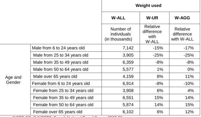
Table 6 – Gap between the estimation of number of individuals with W-ALL, W-UR and W-AGG
Weight used
W-ALL W-UR W-AGG
Number of individuals (in thousands) Relative difference with W-ALL Relative difference with W-ALL Age and Gender
Male from 6 to 24 years old 7,142 -15% -17%
Male from 25 to 34 years old 3,905 -25% -25%
Male from 35 to 49 years old 6,359 -8% -8%
Male from 50 to 64 years old 5,577 1% 0%
Male over 65 years old 4,159 8% 11%
Female from 6 to 24 years old 6,914 -8% -10%
Female from 25 to 34 years old 3,908 6% 4%
Female from 35 to 49 years old 6,551 15% 14% Female from 50 to 64 years old 5,874 14% 15%
Female over 65 years old 6,102 6% 12%
Table 7 – Gap between the estimation of number of individuals with W-ALL, W-UR and W-SHH Weight used W-ALL W-UR W-SHH Number of individuals (in thousands) Relative difference with W-ALL Relative difference with W-ALL Size of the household 1 person 8,696 1% 1% 2 persons 17,114 2% 1% 3 persons 10,603 -8% -7% 4 persons 11,477 3% 5%
5 persons and more 8,602 -4% -2%
Source: INSEE-SOeS-INRETS, French National Travel Survey 2007-08
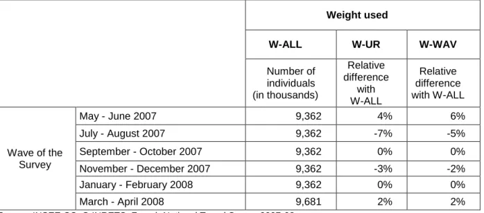
Table 8 – Gap between the estimation of number of individuals with W-ALL, W-UR and W-WAV
Weight used
W-ALL W-UR W-WAV
Number of individuals (in thousands) Relative difference with W-ALL Relative difference with W-ALL Wave of the Survey May - June 2007 9,362 4% 6% July - August 2007 9,362 -7% -5% September - October 2007 9,362 0% 0% November - December 2007 9,362 -3% -2% January - February 2008 9,362 0% 0% March - April 2008 9,681 2% 2%
Source: INSEE-SOeS-INRETS, French National Travel Survey 2007-08
Table 9 – Gap between the estimation of number of individuals with W-ALL, W-UR and W-CAR
Weight used
W-ALL W-UR W-CAR
Number of individuals (in thousands) Relative difference with W-ALL Relative difference with W-ALL Motorisation 0 car 7,385 2% 4% 1 car 24,046 -3% -2% 2 cars or more 25,062 1% 0%
Table 10 – Gap between the estimation of number of individuals with W-ALL, W-UR and W-ZON
Weight used
W-ALL W-UR W-ZON
Number of individuals (in thousands) Relative difference with W-ALL Relative difference with W-ALL Zone of residence
Rural municipalities in a non rural
area 7,811 12% 13%
Rural municipalities in a rural area 6,512 -1% -1% City center of conurbation less
then 19 999 inhabitants 7,979 -2% -1%
Suburbs of conurbation less than
19 999 inhabitants 1,475 16% 16%
City center of conurbations 20 000
to 49 999 inhabitants 2,493 -20% -19%
Suburbs of conurbations 20 000 to
49 999 inhabitants 977 2% 4%
City center of conurbations 50 000
to 99 999 inhabitants 2,510 -16% -14%
Suburbs of conurbations 50 000 to
99 999 inhabitants 1,361 11% 11%
City center of conurbations
100 000 to 199 999 inhabitants 1,753 -9% -6% Suburbs of conurbations 100 000
to 199 999 inhabitants 1,322 8% 14%
City center of conurbations
200 000 to 1 999 999 inhabitants 5,674 -8% -7% Suburbs of conurbations 200 000
to 1 999 999 inhabitants 7,090 0% 1%
City center of the Paris region 2,016 0% -3%
Suburbs of the Paris region 7,520 -1% -2%
Source: INSEE-SOeS-INRETS, French National Travel Survey 2007-08
The daily mobility is measured with a face to face interview by the description of the mobility made the day before. The protocol does not impose any particular weekday, as the interviewer and the interviewees choose the day of the visit. The relative difference with W-ALL and W-UR confirms that interviewers have difficulties to collect data on households on Mondays and Thursdays. They have therefore more complicatedness to contact households on Tuesday and on Friday. In contrast, Friday is the most describe day, as respondents are more willing to meet interviewers on Saturday. The relative difference with W-ALL and W-UR and W-ALL and W-DAY give similar results for each day. When we remove the "report day" off the calibration, the other variables of the calibration do not adjust properly at the distribution of survey days, e.g 20% for each day. If we use DAY we will have some bias in our estimations (the gap W-DAY and W-ALL is not negligible), it is necessary to introduce the reporting day in the calibration.
This is also true for the wave of the survey. As the interviewees are less accessible at their home in summer (probably for holidays), the response rate is lower in July and August. If we use W-WAV we will have some bias in our estimations (the gap W-WAV and W-ALL is not negligible), it is necessary to introduce the wave of the survey in the calibration.
The relative difference with W-ALL and W-AGG shows to us that interviewees are more often woman aged 35 to 65 and less often men aged 6 to 35. When we remove the "age and gender" of the calibration, the other variables of the calibration do not adjust properly the distribution by age and gender. There is no correlation between the variable "age and gender" and the other variables, it is therefore necessary to introduce the information age and gender in the calibration.
The relative difference with W-ALL and W-UR and W-ALL and W-PCS give different results. When we remove the "Professions and Socioprofessional Categories" off the calibration, the other variables of the calibration do not compensate properly the distribution of the "Professions and Socioprofessional Categories". The "Professions and Socioprofessional Categories" must be part of the variable calibration.
IN TERM OF MOBILITY
Table 11 – Gap between the estimation of number of average trips by day with W-ALL, W-X
Mean of the number of
trips per day
Relative difference with W-ALL
W-ALL W-UR W-DAY W-PCS W-AGG W-SHH W-WAV W-CAR W-ZON 3,21 0,04% 0,05% 0,15% -0,23% 0,05% 0,04% -0,05% -0,30%
Source: INSEE-SOeS-INRETS, French National Travel Survey 2007-08
When we look at the number of trips per day for the overall population, the relative difference with W-ALL and all other weights we found similar results except for the "Professions and Socioprofessional Categories", "age and gender" and "zone of residence". For the first, the removal of this variable has the effect of slightly increasing the average number of trips per day. Conversely, the other two variables have the effect of decreasing the mean number of trips per day. The fact that the average number of trips per day is quite similar does not necessarily imply that people who did not respond had the same behaviour in terms of daily mobility. These means are the result of a play of compensation between those who have not responded because they do not perform trips and those who have not responded because they are very mobile.
CONCLUSION
The methods presented in this paper depend on the context of the survey. The analysis of the nonresponse mechanism for calibrations depends on the availability of an exhaustive and up to date sampling base. Working with our National Institute of Statistics, we had the opportunity, of drawing the sample from the census. This is not always the case, as in certain countries, drawing samples from the census is forbidden for privacy reasons. We found that the best explanatory factors of total nonresponse are the zone of residence, the survey period, age &
gender of the head of the households, the households car fleet and the size of the households. It is important to minimize the biases due to measurement errors by a calibration on margins using the variables that play a role in the response mechanism.
REFERENCES
Adler, T. J. (2003): Reducing the Effects of Item Nonresponse in Transport Surveys, in Transport Survey Quality and Innovation, Elsevier Science Ltd., Kidlington, Oxford, United Kingdom.
Ampt, E. and Richardson, A. (1994) „The validity of self-completion surveys for collecting travel behaviour data‟, Proceedings 22nd European Transport Forum, PTRC, London.
Brög, W. and Meyburg, A. (1980) „The non-response problem in travel surveys - an empirical investigation‟ Transportation Research Record 775, 34-38.
Brög, W. and Meyburg, A. (1981) „Considerations of non-response effects on large scale mobility surveys‟ Transportation Research Record 807, 39-46.
Brög, W. Erl, E., Meyburg, A., Wermuth, M. (1982) „Problems of non-reported trips in surveys of nonhome activity patterns, Transportation Research Record 891, 1-5.
Deville J.C., Särndal C.E. and Sautory O. (1993): Generalised raking procedures in survey sampling, Journal of the American Statistical Association, vol 88 N°423, pp.1013-1020. Deville, J.C. and Särndal, C.E. (1994): Variance estimation for survey Data with regression
imputation, J of Official Statistics,1994.
Deville, J.–C. (2004), "La correction de la non-réponse par calage généralisé", Actes des journées de méthodologie statistique, 16 et 17 décembre 2002, INSEE-Méthode. Deville, J.-C. (1998) : La correction de la non-réponse par calage ou par échantillonnage
équilibré, communication présentée au 25ième Congrès annuel de la Société statistique du Canada, Sherbrook, Quebec.
Forsman, A., S. Gustafsson, A. Vadeby. (2007). The Impact of Nonresponse and Weighting in a Swedish Travel Survey. Paper read at TRB 86th Annual Meeting, at Washington DC. Gourieroux C., 2000, Econometrics of Qualitative Dependent Variables, Cambrige: Cambridge
UP.
Groves, R. (1989) Survey Errors and Survey Costs, John Wiley, New York.
Groves, R M. and M. P. Couper (1998): Nonresponse in Household Interview Surveys, John Wiley, New York.
Hassounah, M. Cheah, L-S., and Steuart, G. (1993) „Underreporting of trips in telephone interview surveys‟, Transportation Research Record 1412, 90-94.
Le Guennec, J. et Sautory, O. (2003). "La macro Calmar2, manuel d'utilisation", document interne INSEE.
Lessler, J. T. and W. D. Kalsbeek (1992): Nonsampling Error in Surveys, John Wiley, New York.
Little, R.J.A. & Rubin, D.B. (1987): Statistical Analysis with Missing Data, John Wiley, New York.
Little, R.J.A. (1988): Missing-data adjustement in large surveys, Journal of Business and economic Statistics, Vol. 6, pp. 287-301.
Little, R.J.A. (1988): Survey nonresponse adjustement, International Statistical Review, Vol. 54, pp.139-157.
Polak, J.W. & Ampt, E.S. (1996): An analysis of wave response and non-response effects in travel diary surveys, Proceedings 4th International Conference on Survey Methods in Transport, Steeple Aston.
Richardson, A.J. and A.H Meyburg (2003) : Definitions of Unit Nonresponse in Travel Surveys, in Transport Survey Quality and Innovation, Elsevier Science Ltd., Kidlington, Oxford, United Kingdom.
Richardson, A.J., Ampt, E.S. & Meyburg, A. (1995): Survey Methods for Transport Planning, Eucalyptus Press, Melbourne.
Richardson, A.J., and Ampt, E.S. (1994) „Non-response effects in mail-back travel surveys‟, Paper presented at the 7th Conference of the International Association for Travel Behaviour Research, Santiago, Chile, July.
Rubin, D.B. (1987) Multiple Imputation for Non-response in Surveys, John Wiley, New York. Stopher, P and Stecher, C. (1993) „Blow up: Expanding a complex random sample travel
survey‟, Transportation Research Record 1412, 10-16.
Van Evert, H. and N. Nalfs (2003) : Nonresponse and Travel Surveys, in Transport Survey Quality and Innovation, Elsevier Science Ltd., Kidlington, Oxford, United Kingdom. Wermuth, M. (1985) : Non-sampling errors due to non-response in written household travel
surveys, dans E.S. Ampt, A.J. Richardson et W. Brög (eds) New Survey Methods in Transport, VNU Science, The Netherlands.
Wilmot, C. G. and T. Adler (2003): Item nonresponse, in Transport Survey Quality and Innovation, Elsevier Science Ltd., Kidlington, Oxford, United Kingdom.
Thakuriah, P. Sen, A., Sööt, S. and Christopher, E. (1993) „Non-response bias and trip generation models‟, Transportation Research Record 1412, 64-70.
Zmud, J. (2003) : Designing Instruments to Improve Response, in Transport Survey Quality and Innovation, Elsevier Science Ltd., Kidlington, Oxford, United Kingdom.
Zimowski M., Tourangeau, R. Ghadialy, R. and Pedlow S. (1997): Nonresponse in Household Travel Surveys, NORC and Federal Highway Administration October, 1997