Empirical study of Amdahl’s law on multicore processors

(1)

HAL Id: hal-02404346

https://hal.inria.fr/hal-02404346v2

Submitted on 2 Jun 2020

HAL is a multi-disciplinary open access

archive for the deposit and dissemination of

sci-entific research documents, whether they are

pub-lished or not. The documents may come from

teaching and research institutions in France or

L’archive ouverte pluridisciplinaire HAL, est

destinée au dépôt et à la diffusion de documents

scientifiques de niveau recherche, publiés ou non,

émanant des établissements d’enseignement et de

recherche français ou étrangers, des laboratoires

To cite this version:

Carsten Bruns, Sid Touati. Empirical study of Amdahl’s law on multicore processors. [Research

Report] RR-9311, INRIA Sophia-Antipolis Méditerranée; Université Côte d’Azur, CNRS, I3S, France.

2019. �hal-02404346v2�

(2)

ISRN INRIA/RR--9311--FR+ENG

RESEARCH

REPORT

N° 9311

Amdahl’s law on

multicore processors

(3)

(4)

RESEARCH CENTRE

SOPHIA ANTIPOLIS – MÉDITERRANÉE

Carsten Bruns

∗

, Sid Touati

∗

Project-Team KAIROS

Research Report n° 9311 — May 2020 (2nd version) — 59 pages

Abstract: Since several years, classical multiprocessor systems have evolved to multicores,

which tightly integrate multiple CPU cores on a single die or package. This shift does not modify the fundamentals of parallel programming, but makes harder the understanding and the tuning of the performances of parallel applications. Multicores technology leads to sharing of microar-chitectural resources between the individual cores, which Abel et al. [1] classified in storage and bandwidth resources. In this work, we empirically analyze the effects of such sharing on program performance, through repeatable experiments. We show that they can dominate scaling behavior, besides the effects described by Amdahl’s law and synchronization or communication considera-tions. In addition to the classification of [1], we view the physical temperature and power budget also as a shared resource. It is a very important factor for performance nowadays, since DVFS over a wide range is needed to meet these constraints in multicores. Furthermore, we demonstrate that resource sharing not just leads a flat speedup curve with increasing thread count but can even cause slowdowns. Last, we propose a formal modeling of the performances to allow deeper analysis. Our work aims to gain a better understanding of performance limiting factors in high performance multicores, it shall serve as basis to avoid them and to find solutions to tune the parallel applications.

Keywords: Scalability of parallel applications, Multicore processors, Shared resources,

Band-width saturation, Shared power and temperature budget, Dynamic frequency scaling, Amdahl’s law, Program performance modeling, OpenMP, Benchmarking.

(5)

Résumé : Cela fait plusieurs années que les systèmes multi-processeurs ont évolué vers des systèmes

multi-cœurs. Cette évolution ne bouleverse pas les fondements de la programmation parallèle, mais rend plus difficile l’analyse et l’optimisation des performances des codes. La technologie multi-cœurs engendre un partage de ressources micro-architecturales entre les cœurs individuels, classifiées en ressources de stockage ou de bande passante d’après les travaux d’Abel et al [1]. Dans ce document, nous effectuons une analyse fine et empirique des effets de ce partage de ressources sur les performances. Nous montrons qu’ils dominent la scalabilité des temps d’exécution, au delà des considérations de synchronisation et de communication modélisées dans la loi d’Amdahl. En plus de la classification étudiée dans [1], nous regardons la température physique et la puissance électrique comme des ressources partagées. Elles deviennent des facteurs très importants pour les performances actuellement; la modulation de fréquence (DVFS) est utilisée dans presque tous les systèmes multi-cœeurs à hautes performances. Aussi, nous montrons que le partage de ressources micro-architecturales engendre non seulement une stagnation des accélérations (le speedup de l’application en fonction du nombre de threads parallèles sur cœurs physiques), mais parfois une dégradation (slowdown). En dernier, nous proposons une modélisation formelle des performances d’applications parallèles permettant une analyse plus fine. Notre travail permet une meilleure compréhension des facteurs limitants les performances des applications parallèles sur systèmes multi-cœurs, servant de base ensuite pour l’analyse et l’optimisation de ces performances.

Mots-clés : Scalabilité des applications parallèles, Processeurs multi-cœurs, Ressources partagées,

Saturation de la bande passante, Budget partagé de puissance et température, Modulation dynamique de fréquence, Loi d’Amdahl, Modélisation de la performance des programmes, OpenMP, Test de per-formance.

(6)

1 Introduction

The performance demands for computing systems are continuously increasing. Though, individual CPU cores cannot be improved a lot anymore since fundamental limits are already closely approached: clock frequencies cannot be increased further due to power constraints, the amount of Instruction-Level Parallelism (ILP) present in programs is well exploited and memory systems, composed of main memory and caches, barely improve. The only available solution is to use multiple cores in parallel, to benefit from coarse-grained parallelism provided by multithreaded applications or by a workload composed of a set of applications. Historical such multiprocessor systems use a separate die and package for each computation core. Nowadays, manufacturers are able to build multicore processors, also called Chip Multiprocessors (CMPs). Those integrate multiple cores closely together on a single die, or at least in the same package, thus they simplify the system design, reduce the cost and most important allow for more cores in a system. Multicore processors have become the state of the art in High-Performance Computing (HPC), servers, desktops, mobile phones and even start to be used in embedded systems. The current flagship processor of Intel for example includes 56 cores (Xeon Platinum 9282, 2 dies of 28 cores in a common package) and AMD released the Ryzen Epyc Rome with up to 64 cores (8 individual dies with 8 cores each plus an I/O die in a single package). For a precise definition of all terms related to processors, as we use them in this document, please also have a look at the Glossary (page 54).

This tight integration directly results in a way closer coupling between the individual cores. Some resources are usually shared between the cores for numerous reasons:

• to save chip area: e.g. shared interconnect/Network-on-Chip (NoC), which also impacts accesses to the memory controller, L3 cache, etc.;

• to dynamically use resources where they are needed, to redistribute them to cores that need them at the moment: e.g. shared caches;

• but also just due to the physical integration on a common die/package: e.g. power consumption, common cooling system.

Even though some of those can be avoided, they might be wanted. Chip designers would make a resource shared to save area only if they assume it does not degrade performance in most usage scenarios and using the freed area for other functionality improves the overall system performance in the end. Allowing to redistribute resources among cores (e.g. cache capacity) can likewise be beneficial when co-running applications have different demands. Nonetheless, under certain conditions, it might still degrade performance. In any case, sharing resources allows for interference between the cores. It consequently has strong implications for the parallel performance of the computing system and needs to be taken into account when optimizing for performance. Let us therefore first have a detailed look on the runtime of parallel applications.

1.1 Runtime of parallel applications

Figure 1 illustrates the runtime for different application types. A sequential program contains a single thread running on a single CPU core as in Figure 1a. It may contain code parts that could be parallelized (green) and parts that are inherently sequential (black, e.g. initialization code). When we use OpenMP to parallelize the program, the OpenMP runtime adds some overhead, even though it might be very small. Thus, when we use only a single thread as in Figure 1b, an OpenMP program version might be slightly slower than the purely sequential version.

If we now execute the application in parallel, the sections that could be parallized scale with the thread count p, whereas sequential sections still execute in the same time as before (Figure 1c). The overall runtime decreases, but can never get lower than the runtime of the sequential sections. Note that we here assume that always at least as many physical resources (cores) as threads are available

(8)

Idle thread Waiting time (idle)

Inherently sequential section Potentially parallel section OpenMP runtime overhead Communication

Stall cycles (not seen by OS) Thread 0

T1 Time

(a) Sequential application

Thread 0

(b) OpenMP application, single thread (p = 1)

Thread 0 Thread 1 Thread 2 Thread 3

TAmdahl(4)

(c) Parallel application according to Amdahl’s law (p = 4)

(d) Parallel application with synchronization and communication overheads (p = 4)

(e) Parallel application with work imbalance (p = 4)

(f) Parallel application on a multicore processor with shared resource conflicts (p = 4)

Figure 1: Illustration of runtimes of parallel applications

and that all our threads are scheduled on one of those during the whole execution time, so that the threads actually run in parallel on the machine.

In a practical application as in Figure 1d, the parallel threads need to exchange data which costs additional time (red). Furthermore, synchronization between threads might be required, in addition to the implicit synchronization at the beginning and end of parallel sections. For example, one thread might need an intermediate result from another thread. This adds idle times to the execution in which

(9)

some threads wait for other threads to reach the common synchronization point (black vertical dotted lines). Moreover, in some cases it might not be possible to distribute the parallel work equally among all available threads. Some threads then have more computations to do than others and consequently need more time for a parallel section, like in the example case of Figure 1e. Threads with a small amount of work assigned experience additional idle times. All those phenomena are visible to the OS and therefore reported to the user.

The effects that interest us in this work are interferences between cores in multicore processors. When executed on a multicore, threads might compete for access to shared resources. Whenever such a resource is saturated, i.e. cannot serve all incoming accesses at the same time, CPU cores have to wait for it to get free and the operation takes longer to complete. As a result, the cores have to stall for some time as depicted in Figure 1f and the runtime of the parallel sections of the executed threads increases. Those stalls happen transparently in the underlying processor hardware, i.e. the OS does not see them and reports a high CPU usage with low idle times to the user. In a practical application, those effects will likely occur combined with communication/synchronization overheads and potentially also with work imbalance issues.

A good way to assess this kind of performance impacts is through the parallel scaling behavior of an application. The purely sequential program version (Figure 1a) serves as a baseline, as it potentially has lower overheads as the parallelized version with a single thread (Figure 1b). We then analyze the relative runtime of parallel executions compared to this base version, that is the speedup, when increasing the number of used threads and with that (active) cores. This way, we can see how much performance the additional resources (cores) really provide. Amdahl’s law states a first limit to this kind of scaling due to the sequential program fraction, which does not profit from parallelization (Figure 1c). Further works consider overheads caused by synchronization and communication as illustrated in Figure 1d.

1.2 Contributions

In this work, we extend these limits with effects caused by the previously described close integration in multicore processors, i.e. due to shared resources as in Figure 1f. We show that those can be dom-inant factors for parallel scaling and thus limit the maximum performance. We do so with repeatable experiments. To allow the best possible understanding, we use a very well studied benchmark in HPC: different versions of matrix multiplication. Based on the gained data, we analyze different classes of resource sharing effects in CMPs, including their characteristic behavior and how they can reduce per-formance. With the knowledge we gain in this report, the effects can then easier be identified and possibly avoided by programmers and/or system designers. Furthermore, our observations also show that performance can even decrease when increasing the number of used cores with modern multicore processors. Last but not least, we provide an approach to formally model scalability in the presence of shared resources.

The rest of this report is structured as follows. In Section 2 we review the current state of the art for parallel scalability and resource sharing. Section 3 describes our experiments and hardware setup in detail. We present the resulting data in Section 4, including a detailed analysis of different classes of resource sharing. Section 5 provides the modeling part. Section 6 summarizes the results and concludes.

(10)

2 State of the art

Before explaining our experiments and results, let us review the current state of related parallel per-formance modeling. We briefly recall Amdahl’s law and introduce current extensions to it. Then, we show related works containing measurement data with a behavior not well explained by Amdahl’s law, motivating this work. Afterwards we talk about studies of interference between cores from the real-time community. They will help us to describe the effects we observe in our experiments. Last, we present works on scheduling for CMPs which face similar microarchitectural effects as the ones limiting multithreaded application scalability in our experiments.

2.1 Performance of parallel applications and Amdahl’s law

Predicting runtime of code snippets or complete programs on modern x86-64 architectures is hard: even the Intel Architecture Code Analyzer (IACA) developed by the chip manufacturer, which has knowledge of all the internals of the hardware, achieves low accuracy [2]. However, often we are just interested in how a program scales when increasing parallelism, i.e. how its runtime behaves relative to the sequential version when using multiple computation resources.

Naturally, we expect that each additional resource augments performance, i.e. the speedup increases. Amdahl’s law states a limit to this due to a part of a program which cannot be parallelized (e.g. initialization code). Thus, the overall runtime can never be lower than the time needed to execute this sequential part [3]. Let σ ∈ [0, 1] be the fraction of execution time of this part when the program runs on a single resource. The total runtime T1 can then be decomposed like in Figure 1a into the runtime

of its sequential part Tseq (black) and the time spent in its parallel part Tparallel (green) as: T1= Tseq + Tparallel

= σT1 + (1 − σ)T1

(1) We now execute the code in parallel with p threads. Each of those threads runs on a distinct phys-ical processor (resource), or more precisely core. We then expect the runtime of the parallel part to scale (perfectly) and the time of the sequential part to stay constant, as in Figure 1c. A function

TAmdahl: N∗→ R then describes the execution time for different values of p: TAmdahl(p) = σT1+(1 − σ)T1

p (2)

This results in a function SpeedupAmdahl: N∗→ R representing the parallel acceleration:

SpeedupAmdahl(p) = TAmdahl(1) TAmdahl(p) = T1 σT1+(1−σ)Tp 1 = 1 σ+(1−σ)_p (3)

Note that limp→∞(SpeedupAmdahl(p)) = _σ1. This shows how the maximum acceleration achievable by

parallelization of an application is limited by the program’s sequential fraction.

Even though Amdahl’s law always stays an upper bound, we will see that it is not tight anymore and thus does not describe well the actual scaling for modern multicore processors. Other effects, not modeled in this simple formula, tend to dominate the behavior.

2.2 Extensions to Amdahl’s law

The literature contains many reviews and extensions to Amdahl’s law. We explain the three which are most relevant to our work in this section.

(11)

2.2.1 Trade-off between number of cores and core size

Hill and Marty [4] extend Amdahl’s law for multicore chip design. Assume a baseline core which needs a certain amount of physical resources (e.g. transistors). The authors then consider a chip with a fixed total resource budget b ∈ R counted in multiples of this baseline core, i.e. the baseline core uses one resource unit. In other words, the chip contains a fixed number of resources which can be used by the designer, e.g. to implement up to b baseline cores. Their work further assumes runtime performance of a single core to grow with the amount of resources r ∈ R used to implement it, which are again counted in multiples of the baseline core. A function perfres: R → R describes the relative performance of

a single core, depending on r, as a speedup compared to the baseline core. Hill and Marty are then interested in the trade-off between the performance of individual cores and the number of cores that fit on the chip. The authors use perfres(r) =

√

ras an example in their analysis. This means a core using

four times the resources of the baseline core provides twice its performance. Thus, using bigger cores is beneficial for sequential code parts but performs worse for parallel sections as the number of cores

p= bb_rcgets smaller and the performance of each core grows only less than r. To simplify the modeling, the authors omit the floor function for the number of cores and use a continuous approximation instead, i.e. 4.5 cores on a chip are valid and we obtain simply r = b

p. Without restricting their model, we can

still consider p ∈ N∗ _{only. This results in the Speedup}

Hill function (adapted from [4]):

SpeedupHill(p) = _σ 1 perfres(b_p)+ (1−σ) perfres(b_p)×p = perfres( b p) σ+(1−σ)_p (4)

They show that a small sequential fraction is still crucial for multicores to obtain good parallel speedups. More important, they highlight that for larger sequential fractions a smaller number of more powerful cores can be beneficial even if they offer lower maximum performance for parallel parts. They also consider Asymmetric Multiprocessor (AMP) cases where one core is more powerful than the others, as well as dynamic architectures which can rearrange their resources either for faster sequential execution or for more parallel cores that are less powerful. In contrast to this work, we are here concerned with effects occurring in a fixed hardware architecture. In particular, we cannot change the size of individual cores. We can just either use cores or let them idle, exactly as any end user of the hardware. Nevertheless, we will see that processors with Intel’s Turbo Boost actually approach a dynamic AMP: the power available to the chip can be used dynamically either for faster execution of a single core or for more cores in parallel.

2.2.2 Adding communication and synchronization

In [5], Yavits et al. extend this model with inter-core communication and sequential to parallel data synchronization, similar to the phenomena shown in Figure 1d. They define f1: N∗ → R as the connectivity intensity depending on the number of used cores p. This function gives the time spent on communication, divided by the sequential runtime. Similarly, they represent the time spent on data synchronization relative to the sequential runtime and depending on p as the synchronization intensity

f2: N∗→ R. As in the base model of Hill and Marty, p = br. The parallel speedup predicted by their

model is then: SpeedupY avits(p) = perfres(bp) σ+(1−σ)+f1(p) p + f2(p) (5) The authors argue that the impact of the two additionally modeled effects increases with parallelism and that even good parallelizable programs show better performance on a smaller number of powerful cores instead of many small cores when including those effects. Consequently, Amdahl’s law predicts speedups significantly too high for tasks dominated by synchronization or communication not modeled by it. They

(12)

conclude that reducing the sequential fraction is only important when it is large and actually degrades performance scaling stronger than synchronization or communication effects. Otherwise, targeting those overheads might be more important. They also consider asymmetric core sizes like Hill and Marty.

In this work, we also show that other factors than the sequential fraction get more and more relevant for parallel scalability. However, we are interested in effects occuring in the hardware architecture of multicores, probably triggered by software behavior, whereas [5] focuses solely on workload properties (communication/synchronization). In addition, we present experiment data on real hardware opposed to simulations which can always only include the effects caused by features modeled in the simulator.

2.2.3 Abstract model based on queuing theory

The Universal Scalability Law (USL) originally presented in [6] by Gunther and further analyzed in [7] is another model for parallel speedup which is based on queuing theory. It uses two abstract parameters

σ ∈[0, 1], as in Amdahl’s law, and κ ∈ [0, ∞):

SpeedupU SL(p) = p

1 + σ(p − 1) + κp(p − 1) =

1

κ(p − 1) + σ +(1−σ)_p (6)

An interpretation of the parameters is that σ accounts for contention effects and κ for overheads to keep the system’s parallel computing resources (e.g. caches) in a coherent state. Since contention behavior cause serialization in this model, the parameter σ is equivalent to the serial fraction in Amdahl’s law. USL thus simply adds a higher order term in the denominator of Equation (3) for coherency. This is similar to communication overhead in the model of Yavits et al. In a later work, the authors explain how their model can be used to guide performance tuning [8]. They claim that due to the foundation in basic queuing theory and the abstract nature of the parameters, contention and coherency effects on software as well as on hardware level can be described. Even though the model includes interesting ideas and can explain retrograde scaling (performance loss), it is not sufficient to explain well our experimental data. The hardware effects occurring in our experiments on multicore architectures behave in a more complex manner. Moreover, we want to establish a clear understanding of what are these effects and not just describe the resulting performance behavior with an abstract model.

2.3 Reported measurements beyond Amdahl’s law

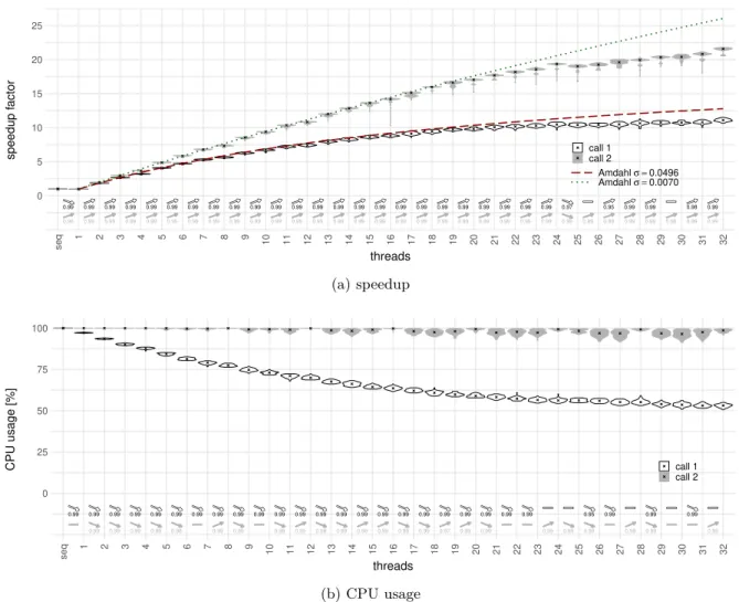
Many papers present scalability curves which cannot be well described by Amdahl’s law. A superlinear speedup is reported in [9] for dense matrix multiplication. That is a scaling behavior better than linear with the number of used cores, so better than Amdahl’s law with σ = 0. The same authors give reasons for such behavior in [10]. Non-persistent algorithms finish when one thread found a solution and thus might finish in less total instructions when run in parallel mode. Persistent algorithms (like matrix multiplication) can show constructive data sharing in shared caches. One core might implicitly prefetch data from memory for another core. The most common case they identify is an increased amount of available cache capacity when using more cores. Private caches of cores can only be used when executing on all cores in parallel, thus we do not only add computing power but also increase the total cache capacity when increasing the number of used cores. This is especially important for architectures with large private caches, like the Skylake processors we use: Intel increased the private L2 cache to 1 MiB from only 256 KiB in previous generations.

Didier et al. include a speedup curve which decreases with increasing thread count after a certain maximum [11], whereby they always use less or the same amount of threads as physical cores available. This is predicted by their timing model as well as occurring in their measurements. They argue that this happens due to memory access interference, where all accesses together saturate the available memory bandwidth. We come back to this explanation after presenting our results in the conclusion.

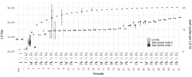
The performance evaluation of the Skylake architecture in [12] also contains measurements for matrix multiplication. Again the thread count is always smaller or equal to the core count. Their curve

(13)

contains steps, i.e. flat regions and increases only at certain thread counts, similar to what we observe in our data in Figure 5a (page 26). On the steps, performance sometimes even decreases for increasing thread count. The authors attribute all this behavior, especially the end of scaling after 16 used cores, to thermal throttling of the chip. After our experiments, we will see that this is only part of the cause. Even the extensions to Amdahl’s law shown in Section 2.2 cannot explain any of those behaviors well. Most of the speedup curves in the literature are not well analyzed and no or only a simple interpretation is provided. This motivates our work.

2.4 Interference analysis for real-time systems

Nowadays, even in the community of real-time systems, multicores are more and more used in order to meet increasing performance requirements. Safe upper bounds on the Worst Case Execution Time (WCET) are needed here, thus researchers started to study how cores interfere with each other through shared resources in multicore systems.

Wilhelm et al. give a first static timing analysis of caches and buses in [13]. They highlight issues in the timing analysis due to sharing of those resources in multicores. For example, to gain information on shared cache states all possible interleavings of accesses from the different cores need to be considered. As a consequence, the authors instead recommend to try to eliminate interferences on shared resources as much as possible in the hardware architecture design. In our context of HPC, this is obviously infeasible as e.g. shared caches are crucial for performance. Furthermore, Wilhelm et al. discuss that modern architectures are pipelined with complex features (e.g. out-of-order execution). They might thus exhibit timing anomalies as presented in [14] and formally defined in [15]. Simplified, those are situations where a local worst case does not cause the global worst case of execution time, e.g. a cache miss might in the end result in a shorter runtime compared to a hit due to following decisions of other processor features. Based on this, Wilhelm et al. [13] classify architectures as fully timing compositional (no timing anomalies), compositional with constant-bounded effects (timing anomaly effects can be bounded with a fixed number of penalty cycles) and noncompositional architectures (timing anomalies can have arbitrary effects). Most proposed static analysis for resource sharing architectures in the literature (e.g. [16] and [17]) are only feasible for (fully) compositional architectures. Penalties of individual effects can be viewed in isolation and then added together in this case. Otherwise, all effects have to be viewed together which results in exploding complexity. Hahn et al. [18] provide a clearer notion of this property. However, the Intel Skylake processor (x86-64) we use in this work has to be assumed noncompositional. In addition, many internals of the processors are secrets of Intel so that we cannot model them for a detailed timing analysis. Nonetheless, we can still derive an approximate parallel scaling behavior similar to the models of Section 2.2.

Measurement based approaches aiming to quantify interference through experiments complement the static analyses. In order to obtain the worst-case interference, Radojković et al. [19] use resource stressing benchmarks, i.e. they run a test code that makes extensive use of a specific shared resource. This might be very pessimistic as a real co-running application would stress the resources less. Further-more, it might not be clear what is the worst-case interference for a noncompositional architecture, due to complex interactions. It might rarely occur in measurements. Also, as we see in our experimental data, only multiple cores together might be able to stress a shared resource fully.

A general overview over resource sharing is provided in [1]. The authors group shared resources into bandwidth resources (e.g. shared buses) and storage resources (e.g. shared cache capacity). Resources might be shared between all cores in the system, at chip level or even just between pairs of cores. We use this classification as a basis in this work.

2.5 Scheduling for multicore processors

Resource sharing and especially contention of resources has been studied in the context of co-scheduling, where a workload composed of multiple applications needs to be scheduled over time and on the set of

(14)

available cores of a system.

Antonopoulos et al. [20] observe that the memory bandwidth often limits performance for (bus-based) computing systems. They propose co-scheduling policies which measure the memory bus band-width usage of applications and select co-runners such that they use as much of the available bandband-width as possible in each scheduling quantum, but do not exceed its limit.

In [21], Knauerhase et al. focus on balancing the load between multiple Last Level Caches (LLCs). The researchers argue that the number of cache misses per cycle indicate cache interferences well, thus they use it as heuristic to guide their co-scheduling decisions.

Zhuravlev et al. [22] make a more detailed analysis of the impact of various shared resources when two applications run together - they study the DRAM controller, the Front Side Bus (FSB), the LLC and resources involved in prefetching (which also includes the memory controller and the FSB). Based on this, they discuss schemes to predict mutual degradation of co-running applications, including sophisticated strategies based on cache access patterns. The authors conclude that simply the number of LLC misses per cycle, as previously used by Knauerhase et al., serve as a good heuristic to estimate the degree of contention, because the misses highly correlate with DRAM, FSB and prefetch requests. The motivation for the heuristic thus differs from [21], where LLC contention is the optimization target. The work of Bhadauria and McKee [23] considers multithreaded programs, their scheduler in ad-dition decides on the number of threads to use for each application. In their solution, an application which does not scale well to high thread counts because it saturates a hardware resource can run with a lower thread count and another application with lower intensity on this resource is co-scheduled on the remaining cores. As heuristic to predict shared resource contention, they also use the LLC miss rate, and the occupancy of the (shared) data bus between processor chips in their target system.

Sasaki et al. [24] follow a similar approach but base their scheduling decisions only on the scalability of the programs when run in isolation, instead of the contention for resources caused by the possible schedules.

In [25] the authors consider modern NUMA machines where each processor chip manages part of the memory, instead a single memory accessed over a shared bus. Four factors are identified to be important: contention either for the LLC, memory controller or interconnect, as well as the latency of remote memory accesses. The previous solutions are found to not work well in such a situation because they frequently change the core on which a thread runs but the data stays in memory at the original node. This increases interconnect contention, contention for the memory controller at the remote node and introduces remote memory access latency. Only LLC contention is reduced by the co-scheduling algorithm on such a hardware architecture. The authors thus propose a new algorithm, which moves threads only when clearly beneficial and also migrates a certain amount of actively used memory pages with the thread to the new node. The load on the memory controller is better balanced and the chip interconnect has to handle only a few remote memory accesses.

In addition, works targeting Simultaneous Multithreading (SMT) processors exist, for example [26, 27, 28]. Those also try to maximize the symbiosis between co-running threads, but at the level of an individual physical core instead of at chip level. The aim is again to achieve a high, yet not overloading, usage of shared hardware resources.

Scalability of a parallel application, which is the topic of this work, can be seen as a special case of co-scheduling where all threads have identical characteristics. The threads of a single multithreaded application can in addition share memory regions, which allows for constructive cache sharing in this case. Still, similar microarchitectural resources will present bottlenecks and insights can be used in both disciplines.

The next section introduces our experiments and provides all details required to understand and reproduce our results shown afterwards in Section 4.

(15)

3 Experiment setup

Performance measurements highly depend on many details of the experiment design as well as the used hardware and software configuration. We thus detail here the most important parameters of our data collection environment needed to understand the obtained scalability curves in Section 4. We provide many additional details to allow reproduction of the results. As [29] shows, additional hidden factors might influence performance and add bias to our measurements. However, we are confident that the general conclusions are valid and can be recreated with the given information.

We repeat all our measurements N times with identical parameters to capture variations which can be significant for parallel (OpenMP) applications as shown by Mazouz et al. [30], we use N = 50 executions. Our obtained data is thus not a single value but multiple observations of random variables of which we report the complete distributions instead of aggregating them into a single value like median or mean.

In this section, we first define important terms. Then, we describe the used hardware and software environment. The last part treats our methodology including the used test applications, parallel and sequential program versions, NUMA considerations and gives details on our way of measuring.

3.1 Definitions of used metrics and scalability

Let us first define some terms important for this work, to avoid any ambiguity.

Experiment execution With an experiment execution we mean a specific instance of running an

application. In the context of this work, we can uniquely identify such an execution by the application

A, the used thread count p ∈ N∗_{and the index of the measurement repetition n ∈ {0, 1, ..., N −1} =: I,}

so by the tuple E = (A, p, n). The application A in here includes the actual executed binary code as well as the runtime configuration (in particular OpenMP parameters), except for the used thread count

pwhich we denote explicitly to ease the definition of our metrics. We call the set of all applications K. Runtime Each of our application contains multiple timed sections, in particular multiple calls of the

benchmark function which Section 3.4.5 details further. Those timed sections are denoted by s ∈ N0.

For one timed section s of an experiment execution E = (A, p, n), we distinguish three different times: • treal(A, p, n, s) is the real time, i.e. the wall clock time, needed for the timed part of the

applica-tion. We also refer to this as runtime. • ti

user(A, p, n, s) denotes the time which thread i of our application spent in user mode

• ti

sys(A, p, n, s) means the time that thread i was running in system (kernel) mode

Speedup For each application, we also generate a corresponding purely sequential version. It serves

as a baseline, i.e. we use it as a reference for the parallel versions. We detail this further in Section 3.4.3. All speedups presented in this work are the speedup in the real time between a specific experiment execution E = (A, p, n) and the median runtime of all repetitions of this associated sequential program version. Since the sequential versions show small variability [30] and the base runtime only introduces a fixed scaling, using just the median of all sequential executions as a reference is acceptable. Let us denote

Aseq the sequential application belonging to an application A. The function Speedupexecution: K ×

N∗× I × N0→ R then gives the speedup of a timed section s for one specific execution:

Speedupexecution(A, p, n, s) =

median{treal(Aseq,1, i, s) | i ∈ I}

treal(A, p, n, s)

(16)

Similarly, we define the function Speedupempirical: N∗ → RN which returns for a thread count p the

set of speedups obtained in the different repetitions. We consider a fixed application A and a given timed section s, so those two become parameters instead of function variables:

Speedupempirical(p) = {Speedupexecution(A, p, j, s) | j ∈ I}

= {median{treal(Aseq,1, i, s) | i ∈ I}

treal(A, p, j, s) | j ∈ I}

(8)

CPU usage (per thread) The CPU usage is given by a function CP U_usageexecution: K × N∗×

I × N0 → R for one execution. We define it divided by the thread count p to get a metric which is

comparable for different thread counts:

CP U_usageexecution(A, p, n, s) = p−1

P

i=0

(ti

user(A, p, n, s) + tisys(A, p, n, s))

p × treal(A, p, n, s) (9)

This is a value between 0 % and 100 %. For our experiments, the system time is small and negligible. Note that e.g. the top command in Linux uses a different notion and reports a total CPU usage which is not divided by the thread count, so a value between 0 % and p × 100 % instead.

This metric allows us to monitor the fraction of the execution time during which the cores used by our application are actually doing computations, as seen by the OS and reported to users. Low values indicate that part of the cores are idle at some point during the application execution, e.g. because of a sequential program part or because they are waiting for another core to finish (synchronization). We show that the effects we study in this work are hidden from the OS, i.e. the reported CPU usage is high even though the cores actually spend a large amount of time waiting (stalling).

Analogous to the speedup in Equation (8), let us define a function CP U_usageempirical: N∗→ RN

returning the set of all values for all repetitions of the same application A in a given timed section s:

CP U_usageempirical(p) = {CP U_usageexecution(A, p, j, s) | j ∈ I}

= {

p−1

P

i=0

(ti

user(A, p, j, s) + tisys(A, p, j, s))

p × treal(A, p, j, s)

| j ∈ I}

(10)

Scalability Under scalability we understand the behavior of the application and our machine when

increasing the exploitation of coarse-grained data parallelism, i.e. increasing the number of parallel executed threads on the fixed hardware architecture. In particular, we mean the speedup of runtime while keeping the workload constant as in Amdahl’s analysis (strong scaling, see Section 2.1) opposed to work size scaling proposed by Gustafson (weak scaling) [31]. We scale a single (OpenMP) application, with each parallel thread executing exactly the same code with the same properties (type of used instructions, cache usage, ...). This is very different from scalability of task level parallelism, e.g. of a web server for more users which might execute different tasks at the same time.

3.2 Machine description

The machine we use for all our experiments is a Dell Precision 7920 workstation. Figure 2 gives a simplified view on the characteristics of its architecture. It is equipped with an Intel Xeon Gold 6130 multicore processor in each of its two sockets. Each of those chips contains 16 physical cores, or 32 logical cores with Intel’s SMT technology called Hyper-Threading. The whole machine thus has 32 physical or 64 logical cores. For a precise definition of all terms related to processors, as we use them in this document, please also have a look at the Glossary (page 54). The cores support AVX-512

(17)

c c c c c c c c c c c c c c c c IMC IMC L3 -22 MiB CPU chip 0 DRAM - 16 GiB DRAM - 16 GiB DDR4 buses NUMA node 0 c c c c c c c c c c c c c c c c IMC IMC L3 -22 MiB CPU ch ip 1 DRAM - 16 GiB DRAM - 16 GiB DDR4 buses NUMA node 1 UPI

links _{core main} AVX-512

AVX-512 L1 instr.

32 KiB L1 data32 KiB L2 (unied)

1 MiB single core

Figure 2: Architecture of the test machine

SIMD instructions for which they include two vector execution units. They have private L1 caches for instructions and data (32 KiB each), also private L2 caches (1 MiB, unified, inclusive) and a non-inclusive L3 cache shared between all cores of the chip (22 MiB, unified). Table 1 summarizes the most important properties of this cache hierarchy.

Two Integrated Memory Controllers (IMCs) per CPU chip offer three DDR4-DRAM channels each, so 12 channels in total. In our machine, only a single 16 GiB module (running at 2666 MT/s1_{) is}

connected to each IMC, leading to 64 GiB of total memory. A DDR4 bus is 64 bit wide, hence transmits 8 bytes in each transfer. All the four buses together in parallel thus result in a theoretical available peak memory bandwidth of 4 × 2666 MT/s1_×_{8 bytes/T}1_{= 85.33 GB/s for our machine. The two chips are}

connected over two cache-coherent Intel Ultra Path Interconnect (UPI) links. Each CPU chip together with the RAM connected to it, however, forms a Non-Uniform Memory Access (NUMA) node. That implies that accesses to memory locations physically located in memory at the other node are slower than accesses to local memory locations.

The CPUs use a base frequency of 2.1 GHz. Our aim is to generate reproducible results. We thus deactivate the Dynamic Voltage and Frequency Scaling (DVFS) features of the processors in our experiments as far as possible. Since those mechanisms still have an impact on our experiment results, the next section describes them as far as required to follow our argumentation during the data analysis.

1_T_{denotes data transfer operations on a communication bus. For a bus using Double Data Rate (DDR), two transfers} occur per clock cycle - one on the rising and one on the falling edge of the clock signal. The amount of data transmitted per transfer is equal to the bus width. 1 MT = 106_T.

Table 1: Cache hierarchy of the Skylake architecture [32]

Line Latency

Content Size Topology Inclusion Associativity size (cycles)

L1 instr. instructions 32 KiB private - 8-way 64 B

L1 data data 32 KiB private - 8-way 64 B 4-5

L2 unified 1 MiB private inclusive 16-way 64 B 14 L3 unified 1.375 MiB/core shared non-inclusive 11-way 64 B 50-70

(18)

3.2.1 DVFS in Intel processors

Intel uses complex DVFS mechanisms in their modern processors to limit power consumption and keep the heat dissipation in a reasonable range. Sleep states (C-states) allow idle cores to consume less power by turning off parts of the cores, generally the deeper the sleep state is the less power is consumed but the longer is the wake-up time. The OS controls these and explicitly requests the desired C-state. When a core is in running mode, so in C0 state, it can use different P-states (performance states), mapping to different operating frequencies and voltages. Those thus offer various performance levels at corresponding power consumptions. Under normal conditions, e.g. a cooling system as the specified Thermal Design Power (TDP) of the chip, the CPU should be able to maintain all these frequencies steadily on all cores. Turbo Boost (2.0) extends the performance levels above the nominal (rated) clock frequency. The CPU might not be able to keep those frequencies over a long time and the concretely achievable frequency depends on the actual conditions, often referred to as dynamic overclocking.

The most important of those conditions are power consumption and temperature. Latter is measured constantly and in case the chip or individual cores get too warm lower frequencies are selected. Power drawn by the chip should never be larger than what the power supply can provide. For short times (peaks) a relatively high consumption might be acceptable, Intel calls this power limit 3 (PL3). Steadily the supply can provide a bit less power which imposes the next limit (PL2). In the long term, no more power than the cooling system can handle should be consumed (PL1), to prevent running into the overheating case. The power consumption is thus monitored and core frequencies are also throttled if any of these limits is exceeded [33]. In order to not always run into those dynamic limits, the maximum frequency is also limited by two static and deterministic factors: the type of the executed workload and the number of active cores. Here, the type of workload simply means whether or not vector instructions are used and with which vector width. Intel calls those modes license levels and the cores determine their level by the actual density of the different vector instructions (none, AVX2, AVX-512) in the instruction stream, i.e. a single AVX-512 instruction will not cause the highest level. Also, some simple instructions (e.g. shuffle) might belong to a lower level than the more complex ones (e.g. Fused Multiply Add (FMA)). Table 2 gives the allowed maximum frequencies for the CPU in our machine. Base here indicates the guaranteed long term frequency. The number of active cores is determined by cores being either in C0 or in C1/C1E state [34]. Just cores in higher sleep states are considered idle. Only the license mode of each individual core matters for its own maximum frequency, i.e. also if 15 cores run none vector code, the 16th_{core is limited to 1.9 GHz if it uses AVX-512. On the other hand, if 15 cores}

run an AVX-512 load and the last core uses no vector instructions, it can clock up to 2.8 GHz. In many cases the advantage of the larger vector width of AVX-512 vanishes, as a consequence of the lower allowed frequencies due to higher power consumption. In addition, directly following code not using vector instructions anymore can be slowed down as Gottschlag and Bellosa show in [37]. This is likely the reason why compilers use AVX-512 instructions conservatively and only when explicitly told to do so through compiler flags - we come back to this in Section 3.4.2.

The importance of dynamic throttling and static frequency limits varies depending on the processor model. A low power laptop processor (low TDP) will frequently suffer dynamic throttling whereas for a (well cooled) server or workstation processor, like in our experiments, the static limits are sufficient in most cases. We verified that the actual temperature during our benchmarks is far below critical values in all cases, such that no dynamic throttling occurs and the frequency behavior is predictable.

Table 2: Maximum clock frequencies in MHz of the Xeon Gold 6130 [35, 36]

License Active cores

level Instructions Base 1 2 3 4 5 6 7 8 9 10 11 12 13 14 15 16

0 non vector 2100 3700 3500 3400 3100 2800 1 AVX2 1700 3600 3400 3100 2600 2400 2 AVX-512 1300 3500 3100 2400 2100 1900

(19)

Historically, P-states were managed by the OS and frequencies in the Turbo Boost range were automatically used by the hardware when the highest (non-turbo) P-state was chosen. In recent processors, including the here used Skylake chip, Intel completely moved the control over P-states to the hardware with the Speed Shift technology (Hardware Managed P-states, HWP). The OS can however still provide an allowed range of states, now also explicitly including the turbo states. The presented overview is simplified and additional mechanisms, as package level C-states, complement the described ones.

As mentioned we deactivate DVFS through Turbo Boost and P-states in our experiments to generate reproducible results. Please note that the cores might still adapt their clock frequencies under certain conditions as we see later in our results. On the other hand, we directly allow C-states during the experiments as (used) cores should not enter any sleep state in our high load experiments anyway and this configuration is closer to an usual scenario. We discuss the impact of this choice in Section 4.2.5.

3.3 Software environment

Our experiment applications run under a Linux Mint 19 (Tara) OS, with Linux kernel 4.15.0. To reduce interference from other processes during our measurements, we boot the OS in a custom systemd target which minimizes the load on the (idle) system. Only a minimum set of required services as well as SSH are running in this mode. Especially, no graphical environment is started.

We use GCC 8.2.0, ICC 19.0.0.117 and Clang/LLVM 7.0.1 to compile our C++ test codes. Appli-cations using OpenMP link the default OpenMP runtimes in the same versions as the compilers - for GCC to libgomp, for ICC and Clang to libiomp5 respectively libomp5, which use the same source for the implementations. Experiments with Intel’s MKL use it in version 2019.0.0.

3.4 Methodology

As explained, we repeat each measurement N times and thus obtain distributions of random variables for our metrics of interest instead of just a single value. Whenever we claim a difference between two settings, we checked this statistically with the methods provided in [38]. Nonetheless, we employ several methods to reduce variability to a minimum. These include minimal background services, explicitly binding threads to physical cores, as well as controlling NUMA memory allocation. The following sections detail those further, but first we introduce the applications we use for our experiments.

3.4.1 Test applications

The applications we measure in our experiments perform one of the most common and basic examples for parallel computing: matrix multiplication. This problem is a well studied benchmark in HPC. It concentrates in a small kernel many code performance optimization problems and hardware-software interaction phenomena, including instruction scheduling, register allocation, vectorization, loop nest transformation for cache optimization and loop parallelization. Finding the best of all these possible transformations still remains a challenging problem. This single application is thus versatile in itself, i.e. it can show many different microarchitectural behaviors, depending on the actual used machine code implementation. The task is further embarrassingly parallel, i.e. it can be easily decomposed into parallel tasks which are independent of each other and thus do not require any synchronization or communication. This is done by computing a subblock of the overall result matrix in each task. Just one implicit synchronization at the end of the operation is present, as the whole multiplication is only finished when all independent subtasks are completed (persistent algorithm). Thus, the overall runtime is determined by the last finishing task. Consequently, the algorithm is expected to scale very well with increasing parallel execution capabilities.

(20)

We analyze three different implementations to compute MC= βMA× MB+ γMC where MA, MB

and MC are matrices of sizes DN × DP, DP × DM and DN × DM. β and γ are scalars. Our first

two implementations only take care of the special case where β = γ = 1 but can easily be generalized, however, this does not add value to our scalability measurements so that we decided to keep the code as simple as possible. In all experiments we use as matrix sizes DN = DM = 4096 and DP = 3072 to

get sufficiently large matrices but still allow the execution of all our experiments in a reasonable time. The data type of individual matrix elements is either float (4 bytes in memory) or double (8 bytes), depending on the experiment. Consequently, for float the matrices MA and MB occupy 48 MiB of

memory and MC has a size of 64 MiB. In the case of double, the matrices are twice as large so 96 MiB,

respectively 128 MiB. Please note that with these sizes the matrices cannot be fully present in the cache hierarchy of our test machine. We now describe each of the the three implementations in detail.

a) Simple The simple implementation is a straightforward code with three nested loops as shown in

Listing 1. Only the order of the loops - which are interchangeable - is optimized so that accesses to the matrix data follow cache lines and have the best possible data locality behavior for the matrices which are stored in row-major order.

Listing 1: Simple matrix multiplication implementation

1 for (int i = 0; i < D_N; i++) {

2 for (int k = 0; k < D_P; k++) {

3 for (int j = 0; j < D_M; j++) { //AVX-512 vectorized

4 M_C[i][j] += M_A[i][k] * M_B[k][j];

5 } } }

b) Tiling The code of the tiling implementation, presented in Listing 2, explicitly implements tiling

on all three loops using additional loops in the nest. This improves data locality and thus makes efficient use of the processor’s caches. An additional loop at the innermost level (line 9), which gets unrolled, helps the compiler to further reduce data access times by re-using values in processor registers. It is basically another level of tiling on the k-loop. The block sizes, as defined by the code listing, are BSf loat k = 32, BS f loat i = 32, BS f loat j = 1024 and BS f loat

k_reg = 4 for float and BSkdouble = 16, BSdouble

i = 16, BSjdouble = 512 and BSkdouble_reg = 4 for double. Those values were chosen such that the

data accessed by the different loop levels fits well the sizes of the different cache levels of our machine. We provide a detailed justification in Appendix A.

Listing 2: Tiling matrix multiplication implementation

1 for (int i0 = 0; i0 < D_N; i0 += BS_i) {

2 for (int k0 = 0; k0 < D_P; k0 += BS_k) {

3 for (int j0 = 0; j0 < D_M; j0 += BS_j) {

4

5 for (int k2 = k0; k2 < k0 + BS_k; k2 += BS_k_reg) {

6 for (int i = i0; i < i0 + BS_i; i++) {

7 for (int j = j0; j < j0 + BS_j; j++) { //AVX-512 vectorized

8

9 for (int k = k2; k < k2 + BS_k_reg; k++) { //re-use register data

10 M_C[i][j] += M_A[i][k] * M_B[k][j];

11 }

12 } } }

13 } } }

c) MKL Our Math Kernel Library (MKL) version uses the library from Intel to do the computation

(21)

using double as data type. The actual implementation is therefore a secret of Intel and not public. However, we reverse-engineered some parts of it needed to explain our observations.

3.4.2 Compilation details

To compile our implementations, we use three different compilers: GCC, ICC and Clang. We pass the options -O3 -std=c++17 -march=skylake-avx512 in all cases. This allows the compilers to use features specific to the Skylake microarchitecture of the processors in our test machine, especially it allows the compilers to use AVX-512 vector instructions. It also enables the highest optimization level composed of a set of optimizations. For all compilers, these include the loop transformations of automatic vectorization and unrolling which are relevant for our benchmarks. ICC also enables loop blocking and indeed applies it for our simple implementation. Note that also GCC and Clang pro-vide similar functionality through their (experimental) polyhedral frameworks Graphite and Polly, however they have to be enabled explicitly.

All our experiment implementation were successfully SIMD vectorized by all three compilers. In all cases vectorization is applied to the innermost loop after unrolling, i.e. in the j-loop. Even though by specifying the CPU microarchitecture we enabled AVX-512 instructions, GCC and ICC are conservative with using the maximum vector width of 512 bits and fall back to 256 bits wide vectors instead. The rationale for this is that AVX-512 instructions are in many cases not worth to use and smaller vectors lead to better performance, especially because the processor is allowed lower maximum frequencies when using the full vector width, in order to limit power consumption and heat dissipation (see Section 3.2.1). For our matrix multiplication example, however, we want to make use of AVX-512. We thus force 512 bit vectors for GCC (-mprefer-vector-width=512) and ICC (-qopt-zmm-usage=high), Clang by default uses the full vector width. This allows each core to do 32 float FMAs or 16 double FMAs in parallel on their two AVX execution units introduced in Section 3.2, leading to high computation throughput but also the demand for fast data fetching. The arrays containing the matrix data are aligned to 64 bytes (512 bit) for aligned accesses by the vector instructions and best caching behavior, one cache line is also 64 bytes on our machine.

In addition, we add the -ffast-math flag for GCC and Clang which allows floating point calcu-lations which are not compliant to the IEEE Standard for Floating-Point Arithmetic (IEEE 754) and might cause changes in the results, e.g. by changing the associativity of a floating point multiplication. ICC already allows similar optimizations with the -O3 flag. Obviously, for experiments with OpenMP, the -fopenmp flag is also necessary. The linker is always instructed to link only the required libraries for each experiment (of OpenMP, MKL, PAPI).

3.4.3 Parallel and sequential versions, thread mapping

We create parallel and sequential versions of our codes. The parallel version makes use of (coarse-grained) data parallelism through OpenMP with a certain number of threads that we vary between measurements. In all our experiments, this thread count is smaller or equal to the number of physical cores in the system. For our two loop based implementations (simple and tiling), we always distribute the iterations of the outermost loop among the threads. In contrary, the sequential version runs in a single thread, i.e. it only uses a single CPU core. We do not link OpenMP in this case to avoid any overhead (compare Figure 1b vs. Figure 1a). However, note that fine-grained data-level parallelism is still used through SIMD execution (AVX-512) also in this version. It serves as a baseline case to which we relate reported speedups. MKL also provides sequential and parallel library versions to which we link our binaries accordingly.

Controlling thread affinity, i.e. binding threads to specific cores for execution, is crucial to reduce variability in program execution times [39]. Without fixing the affinity, the OS kernel is free to choose any mapping of threads to cores and, even worse, migrate threads from one core to another during execution. As some mappings might be superior in terms of performance compared to others, these

(22)

two phenomena lead to differences in runtimes. The kernels decisions depend on many internal factors, the influence is thus random from our point of view and we observe it as variability in the data.

The OpenMP specification since version 4.0 includes thread affinity control. We only present a simplified overview of the mechanisms. For more details, please refer to the specification [40]. In OpenMP terminology, a place defines a location to which threads can be mapped. It is a set of processors, in particular in our context a set of logical CPU cores as seen by the OS. The place list is the list of all the existing places. It is ordered, thus we can identify each place uniquely by its position in the list. Let us call the (i + 1)-th place in this list placei.

In our experiments, we tell OpenMP to create one place per physical core in the place list. This means that each place contains all the logical cores associated with one physical core. The place list is ordered by NUMA nodes, i.e. it includes first all places of NUMA node 0, followed by the places of node 1, and so on. Logical cores are also enumerated, so we can represent them by their numbers. Consider a machine with m physical cores with each two logical cores as ours (2-way SMT). The numbers of all first logical cores are again grouped by NUMA nodes. Furthermore, the two logical cores mapping to the same physical core are the logical core i and the logical core i + m, for i ∈ {0, 1, ..., m − 1}. The

i-th place in this setting is then given by a set of two (logical) core numbers:

placei= {i, i + m} for i ∈ {0, 1, ..., m − 1} (11)

As example we obtain place3 = {3, 35} for our machine, meaning that the fourth place in the place

list contains the logical cores 3 and 35, both mapping to the same physical core. Since parallel regions might be nested in an OpenMP program, not all places of the place list might be available for use in a parallel region, but only a subset which is termed a place partition. However, in our test applications the place partition is identical to the place list.

A policy then defines how the threads are actually mapped to the available places in the place partition:

• The master policy assigns each thread to the same place as the master thread reaching the parallel region, which in our applications is always mapped to place0.

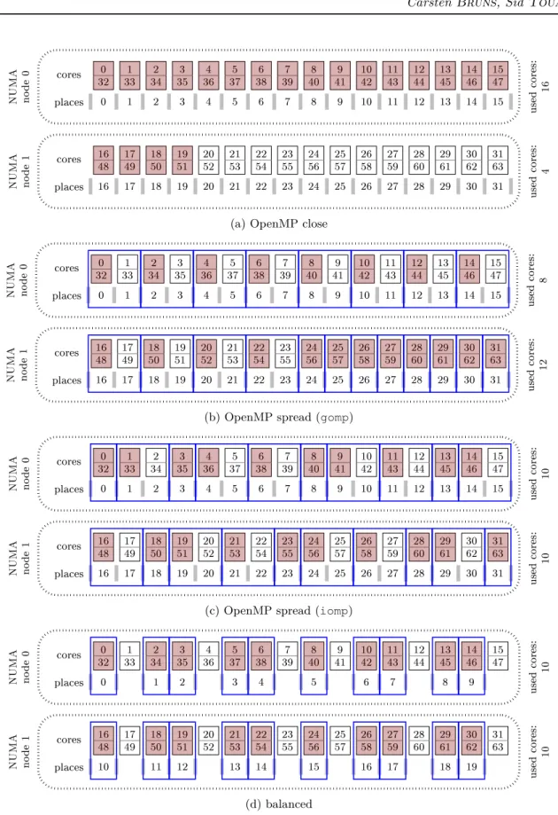
• With close, threads are bound to adjacent places, starting at the encountering master thread. Figure 3a illustrates this policy for our machine with m = 32 physical cores when mapping p = 20 threads. Places available in the place partition are indicated below the cores and used cores are highlighted (filled, red).

• The spread policy in contrary aims to create a sparse distribution of the threads among the available places. Therefore, the place partition list is divided into smaller lists of adjacent places. Every place is included in exactly one of those subsets, which are called subpartitions. The number of subpartitions created is equal to the number of threads to be mapped. Then, one thread is assigned to the first place of each subpartition. When as above m places are available in the place partition list and p threads are to be mapped, for p ≤ m naturally each of those subpartitions will contain either bm/pc or dm/pe places, so their length might differ by one place. However, the specification lets open which of the subpartitions should be the smaller ones and which should be the bigger ones.

The OpenMP runtime of GCC (gomp) implements the spread policy in the simplest way possible: it first places the bigger subpartitions and then the smaller ones. We show this behavior in Figure 3b, where we also indicate the generated subpartitions with solid (blue) borders.

We can see that this is problematic in a NUMA system like ours, where cores are physically located on different NUMA nodes. In such a case, gomp’s strategy of partitioning might lead to an imbalance between the nodes. For our example of Figure 3b, gomp’s implementation leads to 8 threads assigned to cores on node 0 and 12 threads to node 1, so a strong imbalance. More general, if p =m

2 both nodes

(23)

0 32 331 342 353 364 375 386 397 408 419 1042 1143 1244 1345 1446 1547 0 1 2 3 4 5 6 7 8 9 10 11 12 13 14 15 cores places NUMA node 0 used cores: 16 16 48 1749 1850 1951 2052 2153 2254 2355 2456 2557 2658 2759 2860 2961 3062 3163 16 17 18 19 20 21 22 23 24 25 26 27 28 29 30 31 cores places NUMA node 1 used cores: 4

(a) OpenMP close

(b) OpenMP spread (gomp)

(c) OpenMP spread (iomp)

0 32 331 342 353 364 375 386 397 408 419 1042 1143 1244 1345 1446 1547 0 1 2 3 4 5 6 7 8 9 cores places NUMA node 0 used cores: 10 16 48 1749 1850 1951 2052 2153 2254 2355 2456 2557 2658 2759 2860 2961 3062 3163 10 11 12 13 14 15 16 17 18 19 cores places NUMA node 1 used cores: 10 (d) balanced

(24)

threads will always be added on node 1 until all its cores are used: partitions will have either length two or one and gomp first creates all subpartitions of size two.

The OpenMP runtime of ICC/Clang implements a more sophisticated partitioning scheme that assigns the same amount of threads to all NUMA nodes, except for one thread difference for odd thread counts. We see how this improves the situation in our example case in Figure 3c. Thus, we also implemented an affinity mapping scheme that assures the property of balance between NUMA nodes. To keep the implementation simple, we solely change the place partition. We provide to the OpenMP runtime a list containing one place for each physical core which we want to use for one of the p threads, instead of all cores present in the system as before. Since we give only exactly as many places as threads in our application, this results in a fixed mapping, independent of the spread or close policy of OpenMP- both will map one thread to each of the places. Let nint: R → Z be the function that returns the nearest integer to its input, with round to the next even integer for ties. Each place contains again the two logical cores of one physical core, however, this time we define:

placei= {nint(i ×

m

p), nint(i × m

p) + m} for i ∈ {0, 1, ..., p − 1} (12)

This spreads the threads by maximizing the distance between the used core numbers, but as desired still ensures balance between NUMA nodes, as we clearly see in Figure 3d. We thus refer to this policy as balanced in this report.

In the literature, more complex affinity mapping schemes are studied (e.g. [41, 42]). Those are out of scope for this work, as we only want to remove thread mapping variability and obtain a balanced NUMA load distribution. Our balanced mapping is sufficient for these aims. The sequential version also forces the Linux scheduler to always run it on the same core (core 0) through the sched_setaffinity system call.

Note that we let Hyper-Threading activated but always just assign a single thread of our application to each physical core. This allows the OS to schedule other processes on logical cores mapping to a physical core used by our application but is only relevant when we use (almost) all physical cores.

3.4.4 NUMA memory allocation

Our test machine has two NUMA nodes as shown in Figure 2. Data in the main memory can thus be physically located in those two different locations. Allocation of memory happens in granularity of memory pages of usually 4 KiB size. By default, the Linux kernel applies the local policy: memory is allocated on the node from which it is first accessed. This is problematic when data initialization happens in a sequential part of the code, since all memory gets allocated on a single node, but the actual computation happens in parallel on multiple nodes [43]. The Linux kernel (since version 3.15) solves this by monitoring accesses and migrating pages to other nodes if judged beneficial by a heuristic. This is also useful when threads are not bound to cores and might be scheduled on different nodes over time. However, it introduces another non-deterministic factor and thus runtime variability, depending on when and how page migrations happen.

To avoid this, we use the bind and interleaved policies. The first allows memory to be allocated only on a subset of nodes and not to migrate afterwards. We only allow node 0 in this case. We also fix the memory allocation for the sequential program version, even though no migrations should happen as every access to the data comes from the same node. The second policy allocates pages in a round-robin fashion to an allowed set of nodes. Here, we allow both NUMA nodes, i.e. new pages are assigned alternating between the two nodes. Note that if we bind all data to a single node only half the memory bandwidth is available compared to the interleaved case.

3.4.5 Measurement method

A shell script controls the repetitions of an experiment instead of running the same function multiple times in the C++ code. This is important to make the executions independent of each other: each

Empirical study of Amdahl’s law on multicore processors

HAL Id: hal-02404346

https://hal.inria.fr/hal-02404346v2

Submitted on 2 Jun 2020

HAL is a multi-disciplinary open access

archive for the deposit and dissemination of

sci-entific research documents, whether they are

pub-lished or not. The documents may come from

teaching and research institutions in France or

L’archive ouverte pluridisciplinaire HAL, est

destinée au dépôt et à la diffusion de documents

scientifiques de niveau recherche, publiés ou non,

émanant des établissements d’enseignement et de

recherche français ou étrangers, des laboratoires

To cite this version:

Carsten Bruns, Sid Touati. Empirical study of Amdahl’s law on multicore processors. [Research

Report] RR-9311, INRIA Sophia-Antipolis Méditerranée; Université Côte d’Azur, CNRS, I3S, France.

2019. �hal-02404346v2�

RESEARCH

REPORT

N° 9311

Amdahl’s law on

multicore processors

Carsten Bruns

, Sid Touati

Contents

1

Introduction

1.1

Runtime of parallel applications

1.2

Contributions

2

State of the art

2.1

Performance of parallel applications and Amdahl’s law

2.2

Extensions to Amdahl’s law

2.3

Reported measurements beyond Amdahl’s law

2.4

Interference analysis for real-time systems

2.5

Scheduling for multicore processors

3

Experiment setup

3.1

Definitions of used metrics and scalability

3.2

Machine description

3.3

Software environment

3.4

Methodology