HAL Id: hal-02640461
https://hal.archives-ouvertes.fr/hal-02640461
Submitted on 28 May 2020HAL is a multi-disciplinary open access archive for the deposit and dissemination of sci-entific research documents, whether they are pub-lished or not. The documents may come from teaching and research institutions in France or abroad, or from public or private research centers.
L’archive ouverte pluridisciplinaire HAL, est destinée au dépôt et à la diffusion de documents scientifiques de niveau recherche, publiés ou non, émanant des établissements d’enseignement et de recherche français ou étrangers, des laboratoires publics ou privés.
A penalization method to treat the interface between a
free-fluid region and a fibrous porous medium
Nicola Luminari, Giuseppe Antonio Zampogna, Christophe Airiau, Alessandro
Bottaro
To cite this version:
Nicola Luminari, Giuseppe Antonio Zampogna, Christophe Airiau, Alessandro Bottaro. A penaliza-tion method to treat the interface between a free-fluid region and a fibrous porous medium. Journal of Porous Media, Begell House, 2019, 22 (9), pp.1095-1107. �10.1615/JPorMedia.2019025928�. �hal-02640461�
OATAO is an open access repository that collects the work of Toulouse
researchers and makes it freely available over the web where possible
Any correspondence concerning this service should be sent
to the repository administrator:
tech-oatao@listes-diff.inp-toulouse.fr
This is an author’s version published in:
http://oatao.univ-toulouse.fr/25695
To cite this version:
Luminari, Nicola
and Zampogna, Giuseppe Antonio
and
Airiau, Christophe
and Bottaro, Alessandro A penalization
method to treat the interface between a free-fluid region and a
fibrous porous medium.
(2019) Journal of Porous Media, 22
(9). 1095-1107. ISSN 1091-028X .
Official URL:
https://doi.org/10.1615/JPorMedia.2019025928
A PENA LIZATION METHOD TO TREAT THE
INTERFACE BETWEEN A FREE-FLUID REGION A ND A
FIBROUS POROUS MEDIUM
Nicola Luminari,
1Giuseppe A. Zampogna,
1Christophe Airiau,
1&
Alessandro Bottaro
2,*
1
IMFT (Institut de Mécanique des Fluides de Toulouse), UMR 5502 CNRS/INPT-UPS,
Université de Toulouse,
2 allée du Pr. Camille Soula, Toulouse, France, F-31400
2
DICCA, Università di Genova, 1 via Montallegro, Genova, Italy, 16145
"Address all correspondenœ to: Alessandro Bottaro, DICCA, Università di Genova, 1 via Montallegro, Genova, Italy, 16145, E-mail: alessandro.bottaro@unige.it
The coupling between the flow through a fi brous porous medium and that in a free-fluid region is studied. The flow
dynamics inside the porous medium are described using the volume averaging method applied to the incompressible Navier-Stokes equations in the laminar regime. The two different flow domains are coupled via a penalization method that consists of varying the porous medium properties (porosity and permeability) continuously across the interface. This approach permits the use of the same set of the equations throughout the whole domain. The averaging method is validated against simulations which Jully account for the presence of cylindrical fibers positioned at the bottom wall of a square driven cavity. Numerical experiments are carried out for two different Reynolds numbers, large enough to ensure that inertia
l effects inside the porous domain are not negligible. Good agreement is found when comparing the two approaches.
KEY WORDS: porous media, apparent permeability, porous interface, cavity flow
1. INTRODUCTION
The problem of a fluid flowing above and through porous media is prototypical of many natural flow systems. Severa! animais present some sort of porous coatings, the most well-known examples being perhaps the denticles of sharks (Dean and Bhushan, 2010) and the feathers of birds (Lilley, 1998). Some of these flows display rich interactions between the porous medium and the exterior flow field, for example in the f01m of v01tex stmctures near the dividing swface (Jimenez et al., 2001). These vortices can modify the energy spectrum of the flow field (Finnigan, 2000), suggesting the use of porous layers as synthetic, passive control devices to delay separation and/or reduce drag (Klausmann and Ruck, 2017; Mimeau et al., 2017; Zampogna et al., 2018).
Although the set of equations for the flow both inside and out.side the porous medium is well established, the problem of the interface condition betv.•een a porous medium and a free fluid is still open. Ehrhardt (2012) has given a concise but ve1y clear introduction to the coupling problem; recent advances are repo1ted by Angot et al. (2017), Lacis and Bagheri (2017), and Zampogna et al. (2018).
Approaches used to handle the interface can be classified into two grnups: the one-domain-approach (ODA) and the two-domain-approach (TDA). In the TDA the whole domain is split into two and boundaiy conditions at the interface have to be specified. Historically, the necessity of such a treatment was mainly due to the difference of order betv.•een the Stokes equation and Darcy's law that renders them incompatible at the interface. The Brinkmann model "adjusts" the order of the porous medium equations so that continuity of velocity and traction vectors can be enforced (cf. Devakar and Ramgopal, 2015; Vema and Gupta, 2018); however, the validity of the viscous con-ection
to the Darcy’s law inside the porous medium has been questioned (Nield, 1991). The TDA was followed by Beavers and Joseph (1967), Mikeli´c and J¨ager (2000), Ochoa-Tapia and Whitaker (1995), and Le Bars and Worster (2006). These works have in common the fact that a certain slip velocity has to be specified at the interface. For example, the Beavers and Joseph (1967) condition to leading order reads:
uβ(x1, Γ+) = √ K11 α ∂uβ(x1, Γ+) ∂x2 ,
where uβis the velocity vector tangential to the dividing surface, whose normal direction is x2. Γ+ represents the
wall-normal coordinate right above the interface, K11is the permeability component in the tangential direction, and
α is a coefficient based on the porous medium structure and geometry. Other formulations change and/or extend this equation, basically maintaining a slip velocity at the interface, function of one or more parameters which can be tuned to fit experimental data.
On the contrary, in the ODA approach the final averaged equations are valid through the whole domain and the quantities that define the presence of the porous media, i.e., the porosity and the inverse of the permeability, vanish in the free-fluid region. This method is also known as penalization method. One of the first applications of the penal-ization method was described by Caltagirone (1994). Later on, it was used by many other authors, including Bruneau and Mortazavi (2004, 2008), Bruneau et al. (2010) and Hussong et al. (2011). The two approaches (TDA and ODA) require at least one parameter to close the formulation. The advantage of using the penalization method is that the parameter needed is the spatial distribution of the porosity field which is easily available on a known medium geom-etry. However, it is still not clear how the permeability in the transition/interface zone should be varied. Most authors propose a sharp jump from the value in the porous medium to that in the free-fluid region. Neglecting the variation of permeability across the transition zone appears to be acceptable, even though examples of linear variation of this term exist (Caltagirone, 1994). Hussong et al. (2011) make a direct comparison with a direct numerical simulations (DNS) simulation which includes a discretization of all the pores and indicates that the variation of permeability is very important in order to have accurate comparison with high-fidelity computations.
A direct comparison between the ODA and the TDA is presented by Cimolin and Discacciati (2013), who con-clude that the macroscopic description of the interface provided by the two different methods is similar. They also point out that the penalization method has the advantage of being easily implemented in a Navier–Stokes solver without convergence problems, unlike the TDA.
There is evidence in the literature (Ochoa-Tapia et al., 2017) that a transition zone the size of the pore scale exists, in which velocity and pressure exhibit a continuous variation rather than a steep one. It has been demonstrated by the same authors that the transition zone is physical and not a result of the averaging procedure.
The present work adopts the penalization approach with the porosity variation computed directly from the ge-ometry of the fibrous medium via a moving average. The effective permeability is varied linearly at the interface with the same law as the porosity. This interface approach coupled with the macroscopic volume-averaged equations is validated against a full microscopic direct numerical simulation. Computations are performed on a closed cavity configuration with a lower porous layer. This represents a more difficult test bed for the porous/fluid coupling than the classical Poiseuille flow, because of the presence of recirculating motion, with both velocity components different from zero at the dividing surface.
2. CLOSED CAVITY PROBLEM DESCRIPTION
The configuration chosen to test our approach is the square cavity of side L, depicted in Fig. 1. The lateral and bottom walls are fixed and a constant velocity Utopis specified at the top side. On the front and back sides (i.e., along x3)
periodic boundary conditions are enforced. The distance between the front and the back side of the cavity is indicated as ℓ. A rigid porous medium made by regularly arranged fibers is set at the bottom of the cavity, of vertical extension equal to h = L/3. The representative elementary volume, REV , of the porous medium is a cubic cell of size ℓ3with a cylinder of diameter d at its center. The cylinders are disposed in a regular arrangement and 50 fibers are assumed to be present in the cavity (i.e., ℓ = 0.02 L).
⟨ψβ⟩ = 1 Vβ+ Vσ ∫ Vβ ψβ(x) dVβ, (2)
and the intrinsic average is
⟨ψβ⟩β= 1 Vβ ∫ Vβ ψβ(x) dVβ. (3)
These operators are related by⟨ψβ⟩ = ϵ⟨ψβ⟩β, and are applied through the whole porous domain using a REV of dimension ℓ3. The centroid of the REV, over which the averaging operations are performed, spans all the porous
domain extension. An example of REV adopted in this case is depicted in Fig. 1, on the right. The choice of the REV size is trivial for ordered porous media, as in our case; however, there are delicate technical issues on the REV choice when the medium is disordered (Davit and Quintard, 2017). As a rule of thumb, the REV is the smallest fluid domain over which periodic boundary conditions can be applied. The averaging procedure yields a two-dimensional averaged field as a result; the only nonzero values are in the x1and x2directions. This is due to the symmetry of velocity and
pressure in the x3direction that returns zero averaged fields.
4. MACROSCOPIC APPROACH: VOLUME-AVERAGED NAVIER-STOKES (VANS) METHOD 4.1 A Brief Description of the Method
A more computationally convenient way to solve the problem is to apply the VANS method to derive a homogenized model for the flow inside the porous medium, described as a continuum.
In order to derive the averaged version of system (1) we first define the fundamental ingredients needed in the development. The first one consists of the averaging operators (2) and (3), introduced above. The second is the decomposition of any flow variableψ into an intrinsic average part⟨ψ⟩βplus a perturbation ˜ψ, as: ψ =⟨ψ⟩β+ ˜ψ. Applying the above decomposition and averaging the first two equations of system (1) we have
∂⟨vβ⟩β ∂t + 1 ε∇ · ( ε⟨vβ⟩β⟨vβ⟩β ) =− 1 ρβ∇⟨p β⟩β+ νβ∇2⟨vβ⟩β+ νβ ε ∇ε · ∇⟨vβ⟩ β +νβ ε ⟨vβ⟩ β∇2 ε + 1 Vβ ∫ Aβσ ( −p˜β ρβ I + νβ∇˜vβ ) · nβσdA, (4) ∇ ·(ε⟨vβ⟩β ) = 0, (5)
upon neglecting in Eq. (4) the sub-REV-scale dispersion term (linked to⟨˜vβ˜vβ⟩β) which is often small in porous media flows (Breugem, 2005; Breugem et al., 2006). The derivation of Eqs. (4) and (5) is rather involved and is presented in details by Whitaker (1996, 1999) and Breugem et al. (2006); it relies on the use of the spatial averaging
theorem (Anderson and Jackson, 1967) to transform the average of a gradient into the gradient of an average, which is
the reason why the integral term in Eq. (4) arises. Such a term represents the drag (per unit mass) due to surface forces at the fluid–solid interface of the medium. It is called the Darcy–Forchheimer microscale force, Fm, and it depends
on perturbation quantities only. The equations are, however, often to be solved at the macroscale, so that a macroscale force model, FM, must be used to replace Fmin the governing equation. Such a model is based on a permeability tensor, K, and a Forchheimer tensor, F, and reads:
FM=−ν
βεK−1(I + F)⟨vβ⟩β=−νβεH−1⟨vβ⟩β,
where H = K−1(I + F) is called the apparent permeability tensor. The system is closed by imposing Fm = FM. One of the main aspects of the VANS approach consists of the identification of the permeability and Forchheimer tensors. Some empirical regressions are available in the literature for simple porous media geometries (Carman, 1937; Kozeny, 1927) in the limit of Stokes flow within the pores. It is however also possible to derive some generalized closure problems for the solution of the two tensors, as discussed by Whitaker (1986, 1996).
∂⟨vβ⟩β ∂t + 1 ε∇ · [ ε⟨vβ⟩β⟨vβ⟩β ] =− 1 ρβ∇⟨p β⟩β+ νβ∇2⟨vβ⟩β+ νβ ε ∇ε · ∇⟨vβ⟩ β +νβ ε ⟨vβ⟩ β∇2ε− ν βεH−1⟨vβ⟩β, ∇ ·(ε⟨vβ⟩β ) = 0, ⟨vβ⟩β= 0 at x1= 0, L and x2 = 0, ⟨vβ⟩β= Utope1 at x2= L. (6)
The boundary conditions are the same as the DNS approach except for the x3dimension that in the present case
disappears through averaging. The solution of system (6) gives directly the averaged velocity and pressure fields to be compared to the averaged DNS fields.
4.2 Treatment of the Interface
In order to use the so-called penalization method, the porosity field and the effective permeability have to be defined in the whole domain, i.e., Ωpand Ωf. In the free fluid the porosity is, of course, unitary and the effective permeability
infinite. With such numerical values the Navier–Stokes system (1) is retrieved from system (6) after some simplifi-cations. In the porous medium far from the interface the porosity is constant and set equal to 0.8. The permeability is also constant and the two independent components of the tensor have been taken from a posteriori evaluations of the homogenized-DNS problem. This requires the inversion of the Darcy system⟨vβ⟩β=−H/(εµβ)∇⟨pβ⟩β. The numerical values for H, given in Table 1, are different at the macroscopic Reynolds numbers of 100 and 1000, an indication of the fact that inertia through the pores is no more negligible. The values in Table 1 are by no means exact: they represent the peak values of the computed distributions.
The apparent permeability tensor H is diagonal; this is consistent with the results of Luminari et al. (2018) for low pore Reynolds number. It turns out that in the cavity the pore Reynolds number, based on the local velocity and the diameter of the fibers, is always below 5 for the cases tested.
The most delicate part is the matching of properties across the dividing surface. The exact profile for the porosity field can be computed knowing the geometry of the medium.
By a moving average procedure it is easily found thatε is equal to:
ε(x2) = 1 x2 > (h + ℓ/2), ε +1− ε ℓ [x2− (h − ℓ/2)] (h − ℓ/2) < x2 < (h + ℓ/2), ε x2 6 (h − ℓ/2), (7)
to within the averaging approximation. A similar relation is used for the inverse of the effective permeability field, with Hiireferring to the effective permeability components of the deep medium, reported in Table 1.
Hii−1(x2) = 0 x2> (h + ℓ/2), Hii−1− Hii−1 ℓ [x2− (h − ℓ/2)] (h − ℓ/2) < x2< (h + ℓ/2), Hii−1 x26 (h − ℓ/2). (8)
TABLE 1: Apparent permeability values from Zampogna
and Bottaro (2016)
Re H11= H22 H33
100 2.63× 10⁻² 5.49× 10⁻² 1000 2.65× 10⁻² 5.63× 10⁻²
The data analysis by Luminari et al. (2018) suggests that the components of H are mostly driven by the porosity, so it is acceptable to assume that the same dependence on x2occurs for both the porosity and the permeability fields.
The analysis in Kozeny (1927) and Ergun and Orning (1949) also shows that, in other porous media geometries, the permeability follows a linear trend with the porosity. For comparison purposes, we have also tested a step variation of the permeability at the dividing surfaces (results not shown), finding significant differences when compared to the direct simulation results. Finally, observe that in Eq. (6) the terms containing the first derivative of the porosity remain as sources in the equations near the interface, whereas the Laplacian ofε disappears.
4.3 The Flow in the Free-Fluid Domain
Before addressing the problem of the fluid-porous dividing surface, it is appropriate to inspect the flow solutions in the free-fluid region, Ωf, as they arise from the three-dimensional simulations in the presence of fibers (upon
averaging along x3), and compare them to corresponding two-dimensional solutions obtained in a driven cavity of
height (2/3)L, bounded by solid walls. Such a comparison, at two values of the Reynolds number, is displayed in Fig. 2 and allows an appreciation of the effects that we wish to capture by the use of the volume-averaged Navier– Stokes equations. An expected large recirculation vortex is observed at the two values of Reynolds number, and larger corner vortices appear when Re = 1000. Since the same values of the streamfunction isolines — computed on the basis of the u and v velocity components — are plotted in each frame of the figure, and given that solid and dashed lines are very close to one another in each frame, it is clear that the porous layer provides a major obstacle to the flowing by the fluid, and acts in a way very similar to a solid, impermeable wall. As we will see later, the fluid permeates the Ωp domain only minimally, and velocity components which are typically three orders of magnitude smaller than in
the pure fluid region are present when 0 < x2≤ h. Thus, the case we are focusing upon does not represent a simple
test case for the penalization method, since very small effects are looked at.
The next section will focus more closely on the porous domain; we aim to demonstrate that the use of the VANS equations coupled to the moving average procedure for ε and Hii represents a valid alternative to the complete
three-dimensional numerical description of the flow over the porous layer and through the pores, at a fraction of the computational cost.
5. CAVITY FLOW AT Re = 100
This section presents the comparison between the microscopic and macroscopic approaches for the cavity at Re = 100. The two different sets of equations are solved using the finite volume method implemented in the OpenFOAM library
FIG. 2: Streamlines in the pure fluid region, Ωf, for the flow in the presence of fibers (continuous lines) and the flow in a domain
(Weller et al., 1998). In the case of the VANS approach a specific solver has been developed to account for all the extra terms present in system (6) as compared to the Navier–Stokes equations. Figures 3 and 4 show the pressure gradient terms and the velocity fields for the two different approaches.
Each field is made non-dimensional using the macroscopic length L and the velocity scale, Utop, as follows:
u∗= u/Utop, v∗= v/Utop,
∂p∗ ∂x1∗ = L ρβUtop2 ∂p ∂x1 , ∂p ∗ ∂x2∗ = L ρβUtop2 ∂p ∂x2 .
At Reynolds number equal to 100 a good agreement is found for both the velocity components and the pressure gradient (Fig. 3). The contours and the location of the local minima and maxima are the same for the two approaches. Focusing on the numerical values, for some fields the relative errors are not negligible; however, the trends are always
FIG. 3: Left: VANS approach. Right: Homogenized DNS approach. The figures show, from top to bottom, the two components of
the pressure gradient and the streamlines inside the porous domain Ωpfor Re = 100.
FIG. 4: View of the macroscopic profile of u∗(left frame) and v∗(right frames) for x1∗ = 0.5 (middle of the cavity) for the
well captured by the volume-averaged approach and the streamlines inside the porous domain are in very good agreement with the DNS result. The horizontal pressure gradient at the interface (Fig. 5) is quite overestimated by the VANS approach whereas the vertical component shows a relatively good agreement. Some differences between the two models have to be expected since in the VANS approach the micro-scale flow behavior is modeled. This means that some of the small-scale features that the DNS is able to retain are lost in the macroscopic approach. However,
FIG. 5: View of the macroscopic profile of u∗, v∗, ∂p∗/∂x1∗, and ∂p∗/∂x2∗, for x2∗= 0.33 (interface position) for the VANS
Fig. 4 shows that the two approaches produce very similar velocity profiles both near the interface and within the domains Ωpand Ωf.
To quantify the error between the two approaches right at the interface, x∗2 itf = 0.33, we define a metric as:
eq = √∫ 1 0 [ qDN S(x∗1, x∗2 itf)− qV AN S(x∗1, x∗2 itf) ]2 d x∗1 √∫ 1 0 [ qDN S(x∗1, x∗2 itf) ]2 d x∗1 , (9)
with q equal to u∗, v∗, ∂p∗/x1∗, and ∂p∗/∂x2∗. The values from Table 2 confirm that the relative errors associated
with the two velocity components are reasonably small and equal to a few percentage points; conversely, the horizontal component of the pressure gradient displays a non-negligible percentage variation, which decreases with the increase of Re. This discrepancy is probably the price to pay for having neglected the terms linked to⟨˜vβ˜vβ⟩β in Eq. (4) and for the approximation made at the interface for H−1. This disadvantage is largely overcome by the savings in computer time and storage when using the VANS equations instead of performing direct numerical simulations. 6. CAVITY FLOW AT Re = 1000
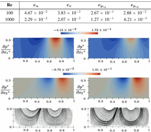
The same comparison has also been carried out for a Reynolds number equal to 1000 and the results within the porous medium are shown in Figs. 6–9. For this case similar conclusions as in the previous case can be made. Both
TABLE 2: Relative L2 error between the VANS and the DNS approaches at the
interface, for the two different Reynolds numbers
Re eu ev ep epx
100 4.67× 10⁻² 3.83× 10⁻² 2.67× 10⁻¹ 2.88× 10⁻² 1000 2.29× 10⁻² 2.07× 10⁻² 1.27× 10⁻¹ 6.21× 10⁻³
FIG. 6: Left: VANS approach. Right: Homogenized DNS approach. The figures show, from top to bottom, the two components of
the pressure gradient and the streamlines inside the porous domain Ωpfor Re = 1000.
FIG. 7: View of the macroscopic profile of u∗, v∗, ∂p∗/∂x1∗, and ∂p∗/∂x2∗, for x2∗= 0.33 (interface position) for the VANS
(red lines with circles) and the DNS approaches (blue lines with crosses) at Re = 1000.
the velocity and the pressure fields display good agreement between the “exact” (DNS) solution and that obtained with the VANS system, both within the porous layer (Fig. 6) and the free-fluid domain (not shown). The velocity at the dividing surface (x2∗= 0.33) is very well described by the volume-averaged resolution of the equations (Fig. 7),
as well as the vertical pressure gradient. The ∂p∗/x1∗term shows the same trend, but the VANS system enhances the
value of the gradient, albeit less than in the lower Re case. This is also borne by the measure reported in Table 2. The vertical velocity distribution through the domain at x1∗ = 0.5 is in excellent agreement between the two approaches
(Fig. 8), and in particular the zooms around the interface demonstrate that the VANS approach is reliable; such plots should be compared to those by Zampogna and Bottaro (2016) from the same configuration, to appreciate even more the accuracy of the volume averaged equation in the form of system (4), (5), as well as the simple choice made for the variation of porosity and permeability across the dividing surface.
FIG. 8: View of the macroscopic profile of u∗(left frame) and v∗(right frames) for x1∗ = 0.5 (middle of the cavity) for the
VANS (red line with circles) and the DNS approaches (blue line with crosses) at Re = 1000.
FIG. 9: Left: VANS approach. Right: Homogenized DNS approach. The figures show the horizontal and the vertical velocity
components in the domain. In all frames the ranges of values plotted have been chosen to highlight the flow structure within the
fibers in the DNS case for Re = 1000.
Focusing on the zone around the porous interface in Fig. 9, the minor differences between the DNS and homoge-nized approach are clear. The DNS shows oscillations in both the vertical and horizontal velocity components due to the presence of the fibers; on the contrary, in the homogenized approach these local oscillations are smoothed out by the averaging operation. However, the oscillations have a very small amplitude and to make them visible the range of values plotted needs to be suitably chosen (see the velocity scales on the right of Fig. 9).
7. CONCLUSIONS
The VANS approach has been used to study the flow field inside a cavity that presents a porous medium at its bottom. A formulation of the penalization method has been proposed for the interface treatment; it is based on the observation that for fibrous media the porosity profile at the interface between the porous region and the free-fluid domain can
be simply computed by a moving average. Knowing the porosity profile we impose the same behavior also for the apparent permeability, since results in Luminari et al. (2018) show the strong link between these two quantities even for varying velocity amplitude and flow angles. This approach simplifies the coupling between the two domains, Ωf
and Ωp, allowing us to use the same set of equations throughout. Both ODA and TDA need at least one free parameter,
for DNS or experimental data to be properly fit. In our case, this degree of freedom is represented by the choice of a linear trend for the components of the apparent permeability.
The proposed approach has been tested in a configuration in which both vertical and horizontal momentum transfer are present. We have also explored two Reynolds numbers for which inertial effect inside the porous medium are not negligible. The two test simulations conducted display promising results. The error metrics are reasonably low for all the measured quantities, with the possible exception of the horizontal pressure gradient which shows differences in the magnitude, but not in the peak positions. Such small differences might also be ascribed to our treatment of the sub-REV-scale dispersion terms. Despite them, we believe that the evidence provided is sufficiently convincing in favor of the averaging approach, which is capable to reproduce the rich dynamics inside porous media at a fraction of the computational cost of a complete DNS.
ACKNOWLEDGMENTS
The authors acknowledge the IDEX Foundation of the University of Toulouse for the financial support granted to the last author under the project “Attractivity Chairs.” The computations have been conducted at the CALMIP center, Grant No. P1540. The OpenFOAM-based VANS solver that has been developed in this study is available at the link: https://github.com/appanacca/porous solvers OF.git.
REFERENCES
Anderson, T. and Jackson, R., A Fluid Mechanical Description of Fluidized Beds, Ind. Eng. Chem. Fundam., vol. 6, pp. 527–538, 1967.
Angot, P., Goyeau, B., and Ochoa-Tapia, J., Asymptotic Modeling of Transport Phenomena at the Interface between a Fluid and a Porous Layer: Jump Conditions, Phys. Rev. E, vol. 95, no. 6, p. 063302, 2017.
Beavers, G. and Joseph, D., Boundary Conditions at a Naturally Permeable Wall, J. Fluid Mech., vol. 30, no. 1, pp. 197–207, 1967. Breugem, W., The Influence of Wall Permeability on Laminar and Turbulent Flows. Theory and Simulations, PhD, Delft University
of Technology, The Netherlands, 2005.
Breugem, W., Boersma, B., and Uittenbogaard, R., The Influence of Wall Permeability on a Turbulent Channel Flow, J. Fluid
Mech., vol. 562, pp. 35–72, 2006.
Bruneau, C., Creus´e, E., Depeyras, D., Gilli´eron, P., and Mortazavi, I., Coupling Active and Passive Techniques to Control the Flow past the Square Back Ahmed Body, Comput. Fluids, vol. 39, no. 10, pp. 1875–1892, 2010.
Bruneau, C. and Mortazavi, I., Passive Control of the Flow around a Square Cylinder Using Porous Media, Int. J. Numer. Methods
Fluids, vol. 46, no. 4, pp. 415–433, 2004.
Bruneau, C. and Mortazavi, I., Numerical Modelling and Passive Flow Control Using Porous Media, Comput. Fluids, vol. 37, no. 5, pp. 488–498, 2008.
Caltagirone, J., Sur L’int´eraction Fluide-Milieu Poreux; Application au Calcul des Efforts Exerc´es sur un Obstacle par un Fluide Visqueux, Comptes Rendus de l’Acad´emie des Sciences. S´erie II, M´ecanique, Physique, Chimie, Astronomie, vol. 318, no. 5, pp. 571–577, 1994.
Carman, P., Fluid Flow through Granular Beds, Trans. Inst. Chem. Eng., vol. 15, pp. 150–166, 1937.
Cimolin, F. and Discacciati, M., Navier-Stokes/Forchheimer Models for Filtration through Porous Media, Appl. Numer. Math., vol. 72, pp. 205–224, 2013.
Davit, Y. and Quintard, M., Technical Notes on Volume Averaging in Porous Media. I: How to Choose a Spatial Averaging Operator for Periodic and Quasiperiodic Structures, Transp. Porous Media, vol. 119, no. 3, pp. 555–584, 2017.
Dean, B. and Bhushan, B., Shark-Skin Surfaces for Fluid-Drag Reduction in Turbulent Flow: A Review, Philos. Trans. R. Soc.
Devakar, M. and Ramgopal, N.Ch., Fully Developed Flows of Two Immiscible Couple Stress and Newtonian Fluids through Nonporous and Porous Medium in a Horizontal Cylinder, J. Porous Media, vol. 18, no. 5, pp. 549–558, 2015.
Ehrhardt, M., Progress in Computational Physics (PiCP) “Coupled Fluid Flow in Energy, Biology and Environmental Research,” vol. 2, Sarjah, U.A.E.: Bentham Science Publishers, 2012.
Ergun, S. and Orning, A., Fluid Flow through Randomly Packed Columns and Fluidized Beds, Indust. Eng. Chem., vol. 41, no. 6, pp. 1179–1184, 1949.
Finnigan, J., Turbulence in Plant Canopies, Annu. Rev. Fluid Mech., vol. 32, no. 1, pp. 519–571, 2000.
Hussong, J., Breugem, W., and Westerweel, J., A Continuum Model for Flow Induced by Metachronal Coordination between Beating Cilia, J. Fluid Mech., vol. 684, pp. 137–162, 2011.
Jimenez, J., Uhlmann, M., Pinelli, A., and Kawahara, G., Turbulent Shear Flow over Active and Passive Porous Surfaces, J. Fluid
Mech., vol. 442, pp. 89–117, 2001.
Klausmann, K. and Ruck, B., Drag Reduction of Circular Cylinders by Porous Coating on the Leeward Side, J. Fluid Mech., vol. 813, pp. 382–411, 2017.
Kozeny, J., ¨Uber Grundwasserbewegung, Wasserkraft und Wasserwirtschaft, vol. 22, no. 5, pp. 67–70, 1927.
L¯acis, U. and Bagheri, S., A Framework for Computing Effective Boundary Conditions at the Interface between Free Fluid and a Porous Medium, J. Fluid Mech., vol. 812, pp. 866–889, 2017.
Le Bars, M. and Worster, M., Interfacial Conditions between a Pure Fluid and a Porous Medium: Implications for Binary Alloy Solidification, J. Fluid Mech., vol. 550, pp. 149–173, 2006.
Lilley, G., A Study of the Silent Flight of the Owl, 4th AIAA/CEAS Aeroacoustics Conf., Toulouse, France, 1998.
Luminari, N., Airiau, C., and Bottaro, A., Effects of Porosity and Inertia on the Apparent Permeability Tensor in Fibrous Porous Media, Int. J. Multiphase Flow, vol. 106, pp. 60–74, 2018.
Mikeli´c, A. and J¨ager, W., On the Interface Boundary Condition of Beavers, Joseph, and Saffman, SIAM J. Appl. Math., vol. 60, no. 4, pp. 1111–1127, 2000.
Mimeau, C., Mortazavi, I., and Cottet, G., Passive Control of the Flow around a Hemisphere Using Porous Media, Eur. J.
Mechanics-B/Fluids, vol. 65, pp. 213–226, 2017.
Nield, D., The Limitations of the Brinkman-Forchheimer Equation in Modeling Flow in a Saturated Porous Medium and at an Interface, Int. J. Heat Fluid Flow, vol. 12, no. 3, pp. 269–272, 1991.
Ochoa-Tapia, J., Vald´es-Parada, F., Goyeau, B., and Lasseux, D., Fluid Motion in the Fluid/Porous Medium Inter-Region, Rev.
Mex. Inge. Qu´ım., vol. 16, no. 3, pp. 923–938, 2017.
Ochoa-Tapia, J. and Whitaker, S., Momentum Transfer at the Boundary between a Porous Medium and a Homogeneous Fluid. I. Theoretical Development, Int. J. Heat Mass Transf., vol. 38, no. 14, pp. 2635–2646, 1995.
Verna, V.K. and Gupta, A.K., Brinkman Flow in a Composite Channel Partially Filled with Porous Medium of Varying Permeabil-ity, Spec. Top. Rev. Porous Media: Int. J., vol. 9, no. 2, pp. 177–190, 2018.
Weller, H., Tabor, G., Jasak, H., and Fureby, C., A Tensorial Approach to Computational Continuum Mechanics Using Object-Oriented Techniques, Comput. Phys., vol. 12, no. 6, pp. 620–631, 1998.
Whitaker, S., Flow in Porous Media. I: A Theoretical Derivation of Darcy’s Law, Transp. Porous Media, vol. 1, no. 1, pp. 3–25, 1986.
Whitaker, S., The Forchheimer Equation: A Theoretical Development, Transp. Porous Media, vol. 25, no. 1, pp. 27–61, 1996. Whitaker, S., The Method of Volume Averaging, vol. 13, Berlin: Springer Science & Business Media, 1999.
Zampogna, G. and Bottaro, A., Fluid Flow over and through a Regular Bundle of Rigid Fibres, J. Fluid Mech., vol. 792, pp. 5–35, 2016.
Zampogna, G., Magnaudet, J., and Bottaro, A., Generalized Slip Condition over Rough Surfaces, J. Fluid Mech., vol. 858, pp. 407–436, 2019.