The delta envelope: A technique for dose distribution comparison

HAL Id: hal-00365312

https://hal.archives-ouvertes.fr/hal-00365312

Submitted on 3 Mar 2009

HAL is a multi-disciplinary open access

archive for the deposit and dissemination of

sci-entific research documents, whether they are

pub-lished or not. The documents may come from

teaching and research institutions in France or

abroad, or from public or private research centers.

L’archive ouverte pluridisciplinaire HAL, est

destinée au dépôt et à la diffusion de documents

scientifiques de niveau recherche, publiés ou non,

émanant des établissements d’enseignement et de

recherche français ou étrangers, des laboratoires

publics ou privés.

The delta envelope: A technique for dose distribution

comparison

Baptiste Blanpain, David Mercier

To cite this version:

Baptiste Blanpain, David Mercier. The delta envelope: A technique for dose distribution

com-parison.

Medical Physics, American Association of Physicists in Medicine, 2009, 36 (3), 16p.

�10.1118/1.3070546�. �hal-00365312�

The delta envelope: a technique for dose

distribution comparison

Baptiste Blanpain, David Mercier

CEA, LIST, Multisensor Intelligence & Machine Learning Laboratory,

F-91191 Gif-sur-Yvette, France.

January 8, 2009

Abstract

The γ-index is a tool that compares a dose distribution with a reference distribution by combining dose-difference and distance-to-agreement criteria. It has been widely used for ten years despite its high computational cost. This cost is due to both a search process for each reference point and the necessity to remove overestimations caused by the discrete nature of dose grids. The method proposed in this paper is much faster since it avoids both these problems. It consists in computing the δ-envelope formed by the γ-ellipsoids around the points of the reference distribution. This δ-envelope provides dose-difference tolerances that are then used to create new indexes, called the δ-indexes, that provide useful information to interpret the deviations. Applied to both 1D and 2D test cases and compared to the γ-index, the δ-indexes proved to be very accurate and intuitive. Their computational efficiency was evaluated on a 3D case: the δ-envelope can be computed in eight seconds on a 250 × 250 × 50 grid. Moreover it can be precomputed if the reference dose is known in advance. Then the δ-indexes are obtained in less than two seconds.

Keywords: Radiation therapy, quality assurance, dose-difference, distance-to-agreement, dose distribution comparison, gamma index, delta envelope, delta index.

1

INTRODUCTION

With the clinical implementation of intensity modulated radiation therapy (IMRT), reliable methods for the evaluation of dose calculation algorithms are required [1, 2]. This evaluation is carried out by comparing dose distributions computed by these algorithms to distributions obtained either by measurements or by Monte Carlo computations.

Dose distributions can be directly compared by the dose-difference test with an acceptance criterion often defined as a percentage of the dose. The drawback of the dose-difference method resides in its high sensitivity to steep dose gradients, where small spatial shifts can lead to high dose-differences [3].

The concept of distance-to-agreement (DTA) [3, 4] was introduced to take these spatial shifts into account. The DTA for a given reference point is the minimal spatial distance to a point of the evaluated distribution where the dose is the same. It was proposed to use the dose-difference in low gradient regions and the DTA in steep gradient regions [3, 4], but the obtained measure of the deviations is neither uniform nor expressive.

The γ-method [5] combines both dose-difference and DTA criteria by defining a distance in the dose-space domain and an acceptance ellipsoid around each point of the reference dose. For these points the γ-index is the minimal distance to a point of the evaluated dose. An error is reported if it is greater than one, i.e. if the closest point is outside the ellipsoid. The γ-index is now routinely used in treatment planning systems [1, 2].

Some authors have reported weaknesses of the γ-index, for example the time consuming determination of the closest evaluated point, even with fast search algorithms [6, 7, 8]. Another drawback of the γ-index as introduced in [5] is that it can be overestimated in regions of steep dose gradients [8, 9, 10], as explained in Section 2.1. The first method for avoiding this drawback was to interpolate the evaluated distribution prior to calculating the γ-index. However the interpolations take excessive time. Another method based on a geometric technique was recently published [8].

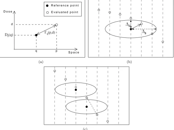
q p d D o s e S p a c e E v a l u a t e d p o i n t R e f e r e n c e p o i n t (a) (b) (c)

Figure 1: Schematic representation of the γ-index. Black (resp. white) points symbolize reference (resp. evaluated) points. The points are drawn in the dose-space domain: the vertical axis stands for dose and the horizontal axis stands for the 1D space. (a) The distance Γq(p, d)in the dose-space domain. (b) The

γ-index of a reference point is the distance in the dose-space domain between this point and the closest point of the evaluated dose. It is less than one if the closest point is inside the ellipsoid around the reference point. (c) Possible presence of false positives: the lower ellipsoid does not contain an evaluated point, though an interpolation between the points of the evaluated dose would pass over it. Thus an error is wrongly reported by the non-interpolated γ-index.

It totally removes the errors in high gradient regions. However the time of computation remains very high since γ-distributions are computed within two minutes on 250 ∗ 250 ∗ 50 grids.

Other methods have been proposed that entirely perform the comparison in the dose domain using both dose-difference and distance-to-agreement criteria [10, 11, 12]. It has been suggested, for example, to adapt the dose-difference method to take the local dose gradient into considera-tion [12]. Another such method is the χ-evaluaconsidera-tion [10], derived from the γ-index, that uses the γ-ellipsoids and the local dose gradient to build an acceptance tube around the reference dose. The main problem of this method is that using only the local gradient makes it inaccurate in the case of non-zero second derivatives [10], thus a more accurate method is needed.

The method proposed in this paper is based on the same idea as the χ-method, in that it computes the minimal and maximal permitted doses at a given position, in order to entirely perform the comparison in the dose domain. These dose-difference tolerances are obtained from the union of all the γ-ellipsoids, and form a region that wraps the reference distribution and that we call the δ-envelope. This method is presented in Section 2.2. Three indexes, called δa, δb and

δc, are then presented in Sections 2.3, 2.4 and 2.5, to show how the envelope concept can be useful

to evaluate the quality of dose distributions. Once the δ-envelope is computed, the comparison of the two distributions by means of the δ-indexes is as fast as a classic dose-difference comparison. This method also avoids the problems of the γ-index in steep dose gradient regions.

The δ-envelope and δ-indexes are then applied to 1D, 2D and 3D test cases, and are evaluated in comparison with the γ-index (Section 3). They turn out to be very accurate and also to be much faster than the classical techniques used to compute the γ-index.

2

MATERIALS AND METHODS

2.1

The

γ-index

This section presents the γ-index [5] and analyses its drawbacks. This method compares two dose distributions, named the reference dose Dr and the evaluated dose De, by combining the

dose-difference and distance-to-agreement criteria. These criteria are denoted by ∆d for the

dose-difference and by ∆s for the distance-to-agreement (“s” stands for “space”).

We denote by Γq(p, d) the distance in the dose-space domain (Fig. 1(a)) between the reference

dose point at position q where the dose is Dr(q), and a point at position p where the dose is d.

This distance is normalized on ∆sand ∆d:

Γq(p, d) = s ||q − p||2 ∆2 s +(Dr(q) − d) 2 ∆2 d , (1)

where ||p − q|| is the Euclidian distance between positions p and q.

The surface representing the acceptance criterion around the point (q, Dr(q)) of the reference

dose is an ellipsoid (Fig. 1(b)) defined by the equation

1 = Γq(p, d). (2)

The γ-index of the point at position q of the reference dose Dris the minimal distance to a

point of the evaluated dose De(see Fig. 1(b)):

γ(q) = min

p {Γq(p, De(p))} . (3)

The point at position q of the reference dose is accepted if γ(q) 6 1, i.e. if the closest evaluated point is inside the ellipsoid, and rejected if γ(q) > 1, i.e. if the closest evaluated point is outside the ellipsoid.

The γ-index, as introduced by Low et al. [5], is widely used in research departments and clinics since it is the first method that proposes a single criterion based on both dose-difference and distance-to-agreement criteria. However some problems exist with this method, as explained in the following paragraphs.

The first problem is well known: in regions of high dose gradient, the γ-index may erroneously be greater than one [8, 9, 10], as an error is reported on a point of the reference dose although it is actually valid. This false error detection is called a false positive. Such a situation is described in Fig. 1(c), where the lower ellipsoid does not contain a point of the evaluated dose whereas the two distributions are very close together. This may happen when ∆d is small and the dose

gradient is steep. Methods have been proposed to filter out these falsely reported unaccepted points [8, 9], but at the expense of computation time. Henceforth these methods will be called interpolated γ-index, while the initial γ-index version proposed in [5] will be referred to as the non-interpolated γ-index.

The second drawback of the γ-method is the necessity to search for the point of the evaluated dose that is the closest to a given reference point. This task can be time consuming in the case of 3D dose distributions. For this purpose fast methods have been developed [6, 7, 8], but a search for each reference point is still needed. A more promising approach is to precompute dose tolerances in order to quickly perform the dose evaluation afterwards. Such an approach is used by the χ-evaluation [10]. It constructs a tube around the reference dose (see Fig. 2(a)) by extending the ellipsoid in the direction of the local dose gradient, also avoiding some false positives. The problem is that this technique is incorrect for non-zero second derivatives, i.e. when the dose gradient varies, because it is only based on the local dose gradient, as it can be seen Fig. 2(b). The method introduced in this paper also precomputes dose tolerances from the reference distribution, but it accurately takes gradient variations into account.

This analysis of the γ-index shows that there is a need for a distribution comparison method that would be reliable (i.e. without false positives) and faster than the γ-index technique. Such method is proposed in this paper. It is based on the δ-envelope concept, that is introduced in the next section.

2.2

The

δ-envelope

A problem of the γ-index shown in the previous section is the presence of false positives: some errors can be falsely reported because there is no evaluated point in the ellipsoid of a reference

(a)

P

(b)

Figure 2: Graphical representation of the χ-evaluation method [10]. (a) The acceptance tube thickness at a position is given by extending the ellipsoid of the reference point at this position in the direction of the local dose gradient. (b) The gradient can vary in the neighborhood of the reference point where the tube is calculated. The evaluated point P is declared incorrect by the χ-evaluation method because it is outside the tube, whereas it is actually valid since it is between two ellipsoids.

point, however there are some evaluated points inside the acceptable dose interval for this po-sition, i.e. evaluated points that stand between the minimal and maximal doses allowed (see Fig. 1(c)). The method proposed here computes these maximal and minimal doses from the γ-ellipsoids of all the reference points, as illustrated in Fig. 3(a), to form what we call the δ-envelope. The maximal (resp. the minimal) dose considered as correct at position p is the maximal (resp. minimal) dose attained by the ellipsoid of a reference point in the neighborhood of p. Thus the tolerances above and below the reference dose at a position p, that are called ε+_{(p) and ε}−_{(p) respectively (see Fig. 3(b)), can be computed by}

ε+(p) = max q,||p−q||≤∆s    Dr(q) − Dr(p) + ∆d s 1 − ||p − q|| 2 ∆2 s    (4) ε−(p) = min q,||p−q||≤∆s    Dr(q) − Dr(p) − ∆d s 1 − ||p − q|| 2 ∆2 s    (5) where ∆d s 1 −||p − q|| 2 ∆2 s

is the dose value on the γ-ellipsoid contour, at a distance ||p − q|| (in the space domain) of its center. It can be directly derived from Eq. (1) where it is the absolute value of Dr(q) − d when

Γq(p, d) = 1.

We introduce e(p) as the dose-difference error at position p:

e(p) = De(p) − Dr(p). (6)

The distribution comparison performed by the γ-index in dose and space domains can now be converted into a comparison in the dose domain only. One can notice that ε−(p) 6 0 and ε+_{(p) > 0 for each position p. As it can be seen in Fig. 3(b), the evaluated point at position p}

is in the envelope if ε−_{(p) 6 e(p) 6 ε}+_{(p), i.e. if D}

e(p) is greater than Dr(p) + ε−(p) and lower

than Dr(p) + ε+(p).

What makes the envelope concept so interesting is that it avoids the need for interpolation that is the main problem of the γ-index. This property comes from the acceptation of all the evaluated points that are inside the envelope, i.e. that are located between the minimal and maximal accepted doses at position p. An evaluated point located inside the envelope has to be accepted because there is necessarily a point of the reference dose (or a point resulting from interpolation between points of the reference dose) of which the γ-ellipsoid contains the evaluated point (see Fig. 3(a) and 3(c)).

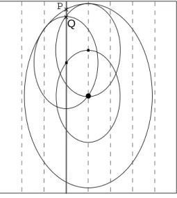
The only problem of the δ-envelope can arise when the resolution is sparse, as can be seen in Fig. 3(d) where an evaluated point is not between the maximal and the minimal ellipsoids, but it would be between them if the reference points were more closed together. This situation can happen in high gradient regions where there is no reference point at a distance about ∆sof the

(a) (b)

(c)

P Q

(d)

Figure 3: (a) The δ-envelope is defined by the minimal and maximal doses attained by the γ-ellipsoids. (b) The δ-envelope at a position p is the dose interval between Dr(p) + ε−(p) and Dr(p) + ε+(p). (c)

The major part of the false positives are directly avoided: the points of the evaluated dose that have an ellipsoid above them and another one below are reported as correct by the δ-envelope method, contrary to the non-interpolated γ-index that reports an error in this example because the lower ellipsoid does not contain a point of the evaluated distribution. (d) The δ-envelope thickness can be underestimated in the case of a sparse distribution, if the dose gradient is steep at a distance ∆s from the point of interest

and if there is no reference point at this position. This is the case in this example where the point P is not in the envelope. An interpolation would then be required to ensure the completeness of the envelope. In this example the point Q would result from the interpolation, so that the point P would be inside the enlarged envelope.

reference point where the envelope is computed (see Fig. 3(d)). In this configuration, the steep gradient at distance ∆s from the reference point is not considered and the envelope thickness

is slightly underestimated. As shown in Fig. 3(d), interpolations could be used to ensure the completeness of the envelope. However this problem can only affect the external border of the envelope. As a consequence, the interpolations are not strictly necessary since they would be of little consequence on the envelope thickness. That is why the evaluations of the δ-envelope presented in Section 3 were performed without interpolation.

In this paper three indexes are presented that take advantage of the δ-envelope concept to provide valuable information about the evaluated distribution De. These indexes are called δa,

δb and δc. Henceforth the expression “δ-indexes” will be used to refer to the three indexes at a

time, and the symbol δ will be used in the equations valid for each δ-index.

2.3

The

δ

-index: a direct application of the envelope concept

The δ-envelope provides the minimal and maximal dose values allowed at each position in the phantom. This information can be used to measure the quality of the evaluated dose distribution De. The direct application of the envelope concept consists in dividing the errors by ε+ or ε−

depending on whether the error is positive or negative:

δa(p) =

( e(p)

ε+_(p) if e(p) > 0

−εe(p)−(p) if e(p) < 0

(7)

If De is inside the envelope at position p, then δa(p) ∈ [−1; 1] (see Fig. 4). If |δa| = 1, then

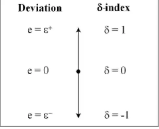
Figure 4: Schematic representation of the δ-indexes. If De(p) is inside the envelope defined around

Dr(p), then δa(p) = δb(p) = δc(p), and −1 6 δ(p) 6 1. If De(p)is outside the envelope, then |δ(p)| > 1

and an error is reported.

As a consequence, |δa| = 1 corresponds to γ = 1, thus either δa or γ can be used to see which

points are rejected and which points are accepted. However, the points rejected by the γ-index are not exactly the same as those rejected by the δa-index (and by δb and δc). The first reason is

that the δ-envelope can be slightly underestimated when it is computed without interpolation, as explained in Section 2.2. But the main reason is that while γ gives the shortest distance between a reference point and the evaluated distribution, the method proposed in this paper calculates the deviation of each point of the evaluated distribution. As a consequence, these two methods can report the same deviation but at nearby locations. Another possible consequence is that some large deviations on the evaluated distribution can be missed by the γ-index, since it does not necessarily use all the points of the evaluated distribution.

The δa-index is well fitted when the evaluated dose is inside the δ-envelope. However, when

the evaluated dose fails both dose and space criteria, i.e. when |δa| > 1, its magnitude can

importantly differ from that of γ. The reason is that the values of ε+(p) and ε−(p) are computed by using the points at distances less than ∆sfrom p, thus the dose gradient variations at distances

greater than ∆sare not taken into account by the δa-index. This is clearly explained in Fig. 5(a),

where one can see that δa shows discrepancies for large deviations (δa> 1) in regions where the

dose gradient changes. However this problem only impacts the large deviations. Then δa can be

a very useful tool, as shown by the evaluation cases in Section 3.

2.4

The

δ

-index: to use

∆

as the maximal spatial uncertainty

The δb-index is the first totally interpretable index based on the δ-envelope. The case where

the evaluated dose is outside the envelope is separated from the case where it is inside. If the evaluated dose is inside the envelope the error is divided by the envelope thickness as in the δa-index. To make the new index coherent outside the envelope, the distance-to-agreement

∆s is now considered as the total spatial uncertainty resulting from all the components of the

treatment chain, i.e. the material, the algorithms and the grid spacing. As a consequence, ∆sis

the maximal spatial deviation that can be tolerated on the evaluated dose, and it cannot be used anymore if the evaluated dose oversteps it. Then in the case where the evaluated dose is outside the envelope, the remaining dose deviation (the deviation minus the thickness of the envelope) is now divided by ∆d. This gives the following definition for the δb-index:

δb(p) =            1 +e(p)−ε_∆d+(p) if ε+_{(p) < e(p)} e(p) ε+_(p) if 0 6 e(p) 6 ε+(p) −εe(p)−(p) if ε −_{(p) 6 e(p) < 0} −1 +e(p)−ε−_(p) ∆d if e(p) < ε −_(p) (8)

As for the δa-index, if Deis inside the envelope at position p, then δb(p) ∈ [−1; 1] (see Fig. 4)

and both dose and space criteria are used in its calculation. If |δb| = 1, then the evaluated dose

is at the limit of the envelope, i.e. at the limit of both dose and space criteria.

If |δb| > 1, the evaluated dose fails both criteria, and the space criterion is not used anymore

(see formula (8)). In that case, δb − 1 gives the dose-difference error remaining outside the

remaining once the spatial uncertainty is exceeded. This information is not provided by the γ-index: when γ > 1, with γ = 1 + β, the value of β comes from both the dose and space criteria, while it may be inappropriate to continue to use the space criterion once it is overstepped.

However, while this index may be very useful to evaluate the importance of deviations in the context of a known spatial uncertainty ∆s, it may be unsuitable when the same information as

γ is needed since the magnitude of δb (like δa) differs from that of γ when De is outside the

envelope. That is why another index is proposed in the next section.

2.5

The

δ

-index: an equivalent to the

γ-index

The δ-envelope boundaries ε+ _{and ε}− _{introduced in Section 2.2 are the limits of both the}

dose-difference and DTA criteria. That is why the γ and δ-indexes are equivalent when the evaluated dose is on the envelope border. In this case γ = δ = 1 (approximately, as explained in Section 2.3). This property will now be extended to make δc equivalent to γ on any integer value. A given

integer value δc = i will correspond to the criteria i∆d and i∆s. With such a definition, δc and

γ can only slightly differ for intermediate values.

To construct this γ-like index, the envelope concept has to be extended. The envelope intro-duced in Section 2.2 only corresponds to the criteria ∆d and ∆s. The envelopes associated with

the criteria i∆d and i∆s for integers i > 0 are now introduced:

ε+i (p) = max q,||p−q||≤i∆s ( Dr(q) − Dr(p) + i∆d s 1 −||p − q|| 2 (i∆s)2 ) (9) ε−i (p) = min q,||p−q||≤i∆s ( Dr(q) − Dr(p) − i∆d s 1 −||p − q|| 2 (i∆s)2 ) (10)

Some remarks can be made about this definition. First of all, for any position p, ε+0(p) =

ε−0(p) = 0. The thickness of the 0-th envelope is null so that it only contains the points of the

reference distribution. Secondly, for any position p, the first envelope (ε+1 and ε−1) is the envelope

introduced in section 2.2.

The direct way to compute these envelopes is to independently compute them. However the time required to compute an envelope linearly depends on the number of points q to evaluate. As a consequence the computation time can become important if ε+i and ε

−

i have to be computed

for large i. A faster method to compute these envelopes is proposed in the annex.

The main advantage of this multi-envelope structure is its equivalence with γ: if the error obtained with the γ-method is such that i 6 γ < i + 1, then the evaluated dose Deis located in

the (i + 1)-th envelope (i.e. ε+_i 6e < ε+_i+1 or ε−_i >e > ε−_i+1). This property is used to construct the δc-index: δc(p) =    i + e(p)−ε + i(p) ε+i+1(p)−ε + i(p) if ∃i ∈ N, ε + i (p) 6 e(p) < ε + i+1(p) −i − e(p)−ε−i(p) ε− i+1(p)−ε − i(p) if ∃i ∈ N, ε − i (p) > e(p) > ε − i+1(p) (11)

To compute the δc-index, we first have to find i > 0 such that the evaluated point is inside

the (i + 1)-th envelope and outside the i-th envelope. Since the number i always remains very small (i 6 2 most of the time), this computation is quasi-instantaneous. In the possible case of large deviations such that several envelopes are necessary, a fast binary search can be used to find i.

The above definition implicitly considers that enough envelopes are precomputed before cal-culating the δc-index, so that every evaluated point is inside an envelope. However, Eq. 11 can

easily be adapted to deal with the case where an evaluated point is outside all the envelopes. For example, if n envelopes were precomputed and if an evaluated point is outside the n-th envelope, δc can be adapted by dividing the remaining dose error by ∆d as with δb. Nevertheless a few

envelopes (two to five) are generally enough because evaluated points that would be outside a too large envelope (for example five times ∆d and ∆s) would be totally unacceptable.

2.6

Analysis

The first advantage of the envelope concept is that it avoids the false positives generated by the non-interpolated γ-index (see Fig. 3(c)). The envelope wraps all the points between the minimal

0 5 10 15 20 25 30 35 0 0.2 0.4 0.6 0.8 1 x (mm) Dose Iso−index δ a D_r (δa = 0) δ_a = ± 1 δ_a = ± 2 (a) 0 5 10 15 20 25 30 35 0 0.2 0.4 0.6 0.8 1 x (mm) Dose Iso−index δ b D r (δb = 0) δb = ± 1 δ_b = ± 2 (b) 0 5 10 15 20 25 30 35 0 0.2 0.4 0.6 0.8 1 x (mm) Dose Iso−index δ_c D_r (δ_c = 0) δc = ± 1 δ_c = ± 2 (c)

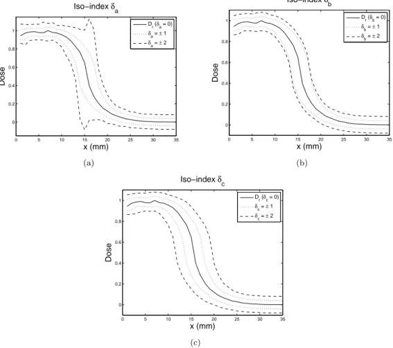
Figure 5: Graphical representation of the iso-indexes curves, with δa, δb and δc taking values in

{−2, −1, 0, 1, 2}. These indexes have the same δ = 0 and δ = ±1 curves, but differ on the δ = ±2 curves. (a) The δa= ±2 curves show discrepancies in regions where the dose gradient varies. (b) The

δb= ±2 curves correspond to the addition of the dose-difference criterion ∆d to the δ = ±1 curves. (c)

The δc= ±2 curves correspond to a 2∆d dose-difference and to a 2∆s distance-to-agreement.

and the maximal tolerated doses so that the points falsely reported as incorrect by the non-interpolated γ-index are caught by the δ-indexes. The only false positives that can remain come from the possible underestimation of the envelope thickness when no interpolation is used (see Section 2.2). However, it is not necessary to use interpolation in the δ-envelopes computation, since this underestimation only slightly modifies the proposed indexes.

Another advantage of the δ-envelopes is that they can be precomputed, so that the calculation of the δ-indexes is approximately as long as a dose-difference test, whereas γ necessitates a search process for each reference point. This makes possible the use of the δ-indexes in situations where the computation time is a key issue, for example in iterative treatment plan optimization. The computational efficiency of the methods proposed in this paper is confirmed by the three-dimensional evaluation presented in Section 3.4.

Another advantage of the δ-indexes is that they give not only the magnitude of the disagree-ment but also its sign, so that the user directly knows if the dose is under or overestimated at a given position. However if a user is only interested in the error magnitude, he can use the absolute value |δ| that reports the same errors as the interpolated γ-index with the advantage that it avoids its other problems, as previously detailed.

It is also worth comparing the δ-indexes to the χ-evaluation method [10]. Contrary to the χ-evaluation that is only based on the local dose gradient (see Fig.2(b)), all the reference points at a distance less than i∆s from p participate in the computation of the i-th envelope. Thus,

contrary to the χ-evaluation method, the method proposed in this paper is appropriate in regions where the dose gradient changes.

Now we focus on the interpretation of the δ-indexes. Since δa = δb= δcif the evaluated point

is inside the first envelope, these indexes accept and reject the same points. Where they differ is in the way they deal with large deviations, i.e. the deviations such that the evaluated point is

outside the envelope.

The δa-index is the most simple application of the δ-envelope concept. Therefore it is very

easy to code and to interpret. Another consequence of its simplicity is that it can be computed as fast as a classic dose-difference test (less than one second on large dose grids, see Section 3.4). However, since it uses the δ-envelope thickness even outside of it, δais not precisely interpretable

for large deviations in regions where the dose gradient changes (see Fig. 5(a)). Then the users interested in precise interpretation of large deviations have to choose either the δb or δc-index.

The δb-index uses the DTA threshold as the maximal tolerated spatial deviation beyond which

only the dose-difference errors are considered. It can be used when ∆sis the only spatial deviation

that can be accepted, and when we are interested in the remaining dose-difference deviation. In such a context, the problem of the γ-index is that it also uses the DTA criterion when γ > 1, thus it implicitly attenuates the deviations. Therefore the δb-index has to be preferred to the

other indexes when ∆s is known to be the maximal tolerated spatial deviation.

The δc-index was designed for situations where greater spatial shifts are admissible. Thus

it provides an equivalent to the γ-index, with the advantage that it avoids its problems of interpolation and of computation time. However δcrequires the computation of several envelopes.

Even though these envelopes can be rapidly computed by the method proposed in the annex, the computational cost is slightly increased (compared with δa and δb that require only one

envelope). Nevertheless, when the reference dose is known in advance, so that the envelopes can be precomputed, δc can be obtained within two seconds on large dose grids, as detailed in

Section 3.4

To summarize, the choice of which index to use mainly depends on the kind of information desired about the large deviations. However, if the calculation time is a key issue and if the reference dose is not known in advance, then δa and δb have to be considered rather than δc.

But when the reference dose is known in advance so that the envelopes can be precomputed, δc is approximately as fast as δa and δb. The computational efficiencies were evaluated on a

three-dimensional test case that is presented in Section 3.4.

3

RESULTS

3.1

Evaluation distributions

The evaluation of the δ-indexes and their comparison to the γ-index were firstly performed on 1D dose distributions to illustrate the envelope concept possibilities, and secondly on 2D distributions to show the advantages of a δ-map. A full 3D computation was also performed to evaluate the computational efficiency of the proposed methods. The dose distributions were computed by the Penelope Monte Carlo code [13]. The voxel size is 1mm.

In the first example (Section 3.2 and Fig. 6), the reference dose Dr is a part of the dose

profile of a 1 × 1cm2_{, monoenergetic 5M eV photon beam entering in a water cubic phantom.}

The distribution used as evaluated dose Deresults from both a 0.5mm shift and a multiplication

by 0.95 of the reference distribution, so that these distributions are slightly different in both dose and space domains. The dose-difference and DTA criteria used are 3% of the maximal dose and 1mm respectively. The γ-index was evaluated with and without interpolation, in order to point out the discrepancies obtained by the direct application of the γ-method, and to show that the δ-method accurately removes these discrepancies.

The beam used in the 2D case (Section 3.3, Fig. 7 and Fig. 8) is the same as in the 1D example. The reference distribution Dris the profile at 2cm depth, normalized to the maximum

dose. The distribution used as evaluated dose De results from both a 2mm shift to the bottom

and a 1mm shift to the right. The dose-difference and DTA criteria used are 3% of the maximal dose and 2mm respectively.

A 3D test case is also presented (Section 3.4) to evaluate the computational cost of the δ-envelopes and δ-indexes. Their efficiency is compared to that of the geometrical γ-computation technique proposed in [8].

3.2

1D Evaluation

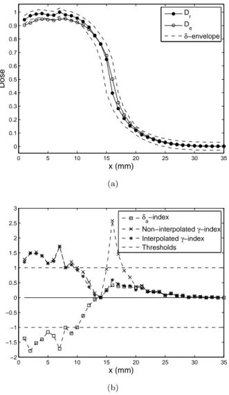
Fig. 6(a) shows the reference (Dr) and evaluated (De) distributions, along with the acceptance

δ-envelope - computed via Eq. (4) and (5) - around Dr. We immediately note that the envelope

thickness can be very high where the dose gradient is steep. For instance, at position x = 16, the accepted dose-difference ε+ _{is equal to 25% of the maximal dose. We can also notice that the}

0 5 10 15 20 25 30 35 0 0.1 0.2 0.3 0.4 0.5 0.6 0.7 0.8 0.9 1 Dose x (mm) D r D e δ−envelope (a) 0 5 10 15 20 25 30 35 −2 −1.5 −1 −0.5 0 0.5 1 1.5 2 2.5 3 x (mm) δ_a−index Non−interpolated γ−index Interpolated γ−index Thresholds (b)

Figure 6: (a) Reference and evaluated distributions, along with the δ-envelope contours. (b) δ and γ-distributions. The dashed line stands for the acceptance limits.

This shows that neither fixed [3, 14] nor symmetric [3, 10, 14] dose-difference tolerances can accurately model the distance-to-agreement criterion in high gradient regions.

Fig. 6(b) shows the γ and δ-indexes for the distributions presented Fig. 6(a). In this example the dose Deis never outside the envelope in steep gradient regions, so that the differences between

the three δ-indexes are very small. That is why δa is the only index represented, for the sake of

clarity. On the other hand, both interpolated and non-interpolated γ-distributions are shown, to highlight the problems of the non-interpolated version and to confirm the accuracy of the δ-envelope method.

We immediately notice that the δ-index can be either negative or positive, indicating the relative positions of Deand Dr. However the γ-index could also give the sign of the deviation if

another information (such as the γ-angle [6]) was used. In the following, only the magnitudes of the γ and δ-indexes are compared.

The explanations are divided into three parts, respectively corresponding to the region at the left (1 6 x 6 13), to the central region with steep gradients (14 6 x 6 20) and to the right region (21 6 x 6 35).

In the first 13 positions, γ and δa have approximately the same magnitude, and they both

report errors corresponding to the dose underestimation. Since the dose gradient is very low in this region, the γ-index is accurate even without interpolation, so that the two γ-curves are superimposed.

In the right region where the dose gradient is also very low, i.e. after the 21st position, the three indexes declare the evaluated dose as accepted.

However the two γ-curves disagree in the central zone, i.e. between the 14th and the 20th positions. Fig. 6(a) shows that the errors reported by the non-interpolated γ-index are false positives, as described in Fig. 1(c): some reference points do not have an evaluated point in their

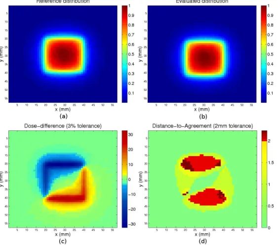
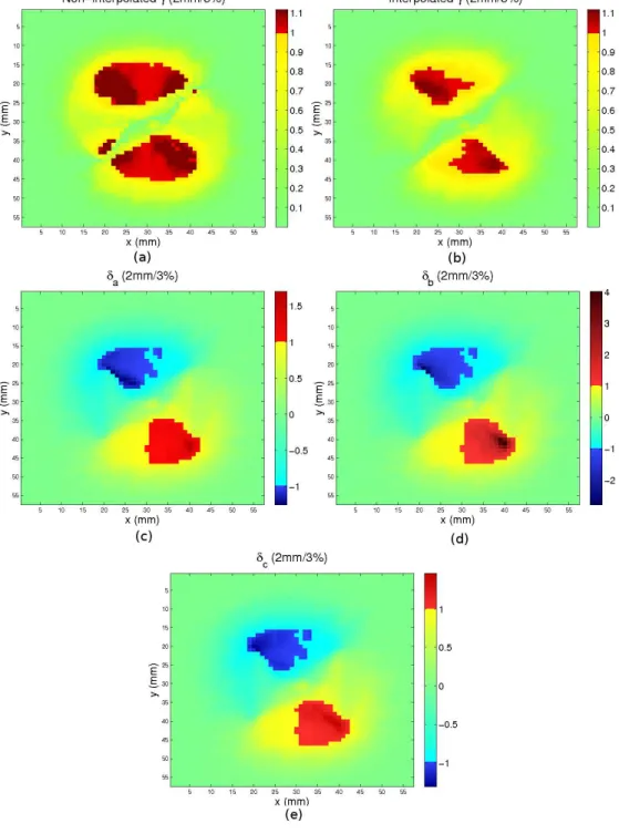
Figure 7: Two-dimensional reference and evaluated distributions, and results of the dose-difference and distance-to-agreement evaluations.

ellipsoid because the evaluated points are located between these ellipsoids, as it can happen in high gradient regions. The envelope method removes these false positives as well as the interpo-lated γ-index. However it has the advantage of being much faster, as explained in Section 3.4.

3.3

2D Evaluation

Fig. 7 and Fig. 8 show the results of some comparison methods for a 2D evaluated distribution (Fig. 7(b)) obtained by shifts to both the right and the bottom from the reference distribution (Fig. 7(a)). The dose-difference and the distance-to-agreement tests, along with the γ (interpo-lated and non-interpo(interpo-lated) and δ-indexes, are the methods compared in this example. Since the evaluated dose is the result of two shifts on the reference dose, it is expected that the DTA test, and more particularly the γ and δ-methods, show smaller errors than the dose-difference test.

As expected, large deviations are shown by the dose-difference test (Fig. 7(c)), up to 32% of the maximum dose. With a 3% tolerated deviation, a great number of points, mainly located in steep gradient regions at the contour of the square field, are rejected by this test. Since the shifts are from left to right and from top to bottom, the dose-difference is negative in the upper-left part and positive in the lower-right part. It can also be noticed that no important error occur at the center and outside the field, because of a low gradient in these regions.

While the dose-difference test finds deviations about 32% (i.e. about 11 × ∆d), the DTA test

does not find more than about 1.1 × ∆s = 2.2mm. The reason is that the evaluated dose was

obtained by shifts from the reference distribution, in such a way that very high dose-difference errors appear in steep gradient regions. One can notice that the 2.2mm value comes from both the 2mm and 1mm shifts (√22_{+ 1}2 _{≈ 2.2). Another difference is that contrary to the}

dose-difference test, the DTA evaluation with 2mm threshold does not show errors on the left and right borders. The reason is that while the shift is 2mm to the bottom, it is only 1mm to the right.

Both the interpolated and non-interpolated γ-indexes are presented (Fig. 8(a) and 8(b)). As expected, more deviations are shown by the non-interpolated version than by the interpolated

Figure 8: Two-dimensional γ and δ-evaluations of the dose distributions shown in Fig. 7.

one. These are false positives (see Section 2.1). Then the following observations are made on the interpolated γ-index. The maximal reported γ-value is about 1.1. This value directly comes from the 2.2mm maximal distance-to-agreement reported in Fig. 7(d) (because 2.2/∆s= 1.1).

The δ-distributions are shown in Fig. 8(c), 8(d) and 8(e). These three indexes accept and reject the same points, because δa = δb = δc when the evaluated distribution is inside the first

envelope. Differences between these indexes only arise when the evaluated distribution is outside the envelope, i.e. for large deviations. It can also be noticed that the points rejected by the γ-index are not exactly the same as those rejected by the δ-indexes, as explained in Section 2.3. The first reason is that the δ-envelope thickness can be slightly underestimated because it is computed without interpolation, and the other reason is that the γ and δ-methods can report the same deviation at close but different locations (see Section 2.3).

The differences between δa and γ are underlined in the lower right region: while the γ-index

shows a 1.1 maximal value, some δa values are greater than 1.6. The reason is that the dose

not precisely processed by the δa-index (see Fig. 5(a)). However this example shows that δa is

sufficient to rapidly evaluate which evaluated points are rejected or accepted.

While the γ-index shows a 1.1 maximal value, the maximal δb-value is 4. The reason is that

while the γ-index gives the lowest dose-space distance between the two curves, the δb-index uses

the space criterion ∆s as the maximal tolerated spatial deviation, so that if the error exceeds

this tolerated spatial deviation (i.e. if the evaluated dose is outside the envelope), the remaining dose deviation is divided by the dose tolerance ∆d (see Eq. (8)). In the current case, a δb

-value of 4 indicates that even with a tolerated 2mm spatial uncertainty, a 3 × ∆d dose error

remains. In this case, if the user knows that the total spatial uncertainty on the whole radiation therapy equipment is 2mm, then he can immediately conclude that the obtained errors are totally unacceptable.

The δc-index was designed to provide an equivalent to the γ-index, in that δc is equal to γ

when the evaluated dose is on the border of one of the envelopes. But their values can slightly differ when the evaluated dose is not on the contour of an envelope, i.e. when γ and δc does not

have integer values. This is clearly illustrated in this example, where the maximal value of δc is

1.4, whereas the maximal value of γ is 1.1. However the differences between these two indexes are large only at a few locations, while they remain very small elsewhere.

This example brings to light the possibilities offered by the use of the δ-envelope concept. The δc-index seems to be the most fitted for people used to the γ-index, since it provides the

same information in spite of small differences in magnitude. The δb-index provides different but

interesting information, in that it evaluates the dose-difference error remaining once the DTA threshold is exceeded. Then it can be used when ∆sis the maximal tolerated spatial uncertainty.

To conclude, even if the δa-index is not perfectly precise in the case of large deviations in regions

where the dose gradient changes (see Fig. 5(a)), this example shows that it can nevertheless be used to evaluate dose distributions, taking advantage of both its simplicity and its computational efficiency.

3.4

3D Evaluation: computation time

A full 3D computation was performed to evaluate the time for computing the envelopes and the δ-indexes. These evaluations were performed with Matlab on a 3.2GHz Intel Xeon, with a 250 × 250 × 50 grid in order to compare the results with those obtained in [8].

The computation of the first envelope took 8.2 seconds. Then the time required to com-pute δa was 0.4s, while the δb computation took 1.2s. Thus the computation of δa and δb is

quasi-instantaneous if the reference dose is known in advance so that the first δ-envelope can be precomputed. In the case of a reference dose not known in advance, the total computa-tion remains very fast (less than 10 seconds) in comparison with the two minutes taken by γ computations in [8].

The computation of the δc-index requires several envelopes, as explained in Section 2.5.

Even though the number of necessary envelopes generally remains small, their computation via Eq. 9 and 10 can be expensive because of the large number of points explored. Thus the fast method described in the annex for constructing the δ-envelopes was used. With this method each envelope is computed as fast as the first envelope. As a consequence, in our test case the time for computing n envelopes was 8.2n seconds. For example, with five envelopes, the computation took about 41 seconds, which remains very reasonable. However five envelopes will be most of the time unnecessary, since either a 5∆d or a 5∆serror would be unacceptable in the context of

radiotherapy.

When the reference dose is known in advance, so that the envelopes can be precomputed, the δc-index is computed in 1.9 seconds on the 250 × 250 × 50 grid.

To summarize, all the indexes proposed in this paper can be computed in less than two seconds on a 3D grid if the reference dose is known in advance. This makes possible to rapidly obtain an index based on both the dose-difference and the distance-to-agreement criteria.

4

CONCLUSIONS

A new tool for the evaluation of dose distributions is presented in this paper. It is based on the same formalism as the γ-index [5], but while γ makes a search for each reference point, the proposed δ-indexes evaluate the distribution by comparison to precomputed dose-difference tolerances. These tolerances are given by the δ-envelope, that comes from the union of the γ-ellipsoids centered on the reference points.

P Q

Figure 9: Approximation made by the fast computation of the list of envelopes. The envelope thickness is computed on the position represented by the bold line, from the reference point at the center of the figure. Small ellipsoids corresponding to ∆dand ∆s are used instead of that corresponding to 2∆d and

2∆s. This can cause small deviations: the envelope thickness is slightly underestimated by the fast

method with small ellipsoids, that provides the point Q whereas the precise computation with the large ellipsoid provides the point P .

Since the δ-envelope wraps the points around the reference distribution, the false positives obtained by the non-interpolated γ-evaluation [5] are directly avoided. Even though methods exist that compute accurate γ-distributions [8, 9], the δ-envelope method directly solves this problem with the benefits of both simplicity and computation time.

If the reference distribution is known in advance, the δ-method can also be speeded up by precomputing the necessary envelopes. In this case, the proposed δ-indexes can be computed in less than two seconds on a 3D grid.

For all these reasons, the δ-method appears to be a very promising tool for the evaluation of dose distributions. Choosing this method will permit to avoid the weaknesses of the γ-index, with no need to change established work habits, since the δ-indexes can be used and displayed exactly in the same way as the γ-index.

Appendix: A fast recursive method for computing the list of

envelopes

The δc-index proposed in Section 2.5 requires the computation of n envelopes (ε+i, ε − i )16i6n

defined in Eq. 9 and 10. These envelopes could be computed independently but the time of calculation becomes important if ε+i and ε

−

i have to be computed for a large i (see explanations

in Section 2.5). In this section a faster method is proposed to compute these envelopes.

The first and second envelopes are represented in Fig. 5(c). While the first one corresponds to a δc = 1 deviation, the second corresponds to a δc = 2 deviation. The technique presented

here computes the second envelope from the first one, and more generally computes the (i + 1)-th envelope from the i-th envelope.

First of all, ε+₀ = ε−₀ = Dr, as stated in Section 2.5, thus the 0-th envelope is directly available.

Then the construction of the first envelope (ε−₁ and ε+₁) from the reference dose distribution Dr

(i.e. from the 0-th envelope) is described in Section 2.2. One can see in Fig. 5(c) that this process can be used to compute the second envelope from the first one, and to compute the (i + 1)-th envelope from the i-th envelope, for each i > 0, in the following way:

ε+_i+1(p) = max q,||p−q||≤∆s    ε+i (q) − ε + i (p) + ∆d s 1 − ||p − q|| 2 ∆s2    (12) ε−i+1(p) = min q,||p−q||≤∆s    ε−i (q) − ε − i (p) − ∆d s 1 − ||p − q|| 2 ∆s2    (13)

With this method, all the points at a distance less than ∆s from p are explored during the

computation of the (i+1)-th envelope at position p. This is exactly the same area as in the δ-envelope computation proposed in Section 2.2. Thus the computation of the n δ-envelopes (from ε+1

to ε+

n and from ε−1 to ε−n) is as long as n computations of the δ-envelope proposed in Section 2.2.

However, in the case of a sparse grid spacing, this method does not provide the exact en-velopes. Small discrepancies may appear because the large ellipsoids used in Eq. 9 and 10 cannot perfectly be substituted by the small ellipsoids used in the method presented in this section (see Fig. 9). Then some errors can appear on ε+i and ε

−

i for i > 2. However these errors only slightly

affect the external borders of the envelopes, thus the indexes calculated from these envelopes are not importantly modified. It can also be noticed that these errors are additive, so that the error on the (i + 1)-th envelope will always be larger than the error on the i-th envelope. However, a very high precision is not necessary when the deviation becomes important. For example, no one would perceive the difference between δc = 3.9 and δc = 4.1. In this case the user only has

to be aware of a deviation about four times larger than the threshold.

Acknowledgement

The authors would like to thank the reviewer for a thorough examination of our paper and helpful suggestions.

References

[1] A. Van Esch, J. Bohsung, P. Sorvari, M. Tenhunen, M. Paiusco, M. Iori, P. Engström, H. Nyström, and D.P. Huyskens. Acceptance tests and quality control (qc) procedures for the clinical implementation of intensity modulated radiotherapy (imrt) using inverse planning and the sliding window technique: experience from five radiotherapy departments. Radiother. Oncol., 65:53–70, 2002.

[2] B.E. Nelms and J.A. Simon. A survey on planar imrt qa analysis. J. Appl. Clin. Med. Phys., 8:76–90, 2007.

[3] J. Van Dyk, R.B. Barnett, J.E. Cygler, and P.C. Shragge. Commissioning and quality assurance of treatment planning computers. Int. J. Radiat. Oncol. Biol. Phys., 26:261–73, 1993.

[4] W.B. Harms, D.A. Low, J.W. Wong, and J.A. Purdy. A software tool for the quantitative evaluation of 3d dose calculation algorithms. Med. Phys., 25:1830–36, 1998.

[5] D.A. Low, W.B. Harms, S. Mutic, and J.A. Purdy. A technique for the quantitative evalu-ation of dose distributions. Med. Phys., 25:656–61, 1998.

[6] M. Stock, B. Kroupa, and D. Georg. Interpretation and evaluation of the gamma index and the gamma index angle for the verification of imrt hybrid plans. Phys. Med. Biol., 50:399–411, 2005.

[7] M. Wendling, L.J. Zijp, L.N. McDermott, E.J. Smit, J.-J. Sonke, B.J. Mijnheer, and M. Van Herk. A fast algorithm for gamma evaluation in 3d. Med. Phys., 34:1647–54, 2007.

[8] T. Ju, T. Simpson, J. O. Deasy, and D. A. Low. Geometric interpretation of the gamma dose distribution comparison technique: Interpolation-free calculation. Med. Phys., 35:879–87, 2008.

[9] T. Depuydt, A. Van Esch, and D.P. Huyskens. A quantitative evaluation of imrt dose distributions refinement and clinical assessment of the gamma evaluation. Radiother. Oncol., 62:309–19, 2002.

[10] A. Bakai, M. Alber, and F. Nüsslin. A revision of the gamma-evaluation concept for the comparison of dose distributions. Phys. Med. Biol., 48:3543–53, 2003.

[11] S.B. Jiang, G.C. Sharp, T. Neicu, R.I. Berbeco, S. Flampouri, and T. Bortfeld. On dose distribution comparison. Phys. Med. Biol., 51:759–76, 2006.

[12] J.M. Moran, J. Radawski, and B.A. Fraass. A dose-gradient analysis tool for imrt qa. J. Appl. Clin. Med. Phys., 6:62–73, 2005.

[13] F. Salvat, J.M. Fernandez-Varea, E. Acosta, and J. Sempau. Penelope-2006, a code system for monte carlo simulation of electron and photon transport. In NEA 6222, ISBN: 92-64-02301-1, 2006.

[14] J. Venselaar, H. Welleweerd, and B. Mijnheer. Tolerances for the accuracy of photon beam dose calculations of treatment planning systems. Radiother. Oncol., 60:191–201, 2001.