Tourism, jobs, capital accumulation and the economy: A dynamic analysis

HAL Id: halshs-00590811

https://halshs.archives-ouvertes.fr/halshs-00590811

Preprint submitted on 5 May 2011

HAL is a multi-disciplinary open access

archive for the deposit and dissemination of sci-entific research documents, whether they are pub-lished or not. The documents may come from teaching and research institutions in France or

L’archive ouverte pluridisciplinaire HAL, est destinée au dépôt et à la diffusion de documents scientifiques de niveau recherche, publiés ou non, émanant des établissements d’enseignement et de recherche français ou étrangers, des laboratoires

Tourism, jobs, capital accumulation and the economy: A

dynamic analysis

Chi-Chur Chao, Bharat R. Hazari, Jean-Pierre Laffargue, Pasquale M. Sgro,

Eden S. H. Yu

To cite this version:

Chi-Chur Chao, Bharat R. Hazari, Jean-Pierre Laffargue, Pasquale M. Sgro, Eden S. H. Yu. Tourism, jobs, capital accumulation and the economy: A dynamic analysis. 2005. �halshs-00590811�

P

ARIS

-J

OURDAN

S

CIENCES

E

CONOMIQUES

48, BD JOURDAN – E.N.S. – 75014 PARIS TEL. : 33(0) 1 43 13 63 00 – FAX : 33 (0) 1 43 13 63 10

www.pse.ens.fr

WORKING PAPER N° 2005 - 16

Tourism, Jobs, Capital Accumulation and the Economy:

A Dynamic Analysis

Chi-Chur Chao

Bharat R. Hazari

Jean-Pierre Laffargue

Pasquale M. Sgro

Eden S. H. Yu

Codes JEL : O10, F11

Mots clés :Tourism, employment, capital accumulation,

welfare

Tourism, Jobs, Capital Accumulation and the Economy:

A Dynamic Analysis

Chi-Chur Chao a,b, Bharat R. Hazari b, Jean-Pierre Laffargue c, Pasquale M. Sgro b, and Eden S. H. Yu d

a

Department of Economics, Chinese University of Hong Kong, Shatin, Hong Kong b

Deakin Business School, Deakin University, Malvern, Victoria 3144, Australia c

PSE-CNRS and CEPREMAP, Paris, France d

Department of Economics and Finance, City University of Hong Kong, Kowloon, Hong Kong

Abstract: This paper examines the effects of tourism on labor employment, capital accumulation and resident welfare for a small open economy with unemployment. A tourism boom improves the terms of trade, increases labor employment, but lowers capital accumulation. The reduction in the capital stock depends on the degree of factor intensity. When the traded sector is weakly capital intensive, the fall in capital would not be so severe and the expansion of tourism improves welfare. However, when the traded sector is strongly capital intensive, the fall in capital can be a dominant factor to lower welfare. This immiserizing result of tourism on resident welfare is confirmed by the German data.

Résumé: Ce papier examine l’effet du tourisme sur l’emploi, l’accumulation du capital et le bien-être dans une petite économie ouverte où une partie de la main-d’oeuvre est au chômage. Une augmentation des recettes touristiques améliore le terme de l’échange, augmente l’emploi, mais réduit l’investissement. La baisse du stock de capital dépend des intensités en facteurs des productions. Quand le secteur exposé a une intensité capitalistique faible, la baisse du capital reste limitée et l’augmentation des recettes touristique améliore le bien-être national. Cependant, si le secteur exposé a une intensité capitalistique forte, la baisse du capital est plus ample et nous obtenons une diminution du bien-être national. L’effet appauvrissant que peut avoir le tourisme est illustré par des simulations sur données allemandes.

Key words: Tourism, employment, capital accumulation, welfare JEL classifications: O10, F11

1. Introduction

Tourism is a growing and important industry in both developed and developing countries. It is also an important source of earning foreign exchange and providing employment opportunities for domestic labor. Expenditure by tourists in the receiving country is predominantly in non-traded goods and services. This type of consumption had become quite important especially for economies suffering a downturn in their traded-goods sector. The recent recovery of the Hong Kong economy is a good example of this type of tourism led recovery and growth. In the past two decades, due to the restructuring and relocation of manufacturing processes to China, unskilled workers in Hong Kong have borne the brunt of unemployment. The Asian financial crisis in 1997 and the SARS outbreak in 2003 had made the situation even worse and the unemployment rate in Hong Kong reached more than 7 per cent. Since April 2003, China has allowed individuals from selected cities to visit Hong Kong. The consequent tourism boom of 4.26 million visits in 2004 has provided job opportunities and thus substantially reduced unemployment. The economic doldrums was halted and the GDP growth is 8.2 per cent in 2004, well above average 4.8 per cent over the past 20 years.1

A considerable amount of research has concentrated on understanding the effects of tourism on the economy. In the distortion-free static models of Copeland (1991), Hazari and Ng (1993) and Hazari and Sgro (2004), a tourism boom yields a demand push, which immediately raises the price of the non-traded good. Since tourism is considered as exports of services, this gain in the “tertiary terms of trade” improves residents’ welfare. Subsequent research has extended the analysis of the effects of tourism in two directions. The first direction is to examine the static economies with distortions. For example, Hazari, et al. (2003) and Nowak et al. (2003) are in this line of research, where the former analyzes the welfare effect of tourism in a Harris-Todaro (1970), urban unemployment economy, while the later introduces increasing returns to scale in the economy. The second direction of research is on the dynamic impacts of tourism. Using a one-sector economy framework, Hazari and Sgro (1995) found that tourism may be

welfare improving although it can lower capital accumulation. Recently, Chao, et al. (2005) have demonstrated that an expansion of tourism may reduce the capital stock, thereby lowering welfare in a two-sector model with a capital-generating externality.

However, the relationship between tourism and employment remains unexplored, although the employment effect of trade policy in general has been a central issue in the literature [cf. Hatzipanayotou and Michael (1995) and Michael and Hatzipanayotou (1999)]. Does the booming tourism business help create more jobs to the local economy, reduce the unemployment rate and hence improve workers’ welfare? To answer this question, we adopt the minimum-wage model of Brecher (1974) in which economy-wide unemployment exists in the economy. The model is extended to incorporate capital adjustments in the long run. Because of the nature of labor intensity in the tourism industry, the expansion of tourism increases demand for manpower, which increases employment Nonetheless, the expansion of the tourism industry may hurt the other sectors in the economy and may lead to a reduction in capital accumulation. When the traded sector is relatively strong capital intensive to the non-traded tourism sector, the fall in the capital stock plays a dominant factor that can lower economic welfare. Hence, in evaluating the effectiveness of tourism to the economy, a trade off between the gain in labor employment and the loss in capital needs to be considered.

The structure of this paper is as follows. Section 2 sets out a dynamic model with capital accumulation for examining the effects of tourism on the non-traded price, labor employment, capital accumulation and welfare in the short and long runs. Section 3 provides numerical simulations for a boost in tourism on the economy. Section 4 outlines the main findings and conclusions.

2. The Model

We consider a small open economy that produces two goods, a traded good X and a non-traded good Y, with production functions: X = X(LX, KX, VX) and Y = Y(LY, KY, VY). The variables

Li, Ki and Vi denote the amounts of labor, capital and specific factor employed in sector i, i = X, Y.

While both labor and capital are perfectly mobile between sectors, there are specific factors Vi to

each sector.2 So, the model considered is a mixture of the Heckscher-Ohlin and the specific-factors model. Choosing the traded good X as the numeraire, the relative price of the non-traded good Y is denoted by p. The production structure of the model is expressed by the revenue function: R(1, p, K, L) = max {X(LX, KX, VX ) + pY(LY, KY, VY): LX + LY = L, KX + KY = K}, where

L is the amount of labor employment and K is the stock of capital in the economy. The fixed endowments of specific factors Vi are suppressed in the revenue function. Denoting subscripts as

partial derivatives and employing the envelope property, we have: Rp = Y, being the output of

good Y, with a normal price-output relation Rpp > 0. Under the stability condition of the

economy,3 sector Y is required to be labor intensive relative to sector X. This gives: RpL > 0 and

RpK < 0, by the Rybczynski theorem. In addition, letting r be the rental rate to capital, we have RK

= r. Because of the existence of specific factors Vi, we have RKK < 0 and RKL > 0.

4

Furthermore, letting w be the wage rate, the level of total employment is determined by:

RL(1, p, K, L) = w, (1)

where RLL < 0 due to diminishing returns of labor.

5

Note that the wage rate is set by the government based on the prices of the traded and non-traded goods, i.e., w = w(1, p), with ∂w/∂p > 0 and (p/w)(∂w/∂p) ≤ 1. This real wage rigidity caused by the wage indexation results in economy-wide unemployment,

L

- L, where

L

is the labor endowment in the economy.

Turning now to the demand side of the economy, domestic residents consume both goods, CX and CY, while foreign tourists demand only the non-traded good Y. Let DY(p, T) be the

tourists’ demand for good Y, where T is a shift parameter capturing the tourist activity with

∂DY/∂T > 0. The market-clearing condition for the non-traded good requires the equality of its

demand and supply:

This equation determines the relative price, p, of good Y.

In a dynamic setting, domestic savings out of consumption of goods X and Y will be used for capital accumulation:

K

& = R(1, p, K, L) – CX – pCY, (3)

where a dot over a variable is its time derivative. Note that capital is imported with a given world price which is normalized to unity.

Under the budget constraint (3), the domestic residents maximize the present value of their instantaneous utility, U( ⋅ ). The overall welfare W is therefore:

W =

∫

∞ − 0

U

(

C

,

C

)

e

dt

t Y X ρ _{, (4)}

where ρ represents the rate of time preference. Letting λ be the shadow price of capital in the economy, the first-order conditions with respect to CX and CY are obtained as

UX(CX, CY) = λ, (5)

UY(CX, CY) = λp. (6)

In addition, the evolution of the shadow price of capital is governed by

λ

&_{= λ[ρ - R}

K(1, p, K, L)]. (7)

Using the above framework, we can examine the resource allocation and welfare effects of tourism on the economy in the short and long runs.

a. Short-run equilibrium

In a short-run equilibrium,

K

& = 0 in (3) and

λ

&= 0 in (7); the amount of capital K is given by K0 as its shadow price is fixed.

6

For a given value of the tourism parameter T, the system can be solved for L, p, CX and CY by (1), (2), (5) and (6) as functions of K, λ and T. That

is, L = L(K, λ, T), p = p(K, λ, T), CX = CX(K, λ, T) and CY = CY(K, λ, T). An increase in capital,

increase in capital lowers the supply of good Y by the Rybcyznski effect, which raises its price

(∂p/∂K > 0). This lowers the demand for good Y by domestic residents (∂CY/∂K < 0).

Furthermore, for UXY > 0, the decreased consumption of good Y lowers marginal utility of good X,

which reduces the demand for good X (∂CX/∂K < 0). Analogously, a rise in the shadow price of

capital lowers the demand for labor in production (∂L/∂λ < 0) and the demand for goods in consumption (∂CX/∂λ < 0 and ∂CY/∂λ< 0). This causes the fall in the non-tradable price (∂p/∂λ <

0). In addition, a rise in tourism increases the demand for the non-traded good and hence its price

(∂p/∂T > 0). This gives to an increase in employment in the economy, ∂L/∂T > 0. However, the

higher price also reduces the demand for both goods by domestic residents (∂CX/∂T < 0 and

∂CY/∂T < 0).

7

b. Dynamics

We can use the short-run comparative-static results to characterize the local dynamics of the model. The dynamics of domestic capital accumulation in (3) and its shadow prices in (7) are:

K

& = R[1, p(K, λ, T), K, L(K, λ, T)] – CX (K, λ, T) – p(K, λ, T)CY(K, λ, T), (8)

λ

&= λ{ρ – RK [1, p(K, λ, T) , K, L(K, λ, T)]}. (9)

Taking a linear approximation of the above system around the equilibrium, we have:

















λ

& &

K

=

_





M

A







N

B

















−

−

λ

λ

~

~

K

K

(10)

where a tilde (~) over a variable denotes its steady-state level. Note that A = RK + RL(∂L/∂K) +

DY(∂p/∂K) - ∂C/∂K, B = RL(∂L/∂λ) + DY(∂p/∂λ) - ∂C/∂λ,

8

M = -λ[RKK + RKL(∂L/∂K) + RKp(∂p/∂K)]

and N = - λ[RKp(∂p/∂λ) + RKL(∂L/∂λ)]. The signs of A, B, M and N are in general indeterminate.

relatively strong labor intensive, and RLL/RLK < RpL/RpK < RKL/RKK. Furthermore, B > 0 when η =

-(∂DY/∂p)(p/DY) ≥ 1, i.e., the price elasticity of the demand for good Y by tourists is elastic.

λ

λ

&

′

_{= 0} SS

λ

&= 0 S′S′ E E’

K

&= 0 F

K

&

′

= 0 0

K

~

′

K

~

K

Figure 1. An expansion of tourism

The schedules of

K

&= 0 and

λ

&= 0 are depicted in Figure 1 with the slopes of dλ/dK|K =

-A/B < 0 and dλ/dK|λ = - M/N > 0 Under this case, the determinant of the above coefficient

matrix is negative and the steady-state equilibrium is at point E which is a saddle point with one negative and one positive eigenvalue. For the given initial value of the capital stock K0, we can obtain from (10) the following solutions for the capital stock and its shadow price around their steady-state values:

Kt =

K

~

+ (K0 -

K

~

)eµ t, (11) λt =

λ

~

+ θ(Kt -

K

~

), (12)

where θ = (µ - A)/B < 0, and µ is the negative eigenvalue in (10). The stable arm of the relation between K and λ, as shown in (12) and also depicted by the SS schedule in Figure 1, indicates that a decrease in K leads to an increase in its shadow price λ, and vice versa.

c. Steady State

The long-run equilibrium is expressed by the short-rum equilibrium in (1), (2), (4) and (5), together with no adjustments in the capital stock and its shadow price in (3) and (7) as:

R(1,

~

p

,

K

~

,

L

~

) -

C

~

_X–

p

~

C

~

_Y = 0, (13)

RK(1,

p

~

,

K

~

,

L

~

) = ρ. (14)

Equations (1), (2), (4), (5), (13) and (14) contain six endogenous variables,

L

~

,

p

~

,

C

~

_X,

C

~

_Y,

K

~

and

λ

~

, along with a tourism parameter, T. This system can be used to solve for the long-run impacts of tourism on the economy. An increase in the tourism business on the long-run price of the non-traded good Y is:

d

p

~

/dT = S(∂DY/∂T)( p 2 UXX + UYY - 2pUXY)/∆ > 0, (15) where UXX < 0, UYY < 0, and ∆ < 0. 9 Note that S = RKKRLL - 2 KL

R

> 0 by the concavity of the production functions. Hence, an increase in tourism will improve the terms of trade.

In addition, from (1) and (14), we can obtain the long-run effects of tourism on the capital stock and labor employment, as follows:

d

L

~

/dT = = [RpKRKK(RKL/RKK - RpL/RpK)/S](d

p

~

/dT) > 0, (16)

where recalling that RLL/RLK < RpL/RpK < RKL/RKK for stability. An increase in tourism can bring

more labor employment in the long run, but at the expense of capital accumulation in the economy. The reduction in the capital stock can be seen in Figure 1. A boom in tourism shifts both schedules of

K

& = 0 and

λ

&= 0 to the left.10 Since the capital stock is given at time 0, the adjustment path takes from point E to point F. This immediately leads to a fall in the shadow price of capital,11 and consequent reductions in capital accumulation from point F to a new equilibrium at point E′.12

d. Welfare

We are now ready to examine the effect of tourism on overall welfare of the economy. Total welfare in (4) can be obtainable from the sum of the instantaneous utility Z = U(CX, CY).

Following Turnovsky (1999, p. 138), the adjustment path of Z is: Zt =

Z

~

+ [Z(0) -

Z

~

]eµ t, where

Z(0) denotes the utility at time 0. Total welfare is hence: W =

Z

~

/ρ + [Z(0) -

Z

~

]/(ρ - µ), and the

welfare change is: dW = [dZ(0) - (µ/ρ)d

Z

~

]/(ρ - µ), where -µ/ρ (> 0) denotes the discount factor. Utilizing (13), the change of total welfare caused by a tourism boom is:

dW/dT = [λ/(ρ - µ)]{DY[dp(0)/dT - (µ/ρ)(d

p

~

/dT)] + RL[dL(0)/dT - (µ/ρ)(d

L

~

/dT)] – (µ/ρ)RK(d

K

~

/dT)}. (18)

where p(0) and L(0) are the non-traded price and labor employment at time 0. Since the capital stock is given at time 0, a tourist boom immediately increases the demand for good Y and hence its prices. As a consequence, higher labor demand is needed for producing more good Y. These results can be derived from (1), (2), (5), (6) and (13) as

dp(0)/dT = - (∂DY/∂T)RLL(2pUXY - p

2

UXX – UYY)/H > 0, (19)

dL(0)/dT = - (RpL/RLL)(dp(0)/dT) > 0, (20)

The welfare effects of tourism in (18) depend on the changes in the terms of trade, labor employment and capital accumulation. An expansion of tourism increases the initial and steady-state prices of the non-traded good, which yields a gain in the terms of trade as shown in the first term in the curly bracket in (18). While the terms-of-trade effect is known in the literature, the impacts of tourism on labor employment and capital accumulation are of importance to economic welfare. As indicated in second term of (18), tourism can generate more labor employment in the short and the long run via the higher price of the non-traded good. However, the higher price of the non-traded good can reduce the demand for capital, causing a welfare loss as shown in the third term of (18). Due to these conflicting forces, the welfare effect of tourism in (18) is in general ambiguous. In the next section, we will use a simulation method to ascertain the welfare effects of tourism in the short and the long run.

3. Simulations

To calibrate the effects of an increase in tourism on the endogenous variables of the economy, we need to specific functional forms for the utility and production functions.

a. Specifications

We assume Cobb-Douglas functions for the production of the traded and non-traded goods: X = A α1 α2 1−α1−α2 X X X

K

V

L

, (21) Y = B β1 β2 1−β1−β2 Y Y Y

K

V

L

, (22)

where A and B are the constant technology factors, and αi and βi are respectively the ith factor

shares in productions of goods X and Y. Total employment for sectors X and Y in the economy is given by

L = LX + LY, (23)

and total capital in the economy is represented by

K-1 = KX + KY. (24)

Note that capital is inherited from the past and is given in the short run, but it can be freely allocated between both sectors. This is the reason why total capital is indexed by -1 (it is predetermined in the short-run equilibrium) and capital allocation in each sector is not indexed.

Facing the wage rate w, the rental rate r and the non-traded price p, the production sector solves the program: Max X + pY – w(LX + LY) - r(KX + KY), subject to X = A 1 2

α α X X

K

L

and Y = B β1 β2 Y Y

K

L

. Here, the specific factors VX and VY are normalized to unity. The first-order conditions

with respect to Li and Ki yield equilibrium allocation of labor and capital between sectors:

w =

α

₁

₍

_/

₎

α2 α1+α2−1

=

β

₁

(

_/

)

β2 β1+β2−1 Y Y Y X X X

L

L

p

B

K

L

L

K

A

, (25) r =

α

₂

₍

_/

₎

α1 α1+α2−1

=

β

₂

(

_/

)

β1 β1+β2−1 Y Y Y X X X

K

K

p

B

L

K

K

L

A

. (26)

The consequent factor-price frontiers can be deduced from (25) and (26):

A

L

r

w

− 2 2 1_X− 1− 2

=

2 1 1

)

(

/

)

/

(

α

α

α

α α α , (27)

pB

L

r

w

− 2 2 1_Y− 1− 2

=

2 1 1

)

(

/

)

/

(

β

β

β

β β β . (28)

In addition, real wage, denoted by wc, in the economy is assumed to be rigid in the sense

that the wage rate w is indexed to the price of the consumption goods pc:

wc = w/pc, (29)

where pc is defined in (32).

Turn to the demand side of the economy, in which a CES functional form for the instantaneous utility function of domestic households is assumed:

where b ∈ [0, 1] and

b

= 1 – b are the parameters, γ expresses the index of relative risk aversion

and σ captures the elasticity of substitution between the two goods with 1 + σ ≥ 0. From the

first-order conditions of utility maximization, we can derive

bCY/

b

CX = 1/p

(1+σ)

. (31)

Denoting C = [b1/(1+σ)

C

σ_X/(1+σ)+

b

σ/(1+σ)

C

_Yσ/(1+σ)](1+1/σ) as the consumption aggregate of the traded

and non-traded goods, we have C = (CX/b)(b +

b

p-σ)

(1+σ)/σ

. The price of the consumption aggragate is then defined by pcC = CX + pCY, which gives

pc = (b +

b

p-σ)-1/σ. (32)

Therefore, the current utility of domestic households can be expressed as: U(C) = C(1-γ)/(1 - γ) = [(CX/b)(b +

b

p

-σ

)(1+σ)/σ](1-γ)/(1 - γ).

To close the model, we need to consider the market-clearing condition for the non-traded good Y:

CY + DY = Y, (33)

where the demand for the non-traded good by tourists is specified as

DY = T/p

η

, (34)

where η measures the price elasticity of demand for good Y by tourists. Tourists spending T, measured in the traded good, is exogenous and tourists consume only non- traded good.

Finally, the budget constraint for each period is:

K – K-1 + CX + pCY = X + PY. (35)

Note that the balance of payments is in equilibrium for each period. From (33) and (35), we can deduce: K – K-1 + CX – X = pDY. That is, the excess demand for capital and the traded good is

financed by income receipts from tourism.

Total welfare of domestic residents is the discounted sum of the instantaneous utility and it can be written as: W =

Σ

∞_t=0(1 - ρ)t[CX(b +

b

p

-σ

relatively to capital and the consumption of the traded good under the series of budget constraints: K – K-1 + CX(b +

b

p-σ)/b = X + pY = w(LX + LY) + rK-1 + vXVX + vYVY. Solving this

maximisation program with respect to CX and K, we obtain the firstorder conditions: (1

-ρ)t −γ

X

C

(b +

b

p-σ)(1+1/σ)(1-γ)-1 = δ/b and δ - δ+1(1 + r+1) = 0 where δ is the Langrange multiplier. After the elimination of δ and δ+1, we have

(1 + r+1)(1 - ρ) = (CX/CX,+1)

-γ

[(b +

b

p-σ)/(b +

b

p

₊₁−σ )(1+1/σ)(1-γ)-1. (36)

b. Calibrations

Equations (21) – (36) consist of sixteen endogenous variables and a shift parameter of tourist spending T for the economy. We will use the German data to calibrate the short- and long-run impacts of an increase in tourism on the economy. It is assumed that tourists’ spending is 0 in the reference steady state. We choose p = 0.9488, X + pY = 1.3909 and L = 27.27, which represent the averages values of these variables for Germany on the period 1996-2002. Units are in trillion of 1995 euros and in millions of persons. We set: T = 0, σ = - 0.5, b = 1/3, ρ = 0.05, α1 = 0.30, α2 = 0.50, β1 = 0.5, β2 = 0.10, λ = 0.5 and η = 1.

13

Note that the labor intensity of good Y is captured by the chosen values of αi and βi. The steady-state values of the sixteen endogenous

variables can be then computed according to: DY = 0, X = (X + pY)/[1 + (

b

/b)p -σ

], Y = (X + pY –

X)/p, CY = Y, CX = X, r = 1/(1 - ρ) - 1, LY = [β1pY/(α1X + β1pY)]L, L = LX + LY, KY =β2pY/r, B =

Y/ β1 β2 Y Y

K

L

, w = pβ1

B

1/(1−β2)

(

p

β

₂

/

r

)

β2/(1−β2)

L

−_Y(1−β1−β2)/(1−β2), KX = α2X/r, A = X/( 1 2 α α X X

K

L

), U =

[

_{1/(1+σ) σ/(1+σ) 1/(1+σ) σ/(1+σ)}

]

(1+1/σ)(1−γ)

+

Y X

b

C

C

b

/(1 - γ), K = KX + KY, and pc = (b +

b

p -σ )-1/σ. The reference steady state values are therefore: CX = 0.4718, CY = 0.9687, DY = 0, K = 6.2285, KX =

4.4821, KY = 1.7464, L = 27.27, LX = 6.4212, LY = 20.8488, p = 0.9488, pc = 0.9657, r = 0.0526,

There are one anticipated variable CX,+1 and one predetermined variables K-1 in the

system. The eigenvalues in the neighbourhood of the reference steady state are equal to 0.9717 and 1.092. So the local condition of existence and uniqueness are satisfied (one of the eigenvalues must be less than one and the other larger than one to get the existence and uniqueness of a solution). As we will compare the consequences of tourism in the short and in the long run, we simulated the model over 250 periods.14

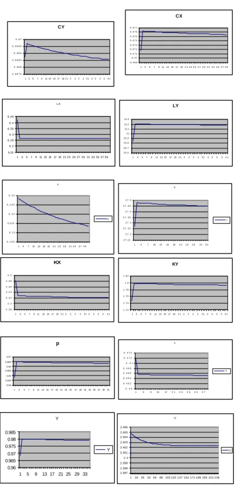
As for reference simulations, we let tourist spending T to increase from 0 to 0.01 (which means by 10 billions euros, the German added value in non-tradable goods being 982 billions euros). We obtain the short- and long-run impacts of tourism on the economy, as plotted in Figure 2:

1. CX and CY immediately increase above their reference values, and then progressively

decrease but CY ends with a level lower than its reference value.

2. LX immediately falls and then slightly increases, while LY immediately rises and then

slightly decreases. This gives that total employment L to rise initially and progressively decreases but stays above its reference level.

3. KX immediately declines and continuously falls, while KY immediately rises and then

declines. However, total K progressively decreases to a lower level.

4. X immediately decreases and then progressively decreases to a lower level, while Y immediately rises and then progressively decreases to a level which is higher than its reference value.

5. p immediately increases above its reference value, and then progressively decreases but stays above its reference value.

6. U immediately increases above its reference value, and then progressively decreases to a

value that is above its reference value. The sum of discounted utilities increases from 343.6305 to 344.0061. Hence, a rise in tourism improves total welfare in the long run.

Consider next the case that the non-traded sector Y is strongly labor-intensive (or weakly capital-intensive) relative to the traded sector X. For this case, we choose β2 = 0.001 and leave the other parameters the same as before. The consequent eigenvalues are 0.9683 and 1.093, and the reference steady-state values are: CX = 0.4718, CY = 0.9687, DY = 0, K = 4.4996, KX = 4.4821,

KY = 0.0175, L = 27.27, LX = 6.4212, LY = 20.8488, p = 0.9488, pc = 0.9657, r = 0.0526, U =

2.4003, w = 0.0220, X = 0.4718 and Y = 0.9687.

Consider reference simulations by increasing tourist spending T from 0 to 0.01. We obtain the short- and long-run impacts of tourism, as plotted in Figure 3. Compared to the results in Figures 2 and 3, the patterns of changes in all the endogenous variables are the same. However, in Figure 3, the rise in total employment L is smaller but the fall in capital K is larger. These differences render a different effect of tourism on utility and welfare: although U immediately increases above its reference value, it progressively decreases and reaches a value below its reference value. Therefore, the sum of discounted utilities decreases from 343.6305 to 343.5839. Thus, owing to the fall in the capital stock, a rise in tourism can lower total welfare when the traded sector is strongly capital-intensive relative to the non-traded tourism sector.

4. Conclusions

Using a dynamic general-equilibrium framework, this paper has examined the short- and long-run effects of tourism on labor employment, capital accumulation and resident welfare for a small open economy with unemployment. A tourism boom improves the terms of trade, increases labor employment, but lowers capital accumulation if the non-traded tourism sector is labor intensive relative to the other traded sector. Nonetheless, the reduction in the capital stock depends on the degree of factor intensity. When the traded sector is weakly capital intensive, the fall in capital would not be so severe and the expansion of tourism improves welfare. However, when the traded sector is strongly capital intensive, the fall in capital can be a dominant factor to

lower total welfare. This immiserizing result of tourism on resident welfare is confirmed by the German data.

CX 0 . 4 6 9 0 . 4 7 0 . 4 7 1 0 . 4 7 2 0 . 4 7 3 0 . 4 7 4 0 . 4 7 5 0 . 4 7 6 0 . 4 7 7 13 5 7 911131517192 1 2 3 2 5 2 7 2 9 3 1 3 3 3 5 3 7 3 9 LX 6.15 6.2 6.25 6.3 6.35 6.4 6.45 1 3 5 7 9 11 13 15 17 19 21 23 25 27 29 31 33 35 37 39 LY 20.6 20.7 20.8 20.9 2 1 21.1 21.2 21.3 1 3 5 7 9 1113 1517192 12 2 2 23 133 3 34 1 K 6 . 2 0 5 6 . 2 1 6 . 2 1 5 6 . 2 2 6 . 2 2 5 6 . 2 3 1 4 7 101316192 22 52 83 1 3 43 7 4 0 K E 2 7 . 1 5 2 7 . 2 2 7 . 2 5 2 7 . 3 2 7 . 3 5 2 7 . 4 2 7 . 4 5 2 7 . 5 1 4 7 10 13 16 19 2 2 2 5 2 8 3 13 4 L KX 4 . 3 8 4 . 4 4 . 4 2 4 . 4 4 4 . 4 6 4 . 4 8 4 . 5 1 3 5 7 911131517192 1 2 2 2 23 1 3 3 3 3 4 1 KY 1 . 7 2 1 . 7 4 1 . 7 6 1 . 7 8 1 . 8 1 . 8 2 13 5 7 9 1113151719 2 12 2 2 2 3 13 3 3 34 1 p 0.94 0.945 0.95 0.955 0.96 0.965 0.97 1 3 5 7 911131517192123252729313335373941 X 0 . 4 6 0 . 4 6 2 0 . 4 6 4 0 . 4 6 6 0 . 4 6 8 0 . 4 7 0 . 4 7 2 0 . 4 7 4 1 5 9 13 17 2 1 2 5 2 9 3 3 3 7 X Y 0.96 0.965 0.97 0.975 0.98 0.985 1 5 9 13 17 21 25 29 33 Y U 2.397 2.398 2.399 2.4 2.401 2.402 2.403 2.404 2.405 2.406 1 18 3552 69 86 103 120 137 154 171 188 205 222 239 U

Figure 2. Effects of tourism (β2 = 0.10)

CY 0 . 9 6 7 5 0 . 9 6 8 0 . 9 6 8 5 0 . 9 6 9 0 . 9 6 9 5 0 . 9 7 135 7911 1315 1719 2 1 2 22 23 133 334 1

CX 0 . 4 6 6 0 . 4 6 8 0 . 4 7 0 . 4 7 2 0 . 4 7 4 0 . 4 7 6 0 . 4 7 8 0 . 4 8 0 . 4 8 2 13 5 7 9 11131517 192 1 2 3 2 52 72 93 13 33 53 7 3 9 CY 0 . 9 6 3 0 . 9 6 4 0 . 9 6 5 0 . 9 6 6 0 . 9 6 7 0 . 9 6 8 0 . 9 6 9 0 . 9 7 1 3 57 911131517 192 122 2 23 13 33 34 1 KX 4 . 3 8 4 . 4 4 . 4 2 4 . 4 4 4 . 4 6 4 . 4 8 4 . 5 1 3 5 7 91 11 31 5 1 71 9 2 12 2 2 2 3 1 3 3 3 3 4 1 KY 0 . 0 1 6 8 0 . 0 1 7 0 . 0 1 7 2 0 . 0 1 7 4 0 . 0 1 7 6 0 . 0 1 7 8 0 . 0 1 8 0 . 0 1 8 2 0 . 0 1 8 4 0 . 0 1 8 6 13 5 7 911131517192 1 2 2 223 13 3 3 34 1 K 4 . 4 1 4 . 4 2 4 . 4 3 4 . 4 4 4 . 4 5 4 . 4 6 4 . 4 7 4 . 4 8 4 . 4 9 4 . 5 4 . 5 1 1 4 7 1 0 1 3 1 6 1 9 2 2 2 5 2 8 3 13 4 3 7 4 0 K E 2 7 . 1 2 7 . 2 2 7 . 3 2 7 . 4 2 7 . 5 2 7 . 6 135 7 91113 1517192 1 2 3 2 5 2 7 2 93 1 3 3 L LX 6.1 6.15 6.2 6.25 6.3 6.35 6.4 6.45 1 3 5 7 9 11 13 15 17 19 21 23 25 27 29 31 33 35 37 39 LY 20.6 20.8 2 1 21.2 21.4 13 57 9 11131517192 12 2 2 23 13 3 3 34 1 p 0.93 0.94 0.95 0.96 0.97 0.98 0.99 1 3 5 7 9111315171921232527293133 35373941 X 0 . 4 6 0 . 4 6 2 0 . 4 6 4 0 . 4 6 6 0 . 4 6 8 0 . 4 7 0 . 4 7 2 0 . 4 7 4 1 5 9 13 17 2 1 2 5 2 9 3 3 3 7 X

Y 0.96 0.965 0.97 0.975 0.98 0.985 1 5 9 13 17 21 25 29 33 Y U 2.392 2.394 2.396 2.398 2.4 2.402 2.404 2.406 2.408 2.41 1 1835 5269 86 103 120 137 154 171 188 205 222 239 U

Figure 3. Effects of Tourism (β2 = 0.001)

Footnotes

1. The details can be found in the Budget Speech by the Hong Kong Financial Secretary on March 16, 2005.

2. See Jones (1971) for the specific-factor model. Also see Neary (1978) and Beladi and Marjit (1992) for related applications.

3. The stability analysis is provided in the Appendix.

4. Letting ci( ⋅ ) be the ith sector unit cost function, by perfect competition we have: cX(w, r, vX)

= 1 and cY(w, r, vY) = p, where w is the fixed minimum wage and vi are the rates of return on

the specific factors Vi. Owing to the existence of the specific factors, the capital return r

depends on the good price p and the factor suppliers L and K.

5. A recent study on a generalized minimum wage model can be found in Kreickemeier (2005). 6. See Turnovsky (1999, p. 108) for the definition of a short-run equilibrium.

7. Mathematical derivations of the comparative-static results are provided in the Appendix. 8. Following Brock (1996), we use ∂C/∂K = ∂CX/∂K + p(∂CY/∂K), ∂C/∂λ = ∂CX/∂λ + p(∂CY/∂λ)

and ∂C/∂T = ∂CX/∂T + p(∂CY/∂T).

9. Note that ∆ = RpKRKK(RKL/RKK – RpL/RpK){(UXY – pUXX)[R1L – p(∂w/∂p)](UXY – pUXX) + (UYY

-pUXY)(RpL - ∂w/∂p)} + RpKRLK(RpL/RpK – RLL/RLK)[R1K(UXY – pUXX) + RpK(UYY - pUXY)] – (UXY –

pUXX)(RKRLK – RLRKK)(∂w/∂p) - (RLLRKK -

2

LK

-(∂DY/∂p)(pUXY – UYY) + Rpp(2pUXY - p

2

UXX – UYY) > 0 by the stability conditions: η ≥ 1, RpL >

∂w/∂p, RpK < 0 and RLL/RLK < RpL/RpK < RKL/RKK.

10. For holding λ fixed, the shifts of

K

&= 0 and

λ

&= 0 in Figure 1 are: dK/dT|K = - [RL(∂L/∂T) +

DY(∂p/∂T) – (∂C/∂T)]/A < 0 and dK/dT|λ = λ[RLK(∂L/∂T) + RpK(∂p/∂T)]/M < 0, where

RLK(∂L/∂T) + RpK(∂p/∂T) = (∂DY/∂T)RpKRLK[RpL/RpK – RLL/RLK – (∂w/∂p)/RpK](UXXUYY

-2

XY

U

)/J < 0.

11. From (1), (2), (5), (6) and (13), we can obtain: dλ(0)/dT = (∂DY/∂T){[DYRLL – RL(RpL

-∂w/∂p)](UXXUYY -

2

XY

U

) + λRLL(UXY - pUXX)]/H < 0, where H = - RLLQ - RpL[R1L(UXY – pUXX)

+ RpL(UYY - pUXY)] + RL(UXY – UXX)(∂w/∂p) > 0.

12. The change in the steady-state value of λ depends on the relative shifts of the schedules of

λ

&_{= 0 and}

_K

& _{= 0; specifically, d}

_λ

~

_{/dα = (∂DY/∂T){(RLLRKK -} 2

LK

R

)[DY + λ(UXY – pUXX)] + (UXXUYY - 2 XY

U

)RpK[RKRLK(RpL/RpK – RLL/RLK - (∂w/∂p)/RpK) + RLRKK(RLK/RKK – RpL/RpK + (∂w/∂p)/RpK)]}/∆⊕ 0.

13. Putting the price elasticity different from 1 would not change the results qualitatively.

14. The model was simulated and its eigenvalues computed with the software Dynare, which was run under Matlab. Dynare was developed by Michel Juillard, and can be unloaded from the website http://www.cepremap.cnrs.fr/dynare.

References

Beladi, H. and S. Marjit, 1992, “Foreign Capital and Protectionism,” Canadian Journal of Economics, 25, 233-238.

Brecher, R. A., 1974, “Minimum Wage Rates and the Pure Theory of International Trade,” Quarterly Journal of Economics, 88, 98-116.

Brock, P. L., 1996, “International Transfers, the Relative Price of Non-traded goods, and the Canadian Journal of Economics, 29, 161-180.

Chao, C. C., B. R. Hazari, J. P. Laffargue, P. M. Sgro and E. S. H. Yu, 2005, “Tourism, Dutch Disease and Welfare in an Open Dynamic Economy,” forthcoming in Japanese Economic Review.

Copeland, B. R., 1991, “Tourism, welfare and De-industrialization in a Small Open Economy,” Economica, 58, 515-529.

Harris, J. R. and M. Todaro, 1970, “Migration, Unemployment and Development: a Two-sector American Economic Review, 60, 126-142.

Hatzipanayoyou, P. and M. S. Michael, 1995, “Tariffs, Quotas and Voluntary Export Restraints Journal of Economics, 62, 185-201.

Hazari, B. R. and A. Ng, 1993, “An analysis of tourists’ consumption of non-traded goods and services on the welfare of the domestic consumers”, International Review of Economics and Finance, 2, 3-58.

Hazari, B. R., J. J. Noewak, M. Sahli and D. Zdravevski (2003), “Tourism and Regional Immiserization,” Pacific Economic Review, 8, 269-278.

Hazari, B. R. and P. M. Sgro, 1995, “Tourism and Growth in a Dynamic Model of Trade,” Journal of International Trade and Economic Development, 4, 243-252.

Hazari, B. R. and P. M. Sgro, 2004, Tourism, Trade and National Welfare, Amsterdam: Elsevier. Jones, R. W., 1971, “A Three Factor Model in Theory, Trade, and History,” in Trade, Balance of

Kreickemeier, U., 2005, “Unemployment and the Welfare Effects of Trade Policy,” Canadian Journal of Economics, 38, 194-210.

Michael, M. S. and P. Hatzipanayoyou, 1999, “General Equilibrium Effects of Import Constraints under variable labor supply, public goods and income taxation,” Economica, 66, 389-401. Neary, J. P., 1978, “Short-run Capital Specificity and the Pure Theory of International Trade,”

Economic Journal, 88, 488-510.

Nowak, J. J., M. Sahli and P. M. Sgro, 2003, “Tourism, Trade and Domestic Welfare,” Pacific Economic Review, 8, 245-258.

Turnovsky, S. J., 1999, International Macroeconomic Dynamics, The MIT Press, Cambridge, Massachusetts.

Appendix: Short-run Comparative Statics

From (1), (2), (5) and (6), the results of the comparative statics in the short run are:

∂L/∂K = - {[RpK(RpL - ∂w/∂p) + RLK(∂DY/∂p – Rpp)](UXXUYY - 2 XY

U

) + λRLKUXX}/J > 0, ∂CX/∂K = λUXYRLKRpK (RpL/RpK - RLL/RLK)/J < 0, ∂CY/∂K = - λUXXRLKRpK (RpL/RpK - RLL/RLK)/J < 0, ∂p/∂K = - RLKRpK (RpL/RpK - RLL/RLK)(UXXUYY - 2 XY

U

)/J > 0, ∂L/∂λ = - (RpL - ∂w/∂p)(UXY - pUXX)/J < 0, ∂CX/∂λ = {RpL(RpL - ∂w/∂p)(UYY - pUXY) + RLL[λ + (∂DY/∂p – R22)(UYY - pUXY)]}/J < 0, ∂CY/∂λ = {RpL(RpL - ∂w/∂p)(pUXX - UXY) + RLL(∂DY/∂p – Rpp)(pUXX - UXY)}/J < 0, ∂p/∂λ = RLL(UXY - pUXX)/J < 0, ∂L/∂T = (RpL - ∂w/∂p)(∂DY/∂T)(UXXUYY - 2 XY

U

)/J > 0, ∂CX/∂T = λRLLUXY(∂DY/∂T)/J < 0, ∂CY/∂T = - λRLLUXX(∂DY/∂T)/J < 0, ∂p/∂T = - RLL(∂DY/∂T)(UXXUYY - 2 XY

U

)/J > 0, where J = [RpL(RpL - ∂w/∂p) + RLL(∂DY/∂p – Rpp)](UXXUYY - 2 XY

U

) + λRLLUXX > 0. We obtain the

above signs when the stability condition, RLL/RLK < RpL/RpK < RKL/RKK, is imposed.

Using the above results, we can obtain:

B = RL(∂L/∂λ) + DY(∂p/∂λ) - ∂C/∂λ = {(UXY – pUXX)[RLLDY(1 - η) – (RLp - ∂w/∂p)(RL – pRLp)] – [RpL(RpL - ∂w/∂p) + RLL(∂DY/∂T)](UYY – pUXY) + RppRLL(UYY – 2pUXY + p2UXX)}/J > 0, M = -λ[RKK + RKL(∂L/∂K) + RKp(∂p/∂K)] = - λRKp(∂p/∂K) - λ{RpKRKK(RpL - ∂w/∂p)(RpL/RpK – RLK/RKK)(UXXUYY -2 XY

U

) + (RLLRKK -2 LK

R

)[(∂DY/∂p – Rpp)(UXXUYY - 2 XY

U

) + λUXX]}/J > 0,

N = - λ[RKp(∂p/∂λ) + RKL(∂L/∂λ)] = - λRpKRLK[RLL/RLK – RpL/RpK + (∂w/∂p)/RpK](UXY –

pUXX)/J < 0,

where the condition that η ≥ 1 is imposed in the sign of B. Furthermore, RL – pRLp = RL1 < 0

because RL is homogeneous of degree one in prices, and the subscript 1 denotes the price of the

traded good X, which is relatively capital intensive (i.e., RL1 < 0 and RLp > 0). In addition, for