HAL Id: hal-01162156
https://hal.archives-ouvertes.fr/hal-01162156
Submitted on 9 Jun 2015HAL is a multi-disciplinary open access archive for the deposit and dissemination of sci-entific research documents, whether they are pub-lished or not. The documents may come from teaching and research institutions in France or abroad, or from public or private research centers.
L’archive ouverte pluridisciplinaire HAL, est destinée au dépôt et à la diffusion de documents scientifiques de niveau recherche, publiés ou non, émanant des établissements d’enseignement et de recherche français ou étrangers, des laboratoires publics ou privés.
Use of beamforming for detecting an acoustic source
inside a cylindrical shell filled with a heavy fluid
J Moriot, L Maxit, Jean-Louis Guyader, O Gastaldi, J Périsse
To cite this version:
J Moriot, L Maxit, Jean-Louis Guyader, O Gastaldi, J Périsse. Use of beamforming for detecting an acoustic source inside a cylindrical shell filled with a heavy fluid. Mechanical Systems and Signal Processing, Elsevier, 2015, pp.645-662. �10.1016/j.ymssp.2014.07.022�. �hal-01162156�
1
Use of beamforming for detecting an acoustic source inside
a cylindrical shell filled with a heavy fluid
J. Moriot a,b, L. Maxit a, J.L. Guyader a, O. Gastaldi b, J. Périssec
a Laboratoire Vibrations-Acoustique, INSA Lyon
25 bis, av. Jean Capelle 69621 Villeurbanne, France
b Laboratoire d’Instrumentation et d’Essais Technologiques, centre CEA de Cadarache
DEN/DTN/STPA/LIET - bât 202 13115 Saint-Paul-Lez-Durance, France
cAreva
10, rue Juliette Récamier, 69456 Lyon Cedex 06, France
e-mail: jeremy.moriot@gmail.com Phone: (+33) 4 72 43 80 82
Fax: (+33) 4 72 43 87 12
Abstract
The acoustic detection of defects or leaks inside a cylindrical shell containing a fluid is of prime importance in the industry, particularly in the nuclear field. This paper examines the beamforming technique which is used to detect and locate the presence of an acoustic
monopole inside a cylindrical elastic shell by measuring the external shell vibrations. In order to study the effect of fluid-structure interactions and the distance of the source from the array of sensors, a vibro-acoustic model of the fluid-loaded shell is first considered for numerical experiments. The beamforming technique is then applied to radial velocities of the shell calculated with the model. Different parameters such as the distance between sensors, the radial position of the source, the damping loss factor of the shell, or of the fluid, and modifications of fluid properties can be considered without difficulty. Analysis of these
2
different results highlight how the behaviour of the fluid-loaded shell influences the detection. Finally, a test in a water-filled steel pipe is achieved for confirming experimentally the
interest of the presented approach.
1 - Introduction
The fast and reliable detection of acoustic sources in complex industrial cylinder systems is of capital interest since such sources can be the consequence of defects or leaks in the
installation. In the nuclear field, for example, a leak in a steam generator of a fast nuclear reactor induces a water-sodium reaction. This reaction can damage the component. The purpose of this paper is to study the possibility of using a passive vibro-acoustic method to detect and locate the noise generated by a water-sodium reaction of leak rate inferior to 1 gH2O/s. Different studies focussing on active and passive detection techniques have been
published in the past [1-3]. The paper written by Kim et al. [4] focusses on characterising the acoustic noise spectra of different water-into-sodium leaks for a small flow rates (<1 gH2O/s).
Chikazawa [5] developed a beamforming method to detect a leak at a frequency of 10 kHz assuming that it emits a planar acoustic field. This assumption, which is reasonable in the high frequency domain, necessitates a high number of sensors to cover the whole steam generator. Sing and Rao [6] looked at detecting a water injection into liquid sodium by measuring the acoustic field radiated by the installation with microphones located far from the system. Such a method is very simple but may be easily disturbed by external acoustic sources. Moreover, it may be useful for detecting leaks of flow rate strong enough to come out of the background noise. In the 1980’s, Greene et. al developed a beamforming passive vibro-acoustic method called GAAD to detect and locate a sodium-water reaction in a sodium-cooled fast nuclear reactor [7-9]. The GAAD method was supported by numerical and experimental results which prove its feasibility and its high reliability in nuclear domain. In these papers, the
fundamentals of this method are not developed (source definition, steering vector calculation…). In consequence, results are not verifiable.
This paper considers the passive beamforming method applied to signals from an array of sensors that measure vibrations of the steam generator cylindrical shell. The beamforming technique has been developed extensively since the middle of the 20th century to detect far-field acoustic sources for naval applications [10]. Its robustness and its ability to detect
3
sources buried in noise has led to an intensive use in sonar systems for anti-submarine warfare. More recently, improved beamforming treatments have been used to locate an acoustic source in a reverberant environment [11], to characterise acoustic sources of
manufactured products [12-13] or for tracking vehicles [14]. Beamforming methods have also been applied as non-intrusive tools in many industrial applications to detect structural defects in complex structures [15-16].
In the case of a far-field source, it can be assumed that the measured signal is a plane wave and that the Somerfield’s radiation conditions are met. It is then possible to determine the bearing angle of the plane wave by processing the measured signal. In our particular case, the source to detect is located close to the array in a confined acoustic medium (i.e. cylindrical fluid cavity). Hence, determining the angular incidence of the wave is insufficient in order to locate the source. Furthermore, the array measures the radial vibration field of the shell which induces a strong interaction between the fluid and the elastic shell. Choi and Kim [17]
estimated errors resulting of the sphericity of the incident acoustic field, using beamforming and MUSIC methods in acoustic medium
When a leak occurs, the water is brutally depressurized into the liquid sodium (∆𝑝 ~180 𝑏𝑎𝑟𝑠) through a small crack. This depressurization gives the major part of the “leak noise” in the very first time of the leak which is a broadband signal. Then, the exothermic sodium-water reaction generates hydrogen bubbles which oscillate and generate a secondary acoustic wave in the ultrasonic frequency domain which is dominant in the case of a leak of flow rate inferior to 1 gH2O/s. These acoustic phenomenon remains complex to be
modelled numerically. Kim et al. characterized the noise generated by different leak flow rates experimentally and found that for a very small leak, the water and the sodium reacts so quickly that the acoustic source stays localized at the crack position [4]. In the present paper, one considers only the acoustic source due to bubbles oscillations appearing during a very small leak. In order to take into account of the sphericity of the source, one has assumed that it can be represented as the superposition of monopoles localized in the system, pulsating at different frequencies and that is a stationary signal. This representation authorizes to study them independently.
The detection performance is influenced by the choice of the steering vector for beamforming. This paper recommends a simplified vibro-acoustic model of the system in question in order to study these effects. For modelling purposes, the steam generator is assumed to be an infinite thin cylinder filled with a heavy fluid (i.e. sodium) and the monopole acoustic source
4
which represent the water leak is introduced in the fluid. This model is used to perform numerical experiments. More specifically, shell vibrations calculated with the model are the input of the beamforming process, instead of using signals measured by accelerometers on a real shell. Using a model is useful to test the efficiency of beamforming for different configurations. Despite the simplification of the steam generator, these simulations provide an insight into the effect of fluid cavity-shell interactions on the beamforming. The interest of the present approach is then confirmed experimentally on a mock-up composed of a cylindrical cylinder made of stainless steel and filled with water. In the mock-up, the acoustic source is generated by a hydrophone emitting a harmonic signal and the background noise is controlled by maintaining the flow regime with the speed of the pump. This experiment allows us to confirm the efficiency of the beamforming in function of the experimental set-ups.
Section 2 of this paper describes the system under study and provides some brief background information on the beamforming method. Steering vectors are then defined by Green’s functions of the system. They are calculated using the vibro-acoustic model presented in Section 3. Virtual experiments were performed and a parametric analysis of the beamforming method is presented and discussed in section 4. The mock-up, the experimental set-up and results of beamforming from accelerations measured on the mock-up are finally presented and discussed in section 5.
2 – Beamforming
2.1. Description of the system
The cylindrical coordinates (𝑟, 𝜃, 𝑥) are taken into consideration where 𝑟, 𝜃 and 𝑥 represent the radial, angular and axial coordinates respectively.
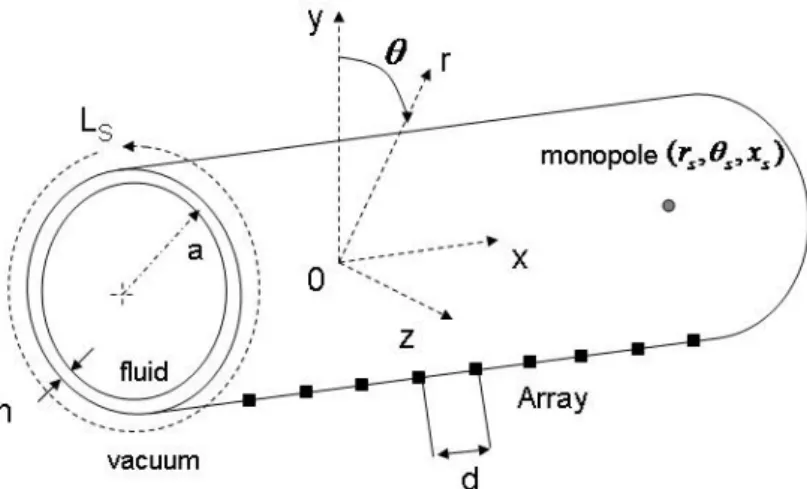
An infinite thin cylindrical shell (representing the external shell of the steam generator) filled with a heavy fluid (i.e. liquid sodium) is excited by an acoustic monopole located inside the fluid at the position s of coordinates(𝑟𝑠, 𝜃𝑠, 𝑥𝑠), as it is shown in Figure 1.
5
Figure 1. Representation of the problem in cylindrical coordinates.
For simplicity reason, the fluid is at rest and the inner structures of the steam generator featuring a bundle of identical parallel tubes surrounded by sodium and filled by water or steam is not taking into account in the model. In a steam generator the fluid flows at low Mach numbers such that it is possible to disregard the convection effect. In a real situation, however, different types of equipment (hydraulic pumps, control vanes) and some turbulence in the fluid maygenerate a strong background noise. In some situations, the noise generated by the monopole may be smothered by the background noise. It would then be difficult to detect and to locate the monopole. In order to highlight the monopole effect compared with the background noise, i.e. to increase the signal-to-noise ratio (SNR), an array of sensors is used to measure the radial vibration velocities of the shell and to feed the beamforming process.
2.2. Beamforming principle
In following developments, a harmonic monopole source pulsating at the angular frequency 𝜔 is taken into consideration and the time dependence term 𝑒−𝑖𝜔𝑡 will be omitted. A broadband
source must be considered in order to extend the harmonic beamforming to a broadband process. A Fourier transform can be used to decompose the signal into discrete frequencies. The harmonic beamforming can be then applied sequentially to each frequency components in turn.
A linear array composed of 𝑁 sensors regularely spaced of a distance 𝑑 and spread over the cylinder along the axial direction is considered. 𝑉̂⃗ 𝑠 represents the radial vibration velocity
6
vector of the fluid-filled shell due to the monopole source whose ith component 𝑣̂𝑠𝑖
corresponds to the vibration velocity measured by the ith sensor of the array (𝑖 = 1 … 𝑁). The Cross Spectrum Densities (CSD) between each couple of sensors is noted in matrix form, given by:
Γ𝑠 = 𝜎𝑠𝑉⃗ 𝑠𝑉⃗ 𝑠†, (1)
where 𝑉⃗ 𝑠. is the normalised vibration velocity vector such that its maximum value is equal to 1, and 𝜎𝑠 is the Auto Spectrum Density (ASD) of the reference sensor (i.e. the sensor with the
highest ASD). 𝑉⃗ 𝑠† is the Hermitian conjugate of the vector 𝑉⃗ 𝑠. Similarly, the background noise
signal may be defined by its CSD matrix:
Γ𝐵𝑔 = 𝜎𝐵𝑔𝐽𝐵𝑔, (2)
where 𝐽𝐵𝑔 represents the normalised CSD matrix of vibration velocities due to the background noise and 𝜎𝐵𝑔 is the ASD of the background noise on the reference sensor. A simple model of background noise (spatially uncorrelated) is considered in this paper. In this case, 𝐽𝐵𝑔is the unit matrix 𝐼𝑁. More complex models can be found in the literature; for instance, different
formulations for the cross-spectrum matrix JBg have been developed for plane structures
excited by a turbulent boundary layer [18], [19].
One assumes that the monopole and the background noise sources are uncorrelated. The total CSD matrix Γ can be then expressed as:
Γ = Γ𝑠+ Γ𝐵𝑔. (3)
The beamforming technique consists in applying a spatial filter to signals of array sensors. The steering vector noted 𝐹 𝑘 characterises the spatial filter applied to the measured signal when the source to detect is supposed to be located at the point k of coordinates (𝑟𝑘, 𝜃𝑘, 𝑥𝑘) in the detection space. The output of the beamforming treatment is a scalar value expressed by:
𝑌𝑘 = 𝐹 𝑘†Γ𝐹 𝑘 . (4)
By introducing (1-3) in (4), the following expression is obtained:
7
Where 𝐷𝑘 is called the directivity function (or ambiguity function) at the point 𝑘 in question.
It is expressed by:
𝐷𝑘 = 𝐹 𝑘†𝑉⃗ 𝑘. 𝑉⃗ 𝑘†𝐹 = |𝐹 𝑘†. 𝑉⃗ 𝑘|2. (6)
The directivity function characterises the ability of the array to locate the source in the detection space.
The efficiency of the beamforming to reject noise is usually defined by its gain 𝐺, expressed as the ratio of the SNR after the beamforming treatment over the SNR on the reference sensor (i.e. 𝜎𝑠/𝜎𝐵𝑔). With the present notation, it is given by:
𝐺 = 𝐷𝑠 𝐹 𝑠†𝐽𝐵𝑔𝐹⃗⃗⃗ 𝑠
, (7)
where 𝐷𝑠 and 𝐹 𝑠represent the directivity function and the steering vector corresponding to the effective position s of the monopole. Eq. (7) shows that the gain can be improved by
maximising 𝐷𝑠 and/or by minimising the filtered background noise 𝐹 𝑠†𝐽𝐵𝑔⃗⃗⃗ . 𝐹𝑠
In practical applications, the background noise is partially or totally unknown, hence, the easier way to improve the gain is to maximize 𝐷𝑠. This condition implies that the scalar product |𝐹 𝑘†. 𝑉⃗ 𝑘|2 is maximal when 𝑘 = 𝑠 which implies that the steering vector must be expressed by:
𝐹 𝑘 = 𝑉⃗ 𝑘
∗
||𝑉⃗ 𝑘||
, (8)
where 𝑉⃗ 𝑘 is the vibration velocity vector of the shell excited by a monopole located at position
k in the detection space.
In order to estimate the steering vector from Eq. (8), the vibration velocity vector must be known for each possible position of the monopole in the detection space. This corresponds to the transfer functions between all the possible positions of the monopole in the detection space and the positions of the array sensors. In practice, measuring these transfer functions may be difficult. Another method consists in calculating them by using a numerical model. In the present paper, a fluid-filled cylindrical infinite shell model is first used to perform
8
3 – Vibro-acoustic modelling of the system
The model described in this section is used to calculate numerically the vibration velocity field on the shell due to a monopole in the internal fluid. These results are used in a first step to calculate the steering vectors of the beamforming treatment and, in a second step, to perform virtual experiments to assess the efficiency of the method.
The problem shown in Figure 1 is considered. The cylindrical steel shell of radius, 𝑎, is
assumed to have an infinite length and a constant thickness, ℎ.𝜌, 𝐸 and 𝜈 are the mass density, the Young’s modulus, and the Poisson’s ratio of steel, respectively. The shell is filled with liquid sodium supposed at rest. 𝜌0 and 𝑐0 are respectively the mass density of the sodium and the acoustic wave phase velocity in the sodium. The effect of the fluid convection is not considered. The behaviour of the shell may be represented by Flügge’s equations of motion, while the fluid behaviour may be represented by Helmholtz’s equation with Somerfield’s conditions at infinity. This problem was solved by Fuller [20] which studied the mobility of the shell and the energy ratio transiting threw the acoustic and the structural subsystems as a function of the frequency, radial and axial monopole positions inside the fluid. The problem involves expressing the original equations in the wavenumber domain by applying the space-Fourier transform defined by Eq. (9), which takes into account that the function 𝑓(𝑥, 𝜃) is 2𝜋 periodic along 𝜃: 𝑓(𝑥, 𝜃) → 𝑓̃(𝑘𝑥, 𝑛) = ∫ ∫ 𝑓(𝑥, 𝜃)𝑒𝑘𝑥𝑥+𝑛𝜃𝑑𝜃𝑑𝑥 2𝜋 0 +∞ −∞ , (9)
where 𝑘𝑥 is the axial wavenumber and n the circumferential order (𝑛 𝜖 ℕ).
A linear system of equations is then obtained (see [20] for details). The unknowns of this system are the shell velocities expressed in the wavenumber space which can be easily deduced by inverting the system.
Finally, the radial velocity of the shell in the wavenumber domain is given by:
𝑣̃(𝑘𝑥, 𝑛) = 2𝑞𝑠(−𝑖𝜔)𝐽𝑛(𝑘𝑟𝑟𝑠)𝑒𝑛𝜃𝑠+𝑘𝑥𝑥𝑠 𝑘𝑟𝑎𝐽𝑛′(𝑘𝑟𝑎) (𝑙11′ 𝑙 22′ − 𝑙22′ 2) det |𝐿′| , (10)
9 where:
- 𝑞𝑠 is the strength of the monopole source,
- 𝐽𝑛 is the nth order Bessel function,
- 𝐿′ is the space-Fourier transform of Flügge’s operator taking into account the fluid
loading term,
- 𝐿′𝑖𝑗 corresponds to (𝑖, 𝑗) element of the matrix 𝐿′,
- 𝑘𝑟 is the radial wavenumber which is related to 𝑘𝑥 by:
𝑘𝑟 = ±(𝑘02− 𝑘
𝑥2)1/2 , (11)
where 𝑘0 = 𝜔/𝑐0 is the acoustic wavenumber. The matrix 𝐿′ depends on shell and fluid
parameters (see the expressions in [20]). The radial velocity 𝑣̃ can then be calculated analytically with Eq. (10). Fuller [20] estimated numerically the poles of Eq. (10) to deduce the radial velocity 𝑣 in the physical space. An alternative method consists in applying an inverse discrete Fourier transform to Eq. (10) after windowing and sampling the wavenumber space (see [21]): 𝑣(𝑥, 𝜃) = ∑ 𝑒𝑖𝑛𝜃 𝑁̅ 𝑛=−𝑁̅ ∑ 𝑣̃ 𝐾̅ 𝑘=−𝐾̅ (𝑘𝛿𝑘𝑥, 𝑛)𝑒𝑖𝑘𝛿𝑘𝑥𝑥𝛿𝑘𝑥. (12)
The truncation indices 𝐾̅, 𝑁̅ and the sampling wavenumber mesh 𝛿𝑘𝑥 can be evaluated from the physical parameters of the shell by using the criteria defined in [21] (i.e. eq. (26) and (27) in [21]). The radial vibration field of the shell can then be quickly calculated by using Eq. (10) and a Fast Fourier Transform (FFT) algorithm for calculating Eq. (12) with MATLAB.
Considering the calculation process when the monopole is located at a point 𝑘 makes possible the evaluation of steering vectors with Eq. (8) for each position of the detection space. In practice, it is not necessary to calculate steering vectors in real time. They can be predefined. Only the matrix-vector product of Eq. (4) should be calculated in pseudo-real time.
Experimentally, steering vectors can be defined from measurements in a preliminary stage of the use of the beamforming. It is then necessary to move an acoustic source (for example, a hydrophone) in the detection space and to save for each position, the signals measured by the array. Another possibility is to use a numerical model to evaluate steering vectors. In this
10
case, the model must be sufficiently accurate to capture the main physical behaviour of the considered system.
11
4 – Results
In this section, numerical results of beamforming are presented for a cylindrical fluid-filled shell with a radius 𝑎 = 445 𝑚𝑚 and a thickness ℎ = 28 𝑚𝑚. The dimensions of the
cylindrical shell have been defined in accordance to basic design data of a new modular steam generator energy conversion system. These values correspond to the design of a straight-tube bundle steam generator. The fluid medium has acoustical properties of liquid sodium at 500°C (i.e. 𝜌0 = 830 𝑘𝑔/𝑚−3, 𝑐0 = 2300𝑚/𝑠−1) and the shell is made of stainless steel (i.e.
𝜌0 = 7800 𝑘𝑔/𝑚−3, 𝐸 = 2.03.1011 𝑃𝑎, 𝜈 = 0.3). In the following, numerical results are
obtained by proceeding the beamforming treatment throw a linear array of 10 m length composed of 𝑁 sensors spread on the axial direction as shown in Figure 1. The ith sensor of
the array is located at the positions of coordinates (𝑟𝑖 = 𝑎, 𝜃𝑖 = 0°, 𝑥𝑖 = −5 + (𝑖 − 1)𝑑). The CSD matrix Γ𝑠 of resulting radial shell velocities is calculated with Eq. (1). The steering vector 𝐹 𝑘 is calculated for each position 𝑘 of the detection space by using Eq. (8), Eq. (10) and Eq (12). Values of the directivity function on the detection space are calculated using Eq. (6) and the array gain is calculated using Eq. (7). A spatially incoherent background noise is considered (i.e.𝐽𝐵𝑔 = 𝐼𝑁, an identity matrix). Then, the array gain is equal to the directivity
function 𝐷𝑠 when the array focuses on position s (see Eq. (7-8)).
This simple array pattern is considered to study the possibility of improving the SNR and the influence of different parameters on the monopole detection and localisation. In practical applications, a more complex array pattern may be considered in order to optimise the final detection ratio.
In order to include some energy dissipation in the model, damping factors are introduced into the shell material (fluid properties respectively) by assigning a complex value with a loss factor 𝜂𝑠 (𝜂𝑓 respectively) to the elastic modulus 𝐸 (acoustic phase velocity 𝑐0 respectively).
In practice, evaluating structural and acoustic damping loss factors is difficult since they vary with many parameters [22]. Steel alloy damping loss factors are generally around 10−3 [23].
The presence of structures inside the steam generator (tube bundle, spacing grids) and insulation material around it may significantly increase this value. In the following, it is assumed that the structural damping loss factor 𝜂𝑠 is equal to 10−2. Similarly, the presence of
internal structures, residual hydrogen and argon must be taken into consideration to estimate the dynamic loss factor in liquid sodium. In the following, this value has been set at
12
𝜂𝑓= 10−3. Nevertheless, a variation of these parameters changes the energy distribution
between both the structural and the acoustic media. The effect of such fluctuations on the performance of the monopole detection with the present technique is presented in section 4.2.3
4.1 Vibration field analysis in the wavenumber space
First, an acoustic monopole is considered to be located in the fluid at the position s of
coordinates (𝑟𝑠 = 0.3 𝑚, 𝜃𝑠 = 0°, 𝑥𝑠 = 0 𝑚). Equation (10) provides a wave decomposition of the radial velocity field of the shell for a given frequency. By analysing this decomposition, the axial wavenumbers of the most significant waves can be extracted. Here, waves are assumed to be significant if their amplitudes normalised to the highest wave amplitude (at the given frequency) are greater than -10 dB. Wavelengths corresponding to these significant waves can then be easily deduced.
Axial wavenumbers of significant waves, noted 𝑘𝑚𝑎𝑥, are shown in Figure 2 as a function of the frequency. To better understand this figure, two characteristic wavenumbers are also plotted:
- the first one is the acoustic wavenumber 𝑘0 which characterises the acoustic
propagation in the internal fluid medium;
- the second is the flexural wavenumber 𝑘𝑓 of an infinite plate equivalent to the shell
(same material and thickness) in which the mass added by the fluid is considered. This wavenumber is defined in reference [21].
13
Figure 2. Axial wavenumbers of normalised radial velocity amplitudes considering all mode numbers n for a monopole located at position s (𝑟𝑠 = 0.3 𝑚, 𝜃𝑠 = 0°, 𝑥𝑠 = 0 𝑚;
, [𝐿𝑚𝑎𝑥𝑤 − 3𝑑𝐵, 𝐿 𝑤 𝑚𝑎𝑥] ; ,[𝐿 𝑤 𝑚𝑎𝑥− 5𝑑𝐵, 𝐿 𝑤 𝑚𝑎𝑥− 3𝑑𝐵] ; ,[𝐿 𝑤 𝑚𝑎𝑥− 10𝑑𝐵, 𝐿 𝑤 𝑚𝑎𝑥 − 5𝑑𝐵].
(Dashed line) acoustic wavenumber (𝑘0); (dash-dotted line) flexural wavenumber of an
equivalent plate (𝑘𝑓).
For frequencies above the ring frequency of the shell, it is well known that the curvature effect of the shell is negligible and radial motions of the shell approximate the flexural motions of a plate. For frequencies below the ring frequency, the curvature of the shell stiffens the shell in the axial direction and its dominant axial wavenumber should be lower than 𝑘𝑓.
The considered system is composed of two parts: the elastic shell and the fluid medium. As one considers a heavy fluid (i.e. sodium), the interaction between these two parts is strong. Then, the dominant waves can propagate both, in the shell and in the fluid medium. This strong coupling leads to a shift of their positions in the wavenumber spaces compared to a wave propagating in the shell or in the fluid medium only. However, as characteristic wavenumbers of these two parts are significantly different, one can identify waves mainly influenced by the shell behaviour and others mainly influenced by the fluid behaviour. The
14
first types of waves are called here quasi-structural waves whereas the second ones are called quasi-acoustic waves.
In Figure 2, three frequency domains can be identified:
- At low frequencies (𝑓 < 1300 Hz), the radial velocity field of the shell is mainly distributed on axial wavenumbers higher than the acoustic wavenumber 𝑘0. Their
values increase with the frequency and seem to converge to the flexural wavenumber 𝑘𝑓. The vibration behaviour of the shell coupled to the internal fluid is dominated by
the shell behaviour in this frequency domain. Quasi-structural waves propagate in this frequency domain which is called the structural predominance domain.
- In the intermediary frequency domain (1300 Hz < 𝑓 < 1800 Hz), vibrations are supported by axial wavenumbers located close to the flexural wavenumber 𝑘𝑓 and below the acoustic wavenumber. In this domain, the acoustic behaviour seems to get progressively stronger than the structural behaviour. This frequency domain is called the transitional domain.
- At higher frequencies (𝑓 > 1800 Hz), the radial velocity field is mainly supported by wavenumbers located below the acoustic wavenumber 𝑘0, corresponding to high wavelengths. The vibration behaviour of the shell coupled to the internal fluid is dominated by the behaviour of the internal fluid. Quasi-acoustic waves propagate in this frequency domain which is called the acoustic predominance domain.
It is important to note that this
4.2 Detecting and locating the monopole
In this section, experiments are performed numerically by using the model described in section 3. An acoustic monopole is located at the position s of coordinates (rs=0.3 m, s=0°,
xs=3 m).
4.2.1 Influence of the number of sensors
In this section, the influence of the number of sensors constituting the array on performances of the beamforming is studied. Values of the directivity function are represented in Figure 3 in the axial plane 𝜃 = 𝜃𝑠 and in the circumferential plane 𝑥 = 𝑥𝑠 which cut together in the radial
15
of 1 kHz which belongs to the structural predominance domain according to results shown in Figure 2.
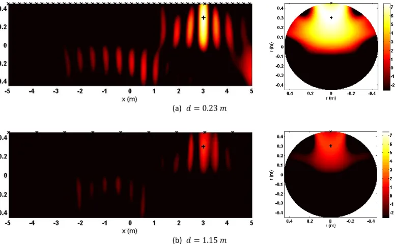
In Figure 3.a, the distance d is equal to the half flexural wavenumber 𝜆𝑓/2 = 𝜋/𝑘𝑓 whereas it is equal to the half acoustic wavelength 𝜆0/2 = 𝜋/𝑘0 in Figure 3.b
(a) 𝑑 = 0.23 𝑚
(b) 𝑑 = 1.15 𝑚
Figure 3. Directivity function (dB) in the plane 𝜃 = 𝜃𝑠 and in the plane 𝑥 = 𝑥𝑠. Monopole
located at the position 𝒔 (𝑟𝑠 = 0.3 𝑚, 𝜃𝑠 = 0°, 𝑥𝑠 = 3 𝑚) (represented by a black symbol +) pulsating at the frequency 𝑓 = 1 𝑘𝐻𝑧; space between sensors (represented by black symbols ×) (a) 𝑑 = 𝜆𝑓
2 = 0.23𝑚, (b) 𝑑 = 𝜆𝑓
2 = 1.15𝑚.
In this figure, sensors positions are represented by black symbols × whereas the monopole position s is represented by a black symbol +. The maximum value of the directivity function, 𝐷𝑠 is located at the position s. The domain around this position, where the directivity function ranges are in the interval [𝐷𝑠-3 dB; 𝐷𝑠], is called the primary lobe. Other lobes on which the directivity function can reach high values (but still inferior to 𝐷𝑠) are called side lobes. According to Figure 2 and Shannon’s criterion for spatial sampling in the axial direction, a space 𝑑 = 𝜆𝑓/2 should be small enough to ensure a good spatial sampling of smaller
16
wavelengths (or higher wavenumbers) constituting the vibration field of the system. In consequence, increasing the number of sensors (by decreasing 𝑑) will increase the array gain and the amplitude of side-lobes in proportion but will not increase the accuracy of the
localisation. As a contrary, increasing the distance d above 𝜆𝑓/2 may lead to aliasing effects
and a decrease of beamforming performances. In Figure 3.b, the value of 𝑑 has increased to the value of the half acoustic wavelength 𝜆0/2 which is higher than wavelengths of
importance according to Figure 2. Then, two negative effects can be noticed. First, the whole values of the directivity function are decreased compared to those presented in Figure 3.a. This effect is due to the diminution of the number of sensors participating to the
beamforming.
The second effect is an increase of the number of side-lobes and of their amplitude (relatively to the amplitude of the primary lobe). In consequence, the localisation is rendered difficult even if the maximum value of the directivity function is still located exactly at the monopole position. This second effect can be explained by the spatial sub-sampling of the vibration field due to the high value of 𝑑.
The effect of a diminution of the number of sensors is presented in more details in Figure 4. In this figure, the monopole is centred on the array at the position s of coordinates
𝑟𝑠 = 0.3𝑚, 𝜃𝑠 = 0°, 𝑥𝑠 = 0𝑚). The length and the position of the array remains unchanged but the distance d between each sensor increases from 0.1 m (99 sensors) to 10 m (2 sensors). In order to represents results in both acoustic and structural predominance domains, four frequencies are considered: 500 Hz, 1 kHz, 3 kHz and 5 kHz.
Values of the array gain are represented in Figure 4.a against the distance d and for these four frequencies. A theoretical result, given by Urick in the case of a linear array composed of regularly spaced sensors measuring pressure variations in an acoustic medium in which a plane wave propagates, is also plotted. In this case, all sensors measure the same amplitude so they participates to the beamforming in equal proportion and the array gain is the maximum which can be expected. The array gain is then only dependent of the number of sensors and its value is simply equal 10 log10(𝑁) [10]. The present case is however different in many points
to the one studied by Urick but it is pertinent to take this theoretical result as a reference. For the four frequencies considered, the array gain varies around a mean value which is quasi-logarithmic with the number of sensors and always smaller than the maximum value of
Urick’s law. These fluctuations are due to the position of the source in function of the distance
17
value or to a low value of the gain respectively. Despite the strong differences between the present case and Urick’s case, the logarithmic evolution of the gain is observed and increasing the distance d seems to have no particular impact on the value of the gain expect the one related to diminution of the number of sensors.
Figure 4. (a) Array gain (dB) against sensor spacing, blue dashed line: Urick’s law; (b) Relative amplitude attenuation between the primary lobe and the first side-lobe (dB) against sensors spacing 𝒅; monopole position 𝒔 (𝒓𝒔 = 𝟎. 𝟑𝒎, 𝜽𝒔 = 𝟎°, 𝒙𝒔 = 𝟎 𝒎) pulsating at (red
line) 5 kHz, (blue line) 3 kHz, (black line) 1 kHz and (green line) 500 Hz.
Figure 4.b represents the difference between the amplitude of the primary lobe and the higher side lobe (which is noted Δ𝐿) in function of the distance d and for the four frequencies considered previously. This value is an indicator of the performance of the localisation of the monopole in the detection space. Two behaviours can be observed. First, Δ𝐿 is quasi-linear whereas d increases. In this domain, the localisation is the best which can be expected with this array pattern. Increasing the number of sensors (by decreasing d) will increases the whole values of the directivity function. In consequence, the gain will increase but not the
performance of the localisation. Above a critical value of d (noted 𝑑𝑐), Δ𝐿 begins to fluctuate
10-1 100 101 0 5 10 15 20
Distance between sensors (m)
G ( d B , re f. 1 )
(a) Array Gain
10-1 100 101 0 2 4 6 8 10
Distance between sensors (m)
L ( d B , re f. G )
(b) Relative amplitude attenuation of side-lobe
1 kHz 5 kHz 3 kHz 0.5 kHz Urick's theory f 1kHz/2 0 5kHz/2 0 3kHz /2 f 0.5kHz/2
18
around a value which decreases progressively to 0. Fluctuations are due to the relative
position of the source and of the sensors. This effect was explained previously in the analysis of the Figure 4.a. The diminution of the mean value of Δ𝐿 characterises the degradation of the monopole localisation in the detection space. The critical value 𝑑𝑐 depends on the frequency considered and corresponds to the half higher wavelength of importance highlighted in section 4.1. At 500 Hz and at 1000 Hz, one can see that 𝑑𝑐 ≈ 𝜆𝑓/2 whereas 𝑑𝑐 ≈ 𝜆0/2 at 3000 Hz and at 5000 Hz. This result is coherent with the existence of an acoustic and a structural predominance domain highlighted previously and confirms that a spatial Shannon’s criteria should be respected for maximising the localisation of the monopole. Nevertheless, the localisation can be possible (and sometimes more accurate) when the distance 𝑑 > 𝑑𝑐 because of fluctuations of the gain and of Δ𝐿 but the behaviour of these values in this domain may be difficultly predictable. For this reason, one recommends to respect the spatial
Shannon’s criterion corresponding to the considered frequency and to define the number of sensors in function of the expected gain.
4.2.2 Influence of the radial monopole position
As discussed in reference [20], the vibrational energy between the shell and fluid media depends on the radial monopole position. When the monopole is located close to the shell (far from the shell respectively), the vibrational energy is predominantly in the shell (in the fluid respectively) which may impact detection by the array. This section investigates the influence of the radial monopole position on detection. A sensor spacing 𝑑 = 0.2 m is taken into account to ensure that spatial Shannon’s criterion is met both at 1 kHz and 5 kHz. The corresponding number of sensors is therefore 51.
The array gain is plotted in figure 5.a as a function of the radial position 𝑟𝑠 of the monopole
19
Figure 5. Variation of the gain (dB) (a), the reference radial velocity (dB) (b) and the
normalised mean deviation (dB) (c), at 1 kHz (dash line) and 5 kHz (solid line), against radial monopole position 𝑟𝑠; 𝑑 = 0.2𝑚.
It can be seen that the gain varies significantly as a function of 𝑟𝑠 and that this variation depends on the frequency. Some significant peaks appear, particularly at 5 kHz. It is necessary to analyse the signals measured (virtually) by the array sensors in order to understand these phenomena. The following is plotted:
- figure 5.b shows the highest radial velocity amplitude measured by the reference sensor for each radial monopole position,
- figure 5.c shows the normalised mean deviation (NMD) of the array signals which is defined with analogy to the standard deviation by:
𝑁𝑀𝐷 = √1 𝑁∑ ( |𝑣𝑖| − |𝑣𝑟𝑒𝑓| |𝑣𝑟𝑒𝑓| ) 𝑁 𝑖=1 2 , (13)
20
where 𝑣𝑖 and 𝑣𝑟𝑒𝑓 are the radial velocity at the sensor i and at the reference sensor of the
array, respectively.
A small NMD corresponds to a low spatial variation of the signals measured by the array sensors. It indicates that the vibration field measured by the sensors is almost homogeneous and a large number of sensors effectively contribute to beamforming. On the contrary, a high
NMD indicates a strong axial decay in the vibration field measured by the sensors. In this
case, few sensors effectively contribute to beamforming, which can lead to poor efficiency in the array treatment.
It can be seen in Figure 5.b that positions of gain peaks correspond to the positions of
minimum amplitudes measured by the reference sensor. This indicates that the array treatment is most efficient for specific positions for which it would have been difficult to detect the source with only one sensor. As the vibration measured by the reference sensor is low for these specific positions, it can be concluded that the monopole source weakly excites the system for these positions which certainly correspond to nodal points of the global modes of the fluid loaded shell. Moreover, Figure 5.c shows that the NMD is also lower for these positions than for other ones. This explains why the highest array gain values are obtained for these specific positions. In these cases of low NMD, the vibration field measured by the sensors is almost homogeneous, a large number of sensors contribute to beamforming and the array gain is “high”. In the other cases, only sensors located close to the reference contribute to beamforming and the gain is small.
4.2.3 Influence of damping loss factors
In order to take some energy dissipation into account in the system, damping loss factors for the shell and the fluid were introduced into the model through a complex Young’s modulus and the acoustic phase velocity. It is, however, difficult to estimate the real value of these parameters for the SGU in question. The vibrational energy distribution between the shell and the fluid can depend on these parameters. In this section, a parametric study is done to assess the impact of acoustic and structural damping loss factors on the detection performance.
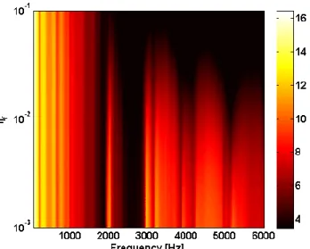
The array gain is shown in Figure 6 as a function of the fluid damping loss factor, increasing from 0.1% to 10% and the frequency increasing from 50 Hz to 6 kHz. The structural damping loss factor is equal to 1% and the monopole source is located at the position s of coordinates (𝑟𝑠 = 0.3𝑚, 𝜃𝑠 = 0°, 𝑥𝑠 = 3𝑚).
21
Figure 6. Array gain (dB) in function of the frequency and the fluid damping loss factor. Structural damping loss factor of 1 % (𝜂𝑠 = 0.001). Monopole located at position s (𝑟𝑠 = 0.3𝑚, 𝜃𝑠 = 0°, 𝑥𝑠 = 3𝑚).𝑑 = 0.2𝑚.
The gain reaches its highest values in the low frequency domain corresponding to the
structural predominance domain. As one saw in section 4.1, quasi-structural waves dominate at these frequencies. The vibrational behaviour of the fluid filled shell is dominated by the dynamic behaviour of the shell and the influence of the fluid damping is then negligible at these frequencies. Consequently, an increase of the acoustic damping factor barely impacts the performance of the detection as observed on Figure 6.
In the acoustic predominance domain, significant values are observed for frequencies corresponding to a propagation of dominant waves having small axial wavenumbers 𝑘𝑥𝑚𝑎𝑥
(see Figure 2). These frequencies correspond to the cut-on frequencies for the propagation of quasi-acoustic waves (for different circumferential orders). Above these cut-on frequencies, wavenumbers 𝑘𝑥𝑚𝑎𝑥 increase and the gain value decreases. In this frequency domain, the gain
falls sharply and reaches values below 6 dB when the acoustic damping factor increases above a critical value (around 3% at 2 kHz). This can be explained by the fact that the vibrational amplitude measured by the sensors located far from the reference one are more and more attenuated because of the spatial decay of the quasi-acoustic waves due to the acoustic damping effect. Therefore, less and less sensors participate effectively to the beamforming when the acoustic damping increases. In consequence, the gain decreases as
22
observed on Figure 6. Then, increasing the acoustic damping factor reduces the performance of the detection at this frequency.
The fluid damping plays a role in the acoustic predominance domain, only. In this domain, the quasi-acoustic waves can be strongly attenuated by the damping effect, causing a dramatic fall of the beamforming performance. The critical value of the damping loss factor for which the gain falls depends on the frequency. For the case considered on Figure 6, this value seems relatively high (i.e. around 3% at 2 kHz).
Now, the array gain is shown in Figure 7 as a function of the structural damping loss factor, increasing from 0.1% to 10% and the frequency, increasing from 50 Hz to 6 kHz. The acoustic damping loss factor is equal to 0.1%. The monopole position is unchanged.
Figure 7. Array gain (dB) in function of the frequency and the structural damping loss factor. Fluid damping loss factor of 0.1 % (𝜂𝑓= 0.001). Monopole located at position s (𝑟𝑠 = 0.3𝑚, 𝜃𝑠 = 0°, 𝑥𝑠 = 3𝑚); 𝑑 = 0.2𝑚.
As it was observed in Figure 6, the gain reaches its highest values in the structural
predominance domain regardless the structural damping factor. Significant values are also observed in the acoustic predominance domain when the dominant axial wavenumber 𝑘𝑥𝑚𝑎𝑥 is
small. Contrary to one could observe in the acoustic predominance domain when the acoustic damping increases, the gain is weakly impacted by an increase of the structural damping in both frequency domains.
23
In conclusion, the performance of the beamforming is weakly impacted by acoustic and structural damping factors in the low frequency region for which quasi-structural waves dominate the vibratory field of the shell. On the contrary, the gain is sharply reduced in the acoustic predominance domain when the acoustic damping increases. However, for a fluid lightly damped, the array gain remains satisfactory.
4.2.4 Impact of fluid properties modifications
During the SGU operation, small quantities of argon or some residual hydrogen can be present in the liquid sodium which can weakly affect the acoustic medium by changing locally its physical properties [24]. In consequence, beamforming performances might fluctuate if steering vectors are calculated using transfer functions measured before the leak. One analyzes the evolution of the array gain whereas steering vectors are calculated
considering acoustic celerity and acoustic density values higher than those used in the model. It is however difficult to estimate how these parameters fluctuate during the SGU operation. Considering the relatively small quantity of residual gas in the liquid sodium of the SGU, we have assumed that these modifications were smaller than 5%. The consequences of such variations on the beamforming performances in these structural and acoustic predominance domains are discussed in this section.
Figure 8 shows the evolution of the array gain whereas steering vectors are calculated
considering acoustic density and acoustic celerity values equal (black plain lines), and higher by 1% (black dotted lines) or by 5% (black dashed lines) than those used in the model.
24
Figure 8. Evolution of the array gain (dB) against the frequency whereas steering vectors are calculated with an overestimation of (black plain lines) 0%, (black dotted lines) 1% and (black dashed lines) 5% on (a) the acoustic mass density and (b) on the acoustic celerity; acoustic monopole located at the position 𝒔 (𝒓𝒔 = 𝟎. 𝟑 𝒎, 𝜽𝒔 = 𝟎°, 𝒙𝒔 = 𝟎 𝒎); d = 0.1 m. On these two graphs, two frequency domains corresponding to the structural and acoustic predominance domains can be identified. In the structural predominance domain, the variation of the acoustic mass density and the acoustic celerity has a negligible influence on the array gain. The method is then not significantly disturbed in this frequency range. When the
acoustic mass density is overestimated the gain seems to be not disturbed until around 3 kHz, except in a frequency range comprised between 2.2 Hz and 2.4 kHz where a dropping of about 5 dB is observed. Above 3 Hz, the gain decreases from its nominal value whereas the acoustic mass density is overestimated, and this effect is accentuated when this overestimation increases.
In the acoustic predominance domain, starting below 1.9 Hz, the gain falls sharply when the acoustic celerity is overestimated by 1% and this behavior is accentuated when it is overestimated by 5%. These results are not surprising because in the structural predominance domain, the wave propagation is dominated by the mechanical behavior of the system which is not impacted by these parameters. On the other hand, in the acoustic predominance domain, the acoustic celerity impacts directly the wave propagation and the phase of signals measured by the array. 0 1000 2000 3000 4000 5000 6000 -20 -10 0 10 20 Frequency (Hz) A rr a y G a in d B 0 1000 2000 3000 4000 5000 6000 -20 -10 0 10 20 Frequency (Hz) A rr a y G a in d B 0 0 + 1% 0 + 5% c 0 c0 + 1% c 0 + 5%
25
Once again, these results prove that the method is more stable in the structural predominance domain than in the acoustic predominance domain because properties of the shell are not supposed to vary during operation.
In conclusion, the performance of the beamforming is weakly impacted by a modification of acoustic properties during a leak in the structural predominance domain. On the contrary, the gain is reduced in the acoustic predominance domain when a deviation of the acoustic mass density and, even more, on the acoustic celerity is considered in the steering vectors
26
5. Mock-up experiment
5.1 Experimental set-up
The experiment presented in this section and in Figure 9 has been done to confirm the
efficiency of the beamforming method which was previously tested with a numerical model in section 4. The SGU shell is a thin cylinder of about 30 m length, connected to a hydraulic loop in which waves can propagate without being reflected, but waves progressing through the shell are reflected at its extremities. For modelling such a system, we assume that an infinite cylinder is more realistic than a finite cylinder. Even if it is idealistic, such a model is useful to represent the propagation of waves in the liquid sodium without reflection and to test the method numerically but it is not pertinent to study the real behavior of the SGU since it does not take into account the presence of axial modes of the shell. Nevertheless, these axial modes are present in the mock-up which, for practical reasons, represents a relatively small section of the SGU, connected to a hydraulic loop with links stiffer than the shell. Axial modes were studied on the empty mock-up previously to the experiment. Steering vectors were not defined using the numerical model which does not describe axial modes. They were calculated from experimental transfer functions in which axial modes are intrinsic. For the conception of SGU, studying the influence of modes of the system on the performances of the beamforming method could be of interest. However, it does not enter into the scope of the present paper.
The mock-up is composed of a cylindrical cylinder made of stainless steel and filled with water. The cylinder consists in a reduced scale of the straight-tube bundle steam generator. The liquid sodium has been replaced by water for convenient and safety reasons. To define the geometric characteristics of the mock-up, we took into account the fact that an effect observed at a certain frequency in the real scale steam generator can be observed at a different frequency in the mock-up because of diameter and internal fluid changes.
The length scale ratio 𝛾𝑓 and the frequency scale ratio 𝛾𝐹 are defined in order to keep the same numbers of acoustic wavelength along the radius of the steam generator at the real frequency,𝑓 and in the mock-up at the experimental frequency, 𝑓′. Then we consider the
relation:
27 𝛾𝐿 =
𝑐0
𝑐0′𝛾 𝐹,
where c0 and c0’ are the acoustic phase velocity in the sodium at f and in the water at 𝑓′,
respectively and 𝛾𝐹 = 𝑓′/𝑓. Setting the cylinder diameter of the mock-up at 0.219 m and the
maximum experimental frequency at 15 kHz, we obtain F 2.4 and L 3.6 that fixed the
length of the cylinder to 306 cm and its thickness to 0.82 cm.
(a) (b)
(c)
Figure 9. Mock-up: (a), schema of the water filled cylinder with the array and the different positions of excitation; (b), design of the acoustic excitation device. (c) Picture of the mock-up with the array on the top and source excitation device on the bottom of the cylinder.
In order to simulate the noise generated by a sodium leak, a specified device has been designed as shown on Figure 9.b. It allows us to put a hydrophone B&K 8103 at different radius position. It is used as an acoustic emitter (i.e. projector). The radial positions considered in the detection space are – 64 mm, - 2 mm, 47 mm and 88 mm (defined in the cylindrical coordinate system of figure 1).
28
The acoustic excitation system can be inserted in 6 different holes spread over along the cylinder at 6 different axial positions. All in all, the system can be excited by the hydrophone at 24 positions represented by green squares in Figure 9. The hydrophone is excited by a harmonic signal. The amplitude and the frequency of the signal can be controlled.
The background noise can be controlled by maintaining the flow regime at a given speed of pump. The maximum water flow velocity is 2.1 m/s (i.e. 70 l/s).
A linear array of 1 m length, composed of 50 accelerometers Kistler 8704B50 regularly spaced, is used to sample the radial vibration field of the water filled cylinder.
We plotted the diagram of the axial wavenumbers of the predominant waves for the mock-up cylinder (as for figure 2) and we checked that the sensor spacing (i.e. 2 cm) is large enough to respect the spatial Shannon criterion whatever the frequency below 15 kHz.
The signals from the accelerometers are recorded with a PULSE B&K acquisition system. Applying a fast Fourier transform (FFT) to the signals measured by the 50 accelerometers gives us the spectral acceleration at each sensor position. Spectral accelerations measured by all the accelerometers of the array constitute a spatial sample of the radial acceleration field on the structure, at each frequency.
The determination of the steering vectors which are used to filter the signal measured by the array of sensors is of prime importance. This can be done using a numerical model having a high degree of reliability or by measuring radial accelerations of the shell experimentally for different positions of the source. The second solution has been employed here. It necessitates a preliminary “learning phase” to create a base of steering vectors. When the fluid is at rest and the background noise is as low as possible, the measurements achieved with the emitter at a given position, are used to define the steering vector for the given position (with Eq. (8)). This operation has been repeated for each of the 24 possible positions (symbolised by green squares in figure 9). In order to enlarge the detection space, a plane of symmetry has been supposed at the middle of the array. It allows us defining eight supplementary positions in the detection space as illustrated in figure 9 with red squares. The steering vectors for these positions are approximated from the ones of the symmetric positions. Because steering vectors are estimated using experimental transfer functions, it is important to note that they take into account all the paths of energy propagation from the piezoelectric device of the hydrophone to each accelerometer of the array. This includes both the acoustic propagation in
29
interaction with the structure and the direct wave propagation through the excitation device and the cylindrical shell. It is however difficult to measure the contribution of this second path, which is ideally not expected. However, the difference of dynamic rigidity between a 8.2 mm thick shell and the 1 mm thick support of the hydrophone, allows to neglect this second path.
5.2 Experimental Results
In this section, performances of the method are studied in function of several parameters, such as the initial signal-to-noise ratio on the reference sensor, the frequency of the signal emitted by the hydrophone and the water flow speed.
5.2.1 Spatial Coherences induced by the Source and the Background Noise
From its principle, the beamforming method is efficient when the signal to detect is spatially coherent whereas the background noise is spatially incoherent. The validity of these assumptions is investigated in this section.
The hydrophone is first located in water at position xs = 755 mm and rs = 47 mm. It
emits a harmonic signal at 6 kHz and water is at rest in the mock-up. The background noise is as low as possible. It is constituted of the electronic noise of the accelerometers and of the ambient noise in the experimental building. Vibrations are recorded during 5 s by the 50 accelerometers simultaneously. The sampling frequency is 32768 Hz. The coherences
between each pair of sensors at this frequency are close to one. Similar results are obtained for every frequencies and hydrophone positions considered in this paper. This allows us to check that the considered hydrophone is able to induce a vibratory field which is completely
spatially coherent.
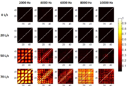
In order to characterize the spatial coherency of the background noise, the same process is achieved when the hydrophone is off and the water flows in the mock-up. Four water flow speeds are considered: 0 l/s, 20 l/s, 50 l/s and 70 l/s. The matrices of coherences between each pair of sensors are represented in figure 10 for 5 frequencies.
30
Figure 10. Analysis of the background noise: values of the coherence between each pair of sensors at 2 kHz, 4 kHz, 6 kHz, 8 kHz and 10 kHz, for a fluid flowing at 0 l/s, 20 l/s, 50 l/s and 70 l/s,
When water is at rest, the signals measured correspond to the background noise which is by nature completely incoherent. Then, the matrix of coherences has diagonal terms close to unity and non-diagonal terms close to zero for every frequency. Increasing the water flow speed up to 20 l/s does not make significant changes in the coherence matrix. When the water flows at 50 l/s, the Reynolds number is about 105 and the flow can be considered as turbulent. We observe that the vibrational response of the cylinder is partially spatially coherent at 2 kHz and 4 kHz but remains incoherent at higher frequencies. Thus, the turbulent flow induces significant vibration compared to the background noise only for the lower frequencies. When the flow speed increases up to 70 l/s, the pressure fluctuations due to the turbulent flow induce significant vibrations at all considered frequencies. It results that the vibration field of the cylinder is partially spatially coherent for all these frequencies.
In conclusion, it could be expected that the beamforming treatment will be the more efficient at low flow speeds and/or at high frequencies.
31
5.2.2 Influence of the SNR on the Performance of the Beamforming
The hydrophone, located at the position xs = 755 mm and rs = 47 mm emits a harmonic
signal at 6 kHz. Five experimental configurations in term of background noise and Signal-to-Noise Ratio are considered. In configurations 1 to 3, the water is at rest in the loop and the background noise is the incoherent “ambient noise”. In configurations 4 and 5, the background noise is due to vibrations induced by the turbulent water flow at 70 l/s. Its spatial coherency at 6 kHz is represented in figure 11 Different low SNRs are defined as summarized in table 1. Configurations 1 and 4 correspond to the background noises without a source signal. They are used to analyze the noise rejection by the beamforming.
Configuration N° Background Noise SNR 1 Ambient - ∞ 2 Ambient - 3 dB 3 Ambient 3 dB 4 Turbulent - ∞ 5 Turbulent 10 dB
Table 1. Definition of the experimental configurations
To obtain the low SNR of table 1, the experimental process is decomposed in three steps: The first step consists in measuring the background noise by the array (which will be supposed stationary); in a second step, the projector is excited with a “high” reference voltage,Vref in order to ensure to be well above the background noise. A reference Signal-to-Noise Ratio,
ref
SNR can be evaluated from the previous measurement (on the reference sensor, as defined in section 2). The last step consists in decreasing the input voltage to the value V such that the SNR is given by: 20 log ref ref V SNR SNR V . (15)
32
Eq. (5). Results for each position in the detection space are plotted in figures 11 and 12. The position of the hydrophone is represented by a black circle whereas the position of the accelerometers is represented by black crosses.
Figure 11. Beamforming output values for each position of the detection space at 6 kHz: (a), configuration 1; (b), configuration 2; (c), configuration 3. Position of the projector symbolized with a black circle and positions of the accelerometers symbolized with black crosses.
Result in figure 11.a corresponds to the configuration 1 (i.e. ambient background noise alone). The output values of the beamforming are close to 38 dB and almost uniform on the detection space. In the case of a signal corresponding to a completely spatially incoherent noise, no positions are discriminated.
Figure 11.b corresponds to the configuration 2. The hydrophone emits a signal with a SNR close to -3 dB. The beamforming output is no longer uniform on the detection space. It reaches around 44 dB at the primary lobe of the beamforming output, which corresponds to the hydrophone position. Side lobes appears at positions (55, -2), (1205, 47) and (755, -64), on which the output value reaches about 42 dB. The difference between the figure 11.a and 11.b indicates us that the SNR has been improved by 6 dB at the source position. It is
33
equivalent to the array gain calculated with Eq. (7) equal to 9 dB. In this equation, the
numerator, evaluated from the directivity function at the source position is 47 dB whereas the denominator, evaluated considering the cross-spectra matrix of the ambient noise is 38 dB.
In figure 11.c the initial SNR was set at 3 dB. The output value is then around 49 dB at the source position. The SNR has been improved by 10 dB at the source position which corresponds to an array gain of 9 dB. These figures show well that the beamforming technique is efficient to localize the acoustic source and to improve the SNR when the
background noise is spatially incoherent. Moreover, the gain added by the beamforming does not depend of the initial SNR.
Figure 12 presents the output value of the beamforming when the background noise is induced by a turbulent water flow at 70 l/s.
Figure 12. Same representation than figure 11. (a), configuration 4; (b), configuration 5.
When the source is not activated, the output values reach 55 dB on the detection space. Of course, this value is higher than one of the ambient noise. When the source is activated with an initial SNR of 10 dB, a focalization of the output value at the position of the source is observed in figure 12.b. The output value reaches 66 dB at this position, which indicates an array gain of only 1 dB. This result, which contrasts with those of figure 11, can be related to the spatial coherence of the background noise. Figure 12 highlights well that the beamforming
34
technique does not depend exclusively of the coherence of the source signal, but also of the incoherence of the background noise.
5.2.3 Influence of the Water Flow Speed and the Signal Frequency on the Array Gain
The array gain has been evaluated when the hydrophone, located at the position xs =
755 mm and rs = 47, emits a harmonic signal at different frequencies, whereas the water flows
in the mock-up at different speeds. In figure 13, the array gain is represented for varying flow speeds and frequencies.
Figure 13. Array gain (in dB) in function of the water flow speed and the frequency of the harmonic signal.
For a flow speed equal or below 20 l/s, the acceleration field measured by the array is spatially incoherent, whereas the one given by the harmonic signal is spatially coherent, and so for the 5 frequencies considered. Then, the array gain is maximum in this region and its value fluctuates between 11 dB and 14 dB. When the water flow speed increases, the vibrations induced by the turbulent flow are more and more spatially coherent and the array gain decreases. The energy induced by the turbulent flow is located predominantly at low frequencies, then the array gain decreases mostly in this region, below 6 kHz. Above 6 kHz, the array gain decreases significantly when the flow is around 70 l/s because the vibrational energy induce by this flow is significant in the high frequency region (see section 5.2.1).
35
The same analysis had been achieved for different hydrophone positions, the observations on the array gain in function of the flow speed and the frequency remain identical.
5.2.4 Conclusions
This experiment allowed us to verify that a linear array of accelerometers and the
beamforming technique can be used to improve the SNR in order to detect a spatially coherent acoustic source inside a heavy fluid filled cylinder. The efficiency of the treatment is directly related to the spatial coherence of the background noise. For the present mock-up, these coherences are due to the response of the structure excited by the turbulent boundary layer developed at the wall of the cylinder which depends on the flow speed. For the real steam generator, we can expect that the internal structures, like the tube bundle and the spacing grids, will break the spatial coherence of the flow. Then, the array gain could be better compared to the mock-up for the high flow speed. Investigations should be done in the future to evaluate the impact of these internal structures on the efficiency of the array treatment.
6. Conclusion
This paper investigates the ability of detecting an acoustic monopole source inside a cylindrical fluid-loaded shell by applying the beamforming technique to vibrational signals measured by a linear array of sensors on the shell. Before implementing the technique, the vibration field of the fluid loaded shell was analysed. Three different behaviour patterns have been identified depending on the frequency. In a low frequency range, the vibration field is dominated by the structural waves, while the vibration field is dominated by quasi-acoustic waves in a high frequency range. Between the two frequency ranges, a transitional domain appears for which the shell and the fluid domains have an equivalent contribution. As the shell is strongly coupled with its internal fluid in the case of a heavy fluid, it is not
possible to precisely define the frequency bounds of these domains. However, a diagram which indicates the axial wavenumbers of significant waves as a function of the frequency (as figure 2) can be easily obtained for the considered fluid-loaded shell. The efficiency of the array treatment for rejecting noise has been analysed through the array gain assuming a spatially incoherent noise. It has been remarked that the gain is related to the number of sensors measuring the significant vibrations induced by the monopole source. Optimising the
36
geometry of the array and/or considering multiple arrays may increase the detection and location performance. This will be investigated in further research. The highest values were obtained when the vibrational energy was uniformly distributed along the array. This situation can be reached in the low frequency range (i.e. in the structural predominance domain) or for higher frequencies when the fluid are weakly damped. It is exalted when the monopole source is located on a nodal position of global modes of the fluid-loaded shell and when fluid
properties are modified (because of the presence of residual argon or hydrogen in the sodium) whereas steering vectors are determined considering normal operation conditions.
The technique was evaluated experimentally. This validation was carried out on a mock-up of a steam generator composed of a cylindrical steel cylinder and filled with water. In the case of a completely spatially incoherent background noise, the source is well located at every position of the detection space and significant improvements of the SNR were obtained by using the array treatment. In contrary, for a high flow speed, the partial coherence of the radial vibration field on the cylinder excited by the turbulent flow reduces the benefit of the treatment, especially at low frequency. For the real steam generator, one can expect that the internal structures will break the spatial coherence of the flow and they will limit this phenomenon.This point should be investigated in the future.
Moreover, the optimisation of the array should be studied. Until now, we have considered linear array whereas it is possible to put sensors about the circumference of the shell. This configuration may certainly improve the array gain since it may be less sensitive to the spatial correlation of the flow as it is not in the flow direction.
Acknowledgements
This research was carried in the framework of the LabEx CeLyA ("Centre Lyonnais d'Acoustique", ANR-10-LABX-60) by the LVA/ INSA de Lyon, in collaboration with AREVA and the CEA (Commissariat à l’Energie Atomique et aux Energies Alternatives) within the framework of a co-financing partnership. The mock-up experiments were
performed at Technical centre of Areva in Le Creusot. The authors are grateful for the interest and the financial and technical support received from these entities.
37
References
[1] T. Kim, V. S. Yughay, S. Hwang, K. Jeong, J. Choi, Advantages of Acoustic Leak
Detection System Development for KALIMER Steam Generators, J. Korean Nucl. Soc. 33 (2001) 423-440.
[2] L. Oriol, C. Journeau, Active Acoustic Leak Detection in Steam Generator Units of Fast Reactors, Proc. SMORN VII, 1995, Avignon, France.
[3] K. Hayashi, Y. Shinohara, K. Watanabe, Acoustic detection of in-sodium water leaks using twice squaring method, Ann. Nucl. Energy 23 (1996) 1249-1259.
[4] T. Kim, V. S. Yugay, J. Jeong, J. Kim, B. Kim, T. Lee, Y. Lee, Y. Kim, D. Hahn, Acoustic Leak Detection Technology for Water/Steam Small Leaks and Microleaks Into Sodium to Protect an SFR Steam Generator, Nucl. Technol. 170 (2010) 360-369.
[5] Y.Chikazawa, Development of an acoustic steam generator leak detection system using delay-and-sum beamformer, Proc. ICAPP, 2009, Tokyo, Japan.
[6] R.K. Singh, A.R. Rao, Steam Leak Detection in Advance Reactors via Acoustics method, Nucl. Eng. Des. 241 (2011) 2448–2454.
[7] D.A. Greene, J.W. Malovrh, P.M. Magee, D.R. Dixon, R.L. Randall and T.N. Claytor, Proc. Acoustic Leak Detection Development in the USA, Proc. of 3rd Int. Conf. on Liquid Metal
Engineering and Technology, Oxford, p. 129, April 1984.
[8] D.A. Greene, F.F. Ahlgren and D. Meneely, Acoustic Leak Detection/Location System for Sodium Heated Steam Generators, Proc. of 2nd Int. Conf. on Liquid Metal Technology in Energy Production, Richland, Washington, p. 9-20, August 1980.