HAL Id: halshs-01877766
https://halshs.archives-ouvertes.fr/halshs-01877766
Preprint submitted on 20 Sep 2018HAL is a multi-disciplinary open access archive for the deposit and dissemination of sci-entific research documents, whether they are pub-lished or not. The documents may come from teaching and research institutions in France or abroad, or from public or private research centers.
L’archive ouverte pluridisciplinaire HAL, est destinée au dépôt et à la diffusion de documents scientifiques de niveau recherche, publiés ou non, émanant des établissements d’enseignement et de recherche français ou étrangers, des laboratoires publics ou privés.
The Indeterminacy of Determinacy with Fiscal,
Macro-prudential or Taylor Rules
Jean-Bernard Chatelain, Kirsten Ralf
To cite this version:
Jean-Bernard Chatelain, Kirsten Ralf. The Indeterminacy of Determinacy with Fiscal, Macro-prudential or Taylor Rules. 2018. �halshs-01877766�
WORKING PAPER N° 2018 – 45
The Indeterminacy of Determinacy with Fiscal,
Macro-prudential or Taylor Rules
Jean-Bernard Chatelain Kirsten Ralf
JEL Codes: B22, B23, B41, C52, E31, O41, O47
Keywords : Determinacy, Proportional Feedback rules, Dynamic Stochastic General Equilibrium, Taylor rule, Fiscal rule, Macro-prudential rule, optimal control, Ramsey optimal policy under quasi-commitment
P
ARIS-
JOURDANS
CIENCESE
CONOMIQUES48, BD JOURDAN – E.N.S. – 75014 PARIS
TÉL. : 33(0) 1 80 52 16 00=
The Indeterminacy of Determinacy with
Fiscal, Macro-prudential or Taylor Rules
Jean-Bernard Chatelain
Kirsten Ralf
yAugust 27, 2018
Abstract
The determinacy of dynamic stochastic general equilibrium models including …scal, macro-prudential or Taylor rules relies on the assumption that policy instru-ments are forward-looking when policy targets are also forward-looking. Blanchard and Kahn (1980) determinacy condition does not forbid to assume that policy in-struments are backward-looking when policy targets are forward-looking, as it is the case for Ramsey optimal policy under quasi-commitment. There is indeterminacy of determinacy unless six criteria are considered which are in favor of assuming that policy instruments are backward-looking when policy targets are forward-looking.
JEL classi…cation numbers: B22, B23, B41, C52, E31, O41, O47.
Keywords: Determinacy, Proportional Feedback rules, Dynamic Stochastic General Equilibrium, Taylor rule, Fiscal rule, Macro-prudential rule, optimal con-trol, Ramsey optimal policy under quasi-commitment.
1
Introduction
The determinacy theory of …scal, macro-prudential or Taylor rules requires rule parame-ters seeking the local instability of the economic system but on a single path (Cochrane (2011)). It is based on Blanchard and Kahn (1980) determinacy condition for ad hoc (not grounded by optimal choice) linear models including jump (or forward-looking variables) besides predetermined (or backward-looking) variables.
The determinacy condition for a unique bounded path states that the number of stable eigenvalues of the dynamic linear system of the economy should be equal to the number of predetermined variables. On this path, forward-looking variables are a linear combination of predetermined variables depending on the past.
This paper investigates why Blanchard and Kahn (1980) ad hoc model di¤ers so much from other models including jump variables, such as optimal control models (Vaughan (1970)) and Ramsey optimal policy under quasi commitment (Simaan and Cruz (1993), Roberds (1989), Schaumburg and Tambalotti (2007), Debortoli and Nunes (2014))). This model predicts opposite recommendations with respect to policy rule parameters, seeking local instability whereas the other models seek local stability.
Paris School of Economics, Université Paris I Pantheon Sorbonne, PjSE, 48 boulevard Jourdan, 75014 Paris. Email: [email protected]
We found that the determinacy theory of …scal, macro-prudential or Taylor rules only relies on the assumption that the policy instruments are forward-looking variables when policy targets are forward-looking. One can equally assume that policy instruments are predetermined variables when policy targets are forward-looking, even if there is no lagged instruments in the policy rule.
Section two demonstrates determinacy condition for a single policy target. Sec-tion three demonstrates determinacy condiSec-tion for multiple policy targets. SecSec-tion four presents a set of criteria in order to choose whether policy instruments should be forward-looking or predetermined variables when policy targets are forward-forward-looking variables. Section …ve concludes.
2
Single policy target
A single policy instrument (Central bank funds rate it) reacts to the deviation of a single
policy target (in‡ation t) from it set point at date t = 0 according to a proportional
feedback rule with a given real number for the policy rule parameter F :
i0 = F 0 with F 6= 0 given, F 2 R (1)
Both variables are written in deviation of their long run equilibrium. In this static model, a predetermined variable is de…ned such that its value is a given real number at date 0. A non-predetermined or forward-looking or jump variable is de…ned such that its value is not given at date 0. A researcher decides arbitrarily if a variable is forward-looking or backward looking.
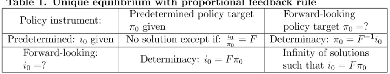
Proposition 1 A unique solution for a single policy instrument responding to a single policy target with a proportional feedback rule i0 = F 0 and a given policy rule parameter
F 6= 0 is obtained when exactly one of the two variables (policy instrument or policy target) is predetermined.
Proof. Let us assume a proportional feedback rule i0 = F 0 with F 6= 0 given. If the
policy target 0 is given (predetermined) and if the policy instrument i0 is not
predeter-mined, then i0 = F 0 is the unique solution for the policy instrument. If the policy target 0 is not predetermined and if the policy instrument i0 is predetermined, then 0 = F 1i0
is the unique solution for the policy target, because F 6= 0. If the policy target 0 and the
policy instrument i0 are predetermined, there is no solution except if F = i0= 0. This line
i0 = F 0 has a zero probability to occur in the continuous plane of the policy instrument
and the policy target that can be chosen: ( 0; i0) 2 R2. If the policy target 0 and the
policy instrument i0 are not predetermined, there is an in…nity of solution according to
the line de…ned by the proportional policy rule i0 = F 0, which is a subspace of
dimen-sion 1 in the plane of the policy instrument and the policy target: ( 0; i0)2 R2. Table 1
summarizes these results.
Table 1. Unique equilibrium with proportional feedback rule Policy instrument: Predetermined policy target
0 given
Forward-looking policy target 0 =?
Predetermined: i0 given No solution except if: i00 = F Determinacy: 0 = F 1i0
Forward-looking:
i0 =? Determinacy: i0
= F 0
In…nity of solutions such that i0 = F 0
The policy transmission mechanism is a …rst order single input (instrument) single output (target) (SISO) model:
t+1= A t+ Bit with B 6= 0 and A 0 (2)
The future value of the policy target is controllable by the current policy instrument because the marginal correlation between the policy instrument and the expectation of the policy target is di¤erent from zero: B 6= 0. The closed-loop system is obtained after substitution of the proportional feedback rule:
t+1 = (A + BF ) t and it= F t= (A + BF ) it 1 (3)
De…nition 1 Determinacy is de…ned by the existence of a bounded and unique (equilib-rium) dynamic path.
Proposition 2 Determinacy of the …rst order single input single output model is obtained in case (1): if exactly one of the two variables (policy target or policy instrument) is predetermined for a set D (1) of policy rule parameters which stabilizes the closed loop system and in case (2) if both variables (policy target and policy instrument) are not predetermined for a set D (0) of policy rule parameters which destabilizes the closed loop system.
Proof. In case (1) exactly one of the two variables (policy target or policy instrument) is predetermined, so that one …nds the unique initial condition for the other variable using the proportional feedback rule (proposition 1). An additional boundary and stability condition implies that the policy rule parameter F belongs to a stability and determinacy set D(1), where one stands for the number of predetermined variables:
F 2 D (1) = fF 2 R such that jA + BF j < 1 with B 6= 0g (4) In case (2), if both the policy target and the policy instrument are forward-looking and if F satis…es the stability condition (F 2 D (1)), there is an in…nity of initial conditions and of stable paths solution. But, if F does not satisfy the stability condition (F =2 D (1)), there is a unique bounded solution where both forward-looking variables jump to their long-run equilibrium: i0 = 0 = 0, which is locally unstable. The instability and determinacy set
D (0) of the policy rule parameter F where zero stands for zero predetermined variable has no intersection with the stability and determinacy set D (1):
F 2 D (0) = fF 2 R such that jA + BF j 1 with B 6= 0g (5)
3
Multiple policy targets
The most common solution of new-Keynesian DSGE models with unique equilibrium satis…es conditions 1 and 2 for the private sector model (Smets and Wouters (2007), Gali (2015)).
Condition 1. The private sector model is based on optimal control, where n state variables are predetermined variables and n co-state variables are forward-looking vari-ables denoted t.
Condition 2. In order to avoid multiple equilibria such as the …scal theory of the price level (Leeper (1991)), the n dynamic equations of controllable predetermined variables of the private sector are removed and substituted by n auto-regressive equations of non-controllable forcing variables zt, equal to the number n of the Euler equations of n
forward-looking variables. For example, one assume zero net supply of predetermined public debt at all dates (Gali (2015), footnote 3).
This private sector model is an hybrid of optimal choice and of ad hoc models. Its transition matrices (A; B; C) do not correspond any longer to a private sector Hamil-tonian matrix because the state variable dynamic equations have been removed:
t+1= A t+ Bit+ Czt (6)
where A, B and C are real matrices of dimension n n and it is a vector of policy
maker’s instruments of dimension n 1, possibly including lags of policy instruments. Let =f 1; :::; ng be an arbitrary set of n complex numbers i such that any i with
Im( i)6= 0 appears in in a conjugate pair.
Theorem 3 Wonham (1967) pole placement. The pair (A; B) is controllable, sat-isfying the condition rank (B; AB; A2B;:::; An 1B) = n, if and only if, for every choice
of the set =f 1; :::; ng, there is a matrix F such that A + BF has for its sets of
eigenvalues.
Wonham’s (1967) pole placement theorem states that linear feedback rule parameters are bifurcation parameters of controllable linear systems. Close to bifurcations limit values, a small change of the policy rule parameters leads to big qualitative change of the dynamics of the system to be controlled, as eigenvalues shifts from being outside the unit circle to inside the unit circle.
A proportional feedback rule it = F t + Fzzt, where F and Fz are real matrices
of dimension n n (F is assumed to be invertible and Fz may be equal to the null
matrix), is substituted in the policy transmission mechanism in order to …nd the closed loop model, with the controllable feedback matrix A + BF :
t+1 = (A + BF ) t+ (C + BFz) zt (7)
Proposition 4 When all controllable policy targets are n forward-looking variables with a transmission mechanism de…ned by the controllable pair (A; B) with A and B be real matrices of dimension n n and when all non-controllable variables are n stationary auto-regressive and predetermined shocks, determinacy is obtained in case (1): all the n policy instruments (including if necessary lags of policy instruments) are predetermined, for a set D (n) of policy rule parameters corresponding to a real and invertible matrix F of dimension n n which stabilizes the closed loop system A + BF with n controllable eigenvalues i(A + BF ) inside the unit circle and in case (2): all the n policy
instru-ments are not predetermined for a set D (0) of policy rule parameters F which destabilizes the closed loop system A + BF with all n controllable eigenvalues i(A + BF ) outside
the unit circle.
Proof. In case (1), exactly half of the variables (policy target or policy instrument) are predetermined, so that there is a unique initial condition for the other variable if F is invertible: 0 = F 1i0 F 1Fzz0. If the matrix F is not invertible, this means
combination of other policy rules. Using Wonham (1967) theorem, an additional boundary and stability condition implies that the policy rule parameters F belongs to a stability and determinacy set D(n), where n stands for the number of endogenous predetermined variables equal to the number of policy instruments:
F 2 D (n) = fF 2 Rn Rn such that: i(A + BF) < 1 for 1 i n g (8)
In case (2), if both the policy targets and the policy instruments are forward-looking and if F satis…es the stability condition (F 2 D (m)), there is an in…nity of initial conditions and of stable paths solution. But, if F belongs to a set destabilizing all the m eigenvalues of the controllable system, there is a unique bounded solution such as it = F t =
F N zzt, when N z is a unique projection matrix, which is a locally unstable equilibrium
path. Both forward-looking policy targets and policy instruments are linear functions of auto-regressive shocks. Using Wonham (1967) theorem, the instability and determinacy set D (0) of the policy rule parameters F where zero stands for zero endogenous and predetermined variable is de…ned by:
F 2 D (0) = fF 2 Rn Rn such that: i(A + BF) 1 for 1 i n g (9)
Example 1 DSGE models with (possibly optimal) simple proportional …scal, macro-prudential and Taylor rules and discretionary optimal policy are solved according to the determinacy theory assuming that policy instruments are forward-looking when policy tar-gets are forward-looking.
Example 2 The solution of the Ramsey optimal policy under quasi-commitment with a non-zero probability to renege commitment (Roberds (1987)) for the same DSGE model of the private sector corresponds to the determinacy theory which assumes that policy in-struments are backward-looking when policy targets are forward-looking. Ramsey optimal policy under quasi-commitment sets optimal initial condition for policy instruments such that the marginal value of the loss function with respect to each forward-looking policy tar-get (the Lagrange multiplier associated to each forward-looking policy tartar-get) is equal to zero, at each re-optimization. Hence, it is a DEDUCTED result (not a CHOSEN assump-tion) that policy instruments are predetermined when policy targets are forward-looking. For Ramsey optimal policy under quasi-commitment, the initial conditions provide an optimal initial anchor with a relation it = N t = Nzzt, with optimal projection
ma-trices N and Nz, which is the same of the next period only if the policy maker renege
commitment with a probability 1 q. Else the policy instruments behave according to the optimal policy rule it= F t+ Fzzt with a probability of not reneging commitment equal
to q for q 2 ]0; 1]. Discretionary optimal policy corresponds to the case of a policy maker who continuously renege commitment: q = 0 at any instant and for ever in an in…nite horizon (Chatelain and Ralf (2018a)).
Example 3 DSGE models with (possibly optimal) simple proportional …scal, macro-prudential and Taylor rules and discretionary optimal policy are solved according to the determinacy theory assuming that policy instruments are backward-looking with given initial conditions when policy targets are forward-looking, although this is not the usual convention.
Table 2 summarizes the results and the appendix provides more details. Table 2. Multiple policy targets
Authors Vaughan (1970) Roberds (1987) Blanchard Kahn
Model Linear quadratic regulator Ramsey optimal policy Ad hoc
Agents Private sector model Leader: Policy maker Policy rule
Variables
n predetermined states: private sector targets and policy maker targets
CHOSEN
THEN SET TO ZERO
0forward-looking co-state variable DEDUCTED 0 predetermined CHOSEN Variables n forward-looking costates private sector instruments and policy maker targets
DEDUCTED n predetermined costates policymaker instruments DEDUCTED n forward-looking -CHOSEN Matrix An+ BnF Euler equations H2n: H
0
2n= J2nH2n1J 1
2n An+ BnF
Eigenvalues - n stable j ij < 1 n depends on F
Eigenvalues - n unstable 1
j ij > 1 m depends on F
Determinacy - Always F so that: n = 0
Parameters - F 2 D (n) F 2 D (0)
Exogenous k = npredetermined zt n predetermined zt n predetermined zt
Eigenvalues k = n stable j ij < 1 n stable j ij < 1 n stable j ij < 1
Policy rule - it = F t+ Fzzt it = F t = Nzzt
Credibility - q 2 ]0; 1] q = 0
4
Criteria for Forward-looking versus Predetermined
Policy Instruments
For the internal validity of the determinacy theory of feedback rules, Blanchard and Kahn (1980) contribution does not prove nor disprove that policy instruments responding to forward-looking variables with ad hoc proportional rules should be forward-looking or predetermined (see appendix).
For its external validity, Beyer and Farmer (2003, 2009) proved that any indeterminate model could be observationally equivalent to a determinate model, although one model has more parameters than the other.
Both from the point of internal validity (this paper) and from the point of view of external validity (Beyer and Farmer (2003)), the determinacy theory of feedback rules cannot be proven wrong nor right. Like Socrates in Plato’s early dialogues, we have reached aporia ( o ), an improved state of indeterminacy, still not knowing what to say about determinacy versus indeterminacy. To go beyond this aporia, we propose the following set of criteria.
Criterion 1 Microeconomic foundations: reject ad hoc equations and ad hoc de…nition of which variables are forward-looking.
Criterion 2 Robustness to misspeci…cation. A policy maker using negative-feedback pol-icy rule parameters when he does not know exactly the model may have more robust polpol-icy
results with respect to stabilization (Hansen and Sargent (2008), Giordani and Söderlind (2006), Chatelain and Ralf (2018a)).
Criterion 3 Practical impossibility of perpetual continuous re-optimization reneging com-mitment at every instant in the in…nite horizon ("discretion" micro-foundation). Discrete-time discontinuous optimization corresponds to Ramsey optimal policy under quasi com-mitment, as there is a time interval between dates where policy remains unchanged. The probability of the event of a probability exactly equal to zero of not reneging commitment fq = 0g against all the events fq 2 ]0; 1]g, including extremely small but distinct from zero probability of not reneging commitment corresponds to a Dirac distribution, with a zero prior probability on the event fq = 0g (Chatelain and Ralf (2018a)).
Three other criteria are based on Ockham’s razor (Chatelain and Ralf (2018b)), . Criterion 4 Ockham’s razor (1) on the number of parameters: For two observationally equivalent models where model (2) includes more parameters than model (1), prefer model (1).
Criterion 5 Ockham’s razor (2) on lack of identi…cation and weak identi…cation: For two observationally equivalent models when model (2) includes more parameters facing exact identi…cation or weaker identi…cation issues than in model (1), prefer model (1). Criterion 6 Ockham’s razor (3) on complicated explanations: For two observationally equivalent models, when model (2) proposed a more complicated mechanism than model (1), prefer model (1). For example, when policy instruments and policy targets are both forward-looking, the policy rule parameters e¤ect goes through the denominator of the slope of eigenvectors of stable eigenvalues. When policy instruments are predetermined and policy targets forward-looking, the policy rule parameters increase or decrease the numerator of growth or convergence factors of policy targets (the eigenvalues): it is the usual feedback e¤ect of control theory.
5
Conclusion
Blanchard and Kahn (1980) paper does not prove that policy instrument are forward-looking instead of predetermined variables when the policy targets are forward-forward-looking. Hence, there is an indeterminacy of the determinacy theory with ad hoc proportional feedback rules. For a similar convention, clocks may have hands that move clockwise versus counter-clockwise around their twenty-four-hours dial (like Paolo Uccelo’s clock in Florence cathedral) versus around their twelve-hours dial (Arthur (1990)).
Six criteria favor the assumption that policy instruments should be predetermined when the policy targets are forward-looking. This suggests that DSGE models are currently locked in to the inferior technology path of having chosen the convention of forward-looking policy instrument if policy targets are forward-looking, as it happened for QWERTY typewriter keyboard (David (1985)).
References
[1] Anderson E.W., Hansen L.P., McGrattan E.R. and Sargent T.J. (1996). Mechanics of Forming and Estimating Dynamic Linear Economies. in Amman H.M., Kendrick D.A. and Rust J. (editors) Handbook of Computational Economics, Elsevier, Ams-terdam, 171-252.
[2] Arthur, W. B. (1990). Positive feedbacks in the economy. Scienti…c american, 262(2), 92-99.
[3] Blanchard O.J. and Kahn C. (1980). The solution of linear di¤erence models under rational expectations. Econometrica, 48, 1305-1311.
[4] Beyer, A., & Farmer, R. E. (2003). On the indeterminacy of determinacy and inde-terminacy. ECB working paper 277.
[5] Beyer, A., & Farmer, R. E. (2007). Testing for indeterminacy: An application to US monetary policy: Comment. American Economic Review, 97(1), 524-529.
[6] Chatelain J.B. and Ralf K. (2014). Stability and Identi…cation with Optimal Macro-prudential Policy Rules. MPRA working paper.
[7] Chatelain, J. B., and Ralf, K. (2014). Peut-on identi…er les politiques économiques stabilisant une économie instable? Revue française d’économie, 29, pp. 143-178. [8] Chatelain J.B. and Ralf K. (2014). A Finite Set of Equilibria for the Indeterminacy
of Linear Rational Expectations Models. MPRA paper.
[9] Chatelain J.B. and Ralf K. (2016). Countercyclical versus Procyclical Taylor Prin-ciples. SSRN working paper.
[10] Chatelain J.B. and Ralf K. (2017a). A Simple Algorithm for Solving Ramsey Optimal Policy with Exogenous Forcing Variables. PSE and SSRN working paper.
[11] Chatelain J.B. and Ralf K. (2017b). Can we Identify the Fed’s Preferences? PSE and SSRN working paper.
[12] Chatelain, J. B., & Ralf, K. (2018a). Imperfect Credibility versus No Credibility of Optimal Monetary Policy. PSE and SSRN working paper.
[13] Chatelain, J. B., & Ralf, K. (2018b). Publish and Perish: Creative Destruction and Macroeconomic Theory. History of Economic Ideas, 3, forthcoming.
[14] Chatelain, J. B., & Ralf, K. (2018c). Super-inertial policy rules are not solution of Ramsey optimal monetary policy. PSE and SSRN working paper.
[15] Cochrane J.H. (2011). Determinacy and identi…cation with Taylor Rules. Journal of Political Economy, 119, 565-615.
[16] David, P. A. (1985). Clio and the Economics of QWERTY. The American economic review, 75(2), 332-337.
[17] Debortoli, D., and Nunes, R. (2014). Monetary regime switches and central bank preferences. Journal of Money, Credit and Banking, 46, pp. 1591-1626.
[18] Gali J. (2015). Monetary Policy, In‡ation and the Business Cycle. 2nd edition, Princeton University Press, Princeton.
[19] Giordani and Söderlind [2004]. Solution of Macromodels with Hansen-Sargent Ro-bust Policies: some extensions. Journal of Economic Dynamics and Control, 12, 2367-2397.
[20] Hansen L.P. and Sargent T. (2008). Robustness, Princeton University Press, Prince-ton.
[21] Hansen L.P. and Sargent T. (2011). Wanting Robustness in Macroeconomics. In Handbook of Monetary Economics, vol 3(B), Friedman B.M. and Woodford M. edi-tors, Elsevier B.V., pp. 1097-1155.
[22] Kalman R.E. (1960). Contributions to the Theory of Optimal Control. Boletin de la Sociedad Matematica Mexicana, 5, pp. 102-109.
[23] Leeper, E. M. (1991). Equilibria under ‘active’and ‘passive’monetary and …scal poli-cies. Journal of monetary Economics, 27, pp. 129-147.
[24] Ljungqvist L. and Sargent T.J. (2012). Recursive Macroeconomic Theory. 3rd edition. The MIT Press. Cambridge, Massaschussets.
[25] Roberds, W. (1987). Models of policy under stochastic replanning. International Economic Review, 28, pp. 731-755.
[26] Schaumburg, E., and Tambalotti, A. (2007). An investigation of the gains from commitment in monetary policy. Journal of Monetary Economics, 54, pp. 302-324. [27] Simaan, M., & Cruz, J. B. (1973). Additional aspects of the Stackelberg strategy
in nonzero-sum games. Journal of Optimization Theory and Applications, 11, pp. 613-626.
[28] Smets, F., and Wouters, R. (2007). Shocks and frictions in US business cycles: A Bayesian DSGE approach. The American Economic Review, 97, 586-606.
[29] Vaughan, D. (1970). A nonrecursive algebraic solution for the discrete Riccati equa-tion. IEEE Transactions on Automatic Control, 15, 597-599.
[30] Wonham W.N. (1967). On pole assignment in multi-input controllable linear system. IEEE transactions on automatic control. 12, pp. 660-665.
6
Appendix: Optimal Control versus Blanchard and
Kahn (1980)
This appendix recalls background informations on Blanchard and Kahn (1980) and on the linear quadratic regulator.
Blanchard and Kahn’s (1980), p.1305, states that the matrices A and of their dynamic model are ad hoc given matrices which are not derived from intertemporal optimal choice. The transition matrix A has a given number n of stable eigenvalues inside the unit circle and a remaining number m of unstable eigenvalues outside the unit
circle. They also state that the choice of which variables are predetermined or forward-looking and their numbers n and m are given. In practice, these numbers n, m, n, m are discretionary ad hoc choices done by the researcher:
The model is given as follows: Xt+1
tPt+1
= A Xt
Pt
+ Zt; Xt=0 = X0 (10)
where X is an (n 1)vector of variables predetermined at t; P is an (m 1) vector of variables non-predetermined at t; Z is an (k 1)vector of exogenous variables;tPt+1is the agents expectations of Pt+1held at t; A, are (n + m)
(n + m) and a (n + m) k matrices, respectively.
tPt+1 = Et(Pt+1 p t) : (11)
where Et( ) is the mathematical expectation operator; t is the information
set at date t,.... A predetermined variable is a function only of variables known at date t, that is of variables in t that Xt+1 = tXt+1 whatever the
realization of the variables in t+1. A non-predetermined variable can be
a function of any variable in t+1, so that we can conclude that Pt+1=tPt+1
only if the realization of all variables in t+1 are equal to their expectations
conditional on t.
Their model is an ad hoc linear rational expectations model of the 1970s. Their example 4 is an ad hoc multiplier accelerator model including only one non-predetermined (or forward-looking or jump) variable: output. They show that a researcher can choose which variable is a predetermined or a non-predetermined variable independently from an economic criterion such as real versus nominal variables (p.1307):
This example also shows the absence of necessary connection between "real," "nominal" and "predetermined," "non-predetermined".
Set aside this sentence, Blanchard and Kahn (1980) paper do not provide any criterion for deciding when a variable is forward-looking or not. In their example of the multiplier accelerator model, the demand components of output: consumption, investment and government expenditures may all have been assumed to depend on forward-looking spe-ci…c expectations of consumption, investment and government expenditures, instead of depending only on aggregate output expectations.
Blanchard and Kahn (1980), p.1307, set a stability boundary condition in the in…nite horizon, like the in…nite horizon transversality conditions assumed in optimal control:
This condition in e¤ect rules out exponential growth of the expectations of Xt+1 and Pt+1 held at time t. (This in particular rules out "bubbles"...).
Vaughan (1970) proposed a solution of the Hamiltonian system of the linear quadratic regulator using the Jordan canonical form of the Hamiltonian matrix H. The Hamiltonian includes Lagrange multipliers which are jump variables. Their number m is necessarily equal to the number n of predetermined variables. Because the Hamiltonian matrix H is similar to its inverse (symplectic matrix), the number n of stable eigenvalues of the
matrix H inside the unit circle is equal to the number of unstable eigenvalues m outside the unit circle. We then have n = n = m = m.
Blanchard and Kahn (1980), p.1307, proceed by analogy using Vaughan (1970) solu-tion using Jordan canonical form. Their ad hoc given matrix A can have an ad hoc given number of stable eigenvalues n which can be di¤erent from the ad hoc given number of predetermined variables n:
Our strategy is to simplify the model by transforming it into its canonical from, following Vaughan (1970). Thus A is …rst transformed into Jordan canonical form: A = C 1JCwhere the diagonal elements of J, which are the eigenvalues of A, are ordered by increasing absolute value.
Vaughan (1970) seeks the unique optimal policy rule that restricts 2n variables of the Hamiltonian system remain in the stable subspace of dimension n of the Hamiltonian matrix of dimension 2n. This optimal policy rule is such that n forward-looking variables are a unique linear function of n predetermined variables.
It should be clearly understood that the "real world" dimensions, corresponding to the number of (state) variables that should be stabilized in the LQR optimal control is equal to n. Doubling the dimensions to 2n in the Hamiltonian system is an artefact of the intermediate computations proposed by Lagrange. The fact that an Hamilonian system has a saddle-point equilibrium property in dimension 2n does not imply that the system of dimension n to be controlled is locally instable. The in…nite horizon transversality conditions are assumed on purpose to stabilize the system of n state variables in optimal control.
Blanchard and Kahn (1980), p.1308, determinacy proposition is:
Proposition 1: If m = m, i.e., if the number of eigenvalues of A outside the unit circle is equal to the number of non-predetermined variables, then there exists a unique solution.
This proposition is satis…ed for the linear quadratic regulator, because Blanchard and Kahn (1980) solution is an extension of Vaughan (1970) solution of the LQR to ad hoc models including jump variables. Blanchard and Kahn (1980), p.1309, acknowledge that all optimal intertemporal choice models have the determinacy property:
How likely are we to have m = m in a particular model? It may be that the system described by (10) is just the set of necessary conditions for maximization of a quadratic function subject to linear constraints. In this case, the matrix A will have more structure than we have imposed here, and the condition m = m will always hold.
The linear quadratic model is also a local approximation around an equilibrium of non-quadratic non-linear optimal control problems such as optimal saving and optimal growth models under adequate concavity assumptions. As acknowledged by Blanchard and Kahn (1980), p.1309, these optimal saving and optimal growth models can be solved by the Lagrange method (but not necessarily) with Hamiltonian systems having the same saddle-point property as the linear quadratic regulator:
The condition m = m is also clearly related to the strict saddle point property discussed in the context of growth models: the above proposition (1) states in e¤ect that a unique solution will exist if and only if A has the strict saddlepoint property.
Blanchard and Kahn (1980) determinacy condition is only a contribution for ad hoc linear models including forward-looking variables. Optimal intertemporal choice models always satisfy the determinacy condition under adequate concavity conditions: this has been proven in papers of optimal control before Blanchard and Kahn (1980), such as Vaughan (1970) and Kalman (1960).
The wording "rational expectations" in Blanchard and Kahn (1980) is misleading. Because they abandoned rationality, their linear algebra contribution cannot explain why and how agents choose expectations of the unique bounded solution instead of unstable paths created by policy maker’s policy rule in the determinacy theory (Cochrane (2011)). Insights on rational expectations are obtained with Kalman …lter estimations solv-ing Muth’s problem (Hansen and Sargent (2008)) and Ramsey optimal policy based on linear quadratic rational behaviour (Ljungqvist and Sargent (2012), Hansen and Sargent (2008)). In these models, Blanchard and Kahn (1980) determinacy condition is always achieved.
We compare step by step the general solutions of optimal control, of Ramsey optimal policy under quasi-commitment and of Blanchard and Kahn (1980) ad hoc model.
1. All models begins with an identical dynamic linear model for predetermined state variables which is CHOSEN by the researcher. Predetermined variable can be split in two sets. A …rst set includes a set of variables which are controllable by the economic agents. A second set includes non-controllable exogenous variables which are usually auto-regressive shocks, with stable eigenvalues (auto-regressive parameters below one in absolute values).
2. The …rst key distinction is that forward-looking variables are CHOSEN to be so by the researcher in Blanchard Kahn (1980) whereas jump variables are DEDUCTED to be so from the mathematical method of optimal control approximated by a linear quadratic regulator and Stackelberg dynamic game.
3. The second key distinction are the equations related to jump variables. They corre-sponds to …rst order conditions (Euler equations) which are endogenously DEDUCTED in the optimization problem in optimal control and Stackelberg dynamic game. They are arbitrarily CHOSEN, such as, for example, proportional …scal, macro-prudential or Taylor rule in Blanchard and Kahn (1980).
4. When the determinacy condition is satis…ed, then the solution proceeds for all models with the same algorithms solving a Riccati equation or, equivalently, using the method of undetermined coe¢ cients in order to anchor forward-looking variables to be exactly collinear with predetermined variables according to an "optimal control policy rule" (control models) or to a "determinacy policy rule" (Blanchard and Kahn (1980) model). However the dimension of the stable subspace may not be the same, because the number of predetermined variables can be di¤erent in Blanchard and Kahn (1980) with respect to optimal control models.
These results are summarized in table 3. Table 3. General case comparison
Authors Vaughan (1970) Roberds (1987) Blanchard Kahn
Model Linear quadratic regulator Ramsey optimal policy Ad hoc
Agents Private sector model Leader: Policy maker Policy rule
Variables
n predetermined states: private sector targets and policy maker targets
CHOSEN n forward-looking costate variables policymaker instruments DEDUCTED n predetermined -CHOSEN Variables n forward-looking costates private sector instruments and policy maker targets
DEDUCTED n predetermined costate variables policymaker instruments DEDUCTED m forward-looking -CHOSEN Matrix H2n: H 0 2n = J2nH2n1J 1 2n H4n: H 0 4n= J4nH4n1J 1 4n Any matrix: An+m
Eigenvalues n stable j ij < 1 2n stable j ij < 1 n stable
Eigenvalues n unstable j1
ij > 1 2n unstable
1
j ij > 1 m unstable
Determinacy Always Always IF n = n, m = m
Exogenous k predetermined zt k predetermined zt k predetermined zt
Eigenvalues k stable j ij < 1 k stable j ij < 1 k stable j ij < 1