Computational Microscopy for Sample Analysis
by
Hayato Ikoma
B.E., the University of Tokyo (2010)
M.S., Kyoto University (2012)
Submitted to the the Program in Media Arts and Sciences,
School of Architecture and Planning
in partial fulfillment of the requirements for the degree of
Master of Science in Media Arts and Sciences HN
at the
JUL
14
2014
MASSACHUSETTS INSTITUTE OF TECHNOLOGY
LIBRARIES
June 2014
© Massachusetts Institute of Technology 2014. All rights reserved.
Signature redacted
A uthor...
Pro am in Media Arts and Sciences
May 9, 2014
Certified by
...
Signature redacted...
Ramesh Raskar
Associate Professor
Thesis Supervisor
Signature redacted
Accepted by ...
...
a Maes
Associate Academic Head,
Program in Media Arts and Sciences
Computational Microscopy for Sample Analysis
by
Hayato Ikoma
Submitted to the the Program in Media Arts and Sciences, School of Architecture and Planning
on May 9, 2014, in partial fulfillment of the requirements for the degree of
Master of Science in Media Arts and Sciences
Abstract
Computational microscopy is an emerging tcchnology which extends the capabilities of optical microscopy with the help of computation. One of the notable example is super-resolution fluorescence microscopy which achieves sub-wavelength super-resolution. This thesis explores the novel application of computational imaging methods to fluores-cence microscopy and oblique illumination microscopy. In fluoresfluores-cence spectroscopy, we have developed a novel nonlinear matrix unmixing algorithm to separate fluores-cence spectra distorted by absorption effect. By extending the method to tensor form, we have also demonstrated the performance of a nonlinear fluorescence tensor unmix-ing algorithm on spectral fluorescence imagunmix-ing. In the future, this algorithm may be applied to fluorescence unmixing in deep tissue imaging. The performance of the two algorithms were examined on simulation and experiments. In another project, we applied switchable multiple oblique illuminations to reflected-light microscopy. While the proposed system is easily implemented compared to existing methods, we demonstrate that the microscope detects the direction of surface roughness whose height is as small as illumination wavelength.
Thesis Supervisor: Ramesh Raskar Title: Associate Professor
Computational Microscopy for Sample Analysis
by
Hayato Ikoma
Signature
redacted
T hesis A dvisor ... . .. ... Ramesh Raskar Associate Professor Program in Media Arts and SciencesSignature redacted
Thesis Reader... ...
V. Michael Bove, Jr. Principal Research Scientist MIT Media Lab
Signature redacted'
Thesis Reader...Edward Boyden Associate Professor Program in Media Arts and Sciences
Acknowledgments
In this thesis, I integrated my knowledge of materials, biology and applied mathe-matics, which I have studied through my research career. I would like to express my gratitude to all of the people I have met since my undergraduate research.
I thank my advisor, Ramesh Raskar, for selecting me as a graduate student. I am
grateful for all of his supports.
Thank you to Mike Bove and Ed Boyden, for being my thesis reader. I appreci-ate their help.
Thanks to the Camera Culture group members. I am very grateful to Barmak Hesh-mat and Gordon Wetzstein, who guided me to conduct research at Camera Culture group. Without their help, I would not have accomplished my research here.
Thank you to Keisuke Ishihara, my friend at Harvard Medical School, who helped me biological samples until late night for several days in a row.
Thank you to all of my Media Lab friends, especially Deepak Jagdish and Dan Sawada.
My life at the Lab was enjoyable because of their friendship and supports.
Thanks to Natura. Their fluorescence spectroscopy datasets of hair inspired me to come up with new research ideas.
Thanks to Olympus, who provided us high-quality lenses and let us use them for any research projects. I appreciate their flexibility.
A Special thank you to Funai Overseas Scholarship, which fully supported my
Contents
1 Introduction
2 Nonlinear Fluorescence Unmixing for Spectroscopy and Microscopy 13
2.1 Proposed Method and Related Work . . . . 2.2 T heory . . . . 2.2.1 Model of Fluorescence Spectrophotometer Measurements 2.2.2 Nonlinear Fluorescence Matrix Unmixing . . . .
2.2.3 Model of Fluorescence Spectra from Tissue in Depth . . 2.2.4 Nonlinear Fluorescence Tensor Unmixing . . . .
2.3 Sim ulation . . . .
2.3.1 Generation of Spectroscopic Data . . . .
2.3.2 Performance Analysis . . . .
2.3.3 Generation of Spectral Imaging Datasets . . . . 2.3.4 Performance Analysis . . . . 2.4 Experimental Results . . . . 2.4.1 Fluorom eter . . . . 2.4.2 Fluorescence Microscopy . . . .
2.5 D iscussion . . . .
2.5.1 Benefits and Limitations . . . .
2.5.2 Future W ork . . . .
3 Switchable Multiple Oblique Illumination Microscopy
3.1 Proposed Method and Related Work . . . .
11 13 15 15 17 18 19 20 21 21 23 24 26 26 26 28 28 29 31 31
3.2 Method . . . .. . . . . 32
3.2.1 Hardware Implementation . . . . 32
3.2.2 Sample Preparation . . . . 33
3.3 Result . . . . 33
3.4 Discussion . . . . 35
3.4.1 Benefits and Limitations . . . . 35
3.4.2 Future Direction . . . . 38
Chapter 1
Introduction
Optical microscopy is a fundamental research tool in engineering and science. Through its 400-year history, numerous optical systems have been proposed to visualize mi-crostructures that cannot be seen with naked eyes
[1].
Since the introduction of digital image acquisition and image processing, computers have been more and more integrated with optical microscopy [2].As is happening in computational photography and display [3, 4, 5, 6, 7], the com-bination of optical microscopy and signal processing is creating new capabilities. This emerging field is called computational microscopy. Most computational microscopy techniques acquire several images under different illumination condition and computes a synthesized image. By combining active illumination and signal processing, optical microscopy can reveal structures which is invisible only with an optical imaging sys-tem. For example, LC-PolScope and orientation-independent differential interference microscope (OI-DIC) acquire images under differently-polarized light illumination and quantitatively compute birefringence and refractive index, respectively [8, 9]. Struc-tured illumination microscopy (SIM) illuminates a sample with differently-rotated grid patterns and generate a superresolution image [10]. Single-molecule localization microscopy, such as STORM and PALM, also reconstructs a superresolution image from images each of in which a subgroup of fluorescent molecules are stochastically excited [11, 12].
illumination for the application to computational optical microscopy. Chapter 2 de-scribes the theory and performance of nonlinear fluorescence unmixing for fluorescence spectroscopy and microscopy. Chapter 3 reports the development of the switchable multiple oblique illumination microscopy and its application.
Chapter 2
Nonlinear Fluorescence Unmixing
for Spectroscopy and Microscopy
2.1
Proposed Method and Related Work
Fluorescence spectroscopy is a widely-used technique in many fields, such as analyti-cal chemistry, environmental sciences and medicine. Since fluorescence spectra reflect the state and type of molecules, the analysis of fluorescence spectra nondestructively provides molecular information of a sample. For example, the analysis of autofluo-rescence, which is naturally emitted by a sample, has been used for the detection of cancer, contamination in water and degradation of food [13]. In addition, fluorescence spectral imaging system, where each pixel has spectral information, has expanded the capability of microscopy.
In the analysis of fluorescence spectra, the separation of fluorescence is of great importance. Most analyzed samples for fluorescence spectroscopy, including blood, water and food, have multiple fluorophores. Furthermore, it is common for fluores-cence microscopy to label biological samples with multiple fluorophores. The mea-sured fluorescence spectrum from those samples is a sum of the spectrum of each fluorophore. If their individual spectra do not significantly overlap, the fluorescence light can be separated by optical filters. However, severely-overlapping spectra can-not be separated optically. In those cases, a mathematical technique, called linear
unmixing (LU), is often used to separate them.
LU is an algorithm which decomposes the total fluorescence into each fluorophore's
contribution [14]. This algorithm works on the assumption that a sample's absorbance is negligible. On this assumption, the measured signal can be considered to be a linear combination of each fluorescence spectrum. Therefore, by using premeasured emission spectrum for each fluorophore, these linear equations can be solved when the number of channels recorded is larger than the number of fluorescence species. This method has been successfully applied to fluorescence spectroscopy and multi-channel fluorescence light microscopy [15, 16].
In addition to LU, under the assumption of negligible absorption, blind unmixing methods have been developed with mathematical tools, such as nonnegative matrix factorization (NMF) and parallel factor analysis (PARAFAC), also known as
CAN-DECOMP and CP decomposition [17]. In many cases, to conduct blind unmixing,
excitation and emission matrix (EEM) of a sample is measured. EEM is composed of a series of emission spectra measured with different excitation wavelengths. In a single fluorophore case, its EEM can be described as an outer product of its excitation spectrum and emission spectrum, while its intensity is proportional to its concentra-tion. Therefore, the EEM of a sample containing several fluorophores has trilinearity.
NMF and PARAFAC exploit this multilinearity of fluorescence.
However, when the sample's absorption is not negligible, the measured fluorescence spectra are distorted by the wavelength-dependent absorption, which is called inner filter effect. This nonlinear effect disables the introduced linear unmixing algorithms. This inner filter effect has been a major problem for fluorescence spectroscopy, and numerous techniques have been proposed to recover the intrinsic fluorescence spectra from the distorted measurements [18]. All of the methods have their own advantages and disadvantages. For example, liquid samples can be diluted to the extent where absorption is negligible [19, 20]. Even though this procedure can provide accurate estimation of intrinsic fluorescence spectra, it cannot be applied to solid materials. On the other hand, Monte Carlo simulations for the inner filter effect correction with photon migration theory can be performed on solid materials [21, 22]. However, they
require expensive computation.
In this thesis, we propose a novel nonlinear unmixing method to estimate abun-dance of fluorophores in a light-absorbing sample for fluorescence spectroscopy and microscopy. In particular, we make the following contributions:
" We introduce a model of fluorescence spectra from a light-absorbing sample as a matrix representation. We also model spectral fluorescence imaging of a light-absorbing sample as a tensor representation.
. Based on the matrix and tensor representations, we introduce a new nonlinear unmixing method to estimate abundances of fluorophores by using nonnegative matrix and tensor factorization. This method does not require any additional measurements and can be applied to both liquid and solid samples.
. We evaluate the performance of the unmixing method on simulated fluorescence spectra and spectral images.
. We show that the nonlinear unmixing method experimentaly outperforms the conventional linear unmixing method.
2.2
Theory
In this section, we model the spectra of mixture of fluorophores in a light-absorbing medium and propose the algorithms to estimate each fluorophore's contributions from the model. We consider a conventional fluorometer and a fluorescence microscope as a measurement system.
2.2.1
Model of Fluorescence Spectrophotometer Measurements
There have been many attempts to model fluorescence spectra affected by absorption effect in fluorometer measurements [18]. Based on the Beer-Lambert law, Luciani et al. mathematically described the absorption effect in a fluorescence spectroscopy
albf a2b
M = (C1 + C2 n+ .+CN M )
Measured Attenuation Fluorophore I Fluorophore 2 FluorophoreN
EEM EEM EEM EEM
TW [ ai, bi, ciI [a2, b2, c2] [aN,bN, CN
Figure 2-1: Noiseless EEM model affected by absorption effect. The top row is the visualization of Equation 2.2. The bottom row is the visualization of Equation 2.11.
measurement in detail [19]. Following their formulation, the measured fluorescence intensity F(Aex, Aem) can be described as:
N
F(Aex, Aem) = M11l-(A(Aex)+A(Xem))/2
S
Io(Aex)#nCn-n(Aex)^/n(Aem) + e, (2.1)n=1
where e is the measurement noise, Aex and Aem are the excitation and emission wave-length, IO(A) is the intensity of the illumination, A(A) is the absorption spectrum of the solution, M1 is a wavelength-independent constant factor, N is the number of
flu-orophores in the sample,
#m, cn, En and 7n are the quantum yield, the concentration,
the molar extinction coefficient and the emission spectrum of the fluorophore n.Let N columns of the matrix A = [ai, a2, ... , aN] and B = [bi, b2, ... , bN] be
de-fined as the emission and excitation spectrum of fluorophores, where ant() =
#nEn(Aj)
and bn(j) = Io(Aj)-n(Aj). The equation (2.1) can be rewritten in discretized matrix representation as:F = M1(wiwT) * ADBT + E, (2.2)
where Fjj = F(A2, Aj), wi(i) = 1 0 A(A)/27 W2(j) = 1 0-A(A 3)/2, D = diag(ci, c2, . . . , CN)
and E is a random noise matrix. A * B denotes the Hadamard product (elementwise product) of A and B. Equation 2.2 is illustrated in Figure 2-1.
aNbN
2.2.2
Nonlinear Fluorescence Matrix Unmixing
Here, we describe the way to estimate D from the measurement F in the equation (2.2). This estimation problem can be described as the following minimization prob-lem:
min - ||F - (W1iW) ABT||FD
W1, W2, D
subject to 0 i1, 2 1, O .
I F denotes the Frobenius norm. W, (r = 1, 2) and D = diag(C, 2,. ..,2FN) are
the estimations of wp and D, respectively. Since this minimization problem has scale ambiguities, the estimated values Wr and D are not the absolute concentrations. However, this does not become a problem, because most chemical analysis demands only the ratio of components. As in LU, we assume the emission and excitation spectra of fluorophores can be used separately.
To solve this problem, we derive new update rules by modifying the multiplicative update rules employed for nonnegative matrix factorization [23]:
((B * W2) O (A * W1)) vec(F) C <- * _- ,- (2.4) ((B * W2) ( (A o 1)((B ( W2) (A ( W1))-C ((ADBT) ® F)W2 wi < (2.5) ((ADBT) (ADBT))(W2 @ 2) ((ADBT) ® F)W 1 ( W2 <-(2.6) ((ADBT) * (ADBT))T( 1 W 1
where Wr (r 1, 2) is a N-column matrix whose columns are identical horizontal copies of the column vector ' r and i =
[s1,a
2,...,
T. During the updates of 'cand W'r, D and Wr are updated accordingly. 0 represents the Khatri-Rao product, defined as
P ® Q=[p1®qi p 2 0q 2 ... PK &qK] (2.7)
for matrices P c RIxK and
Q
E RJxK. ® represents the Kronecker product operator,nonlinear fluorescence matrix unmixing (NFMU), which decomposes a nonlinearly-distorted EEM.
2.2.3
Model of Fluorescence Spectra from Tissue in Depth
Recently, mainly in neuroscience, there is a growing need to capture images of neu-ronal activities through significant depths of the brain. To meet this demand, multi-photon microscopy is becoming a basic tool to visualize neurons [24, 25]. Furthermore, in addition to conventional multilabel approach, a stochastic expression of multiple fluorescence proteins is used to label neurons with approximately 100 colors [26, 27]. However, the model of fluorescence spectra from deep tissues has not been investi-gated in detail so far.In fluorescence microscopy, a captured image is the convolution of the point spread function (PSF) of the imaging system and the distribution of fluorophores in a sample. The PSF depends on excitation and emission wavelength. Therefore, if the bandwidth of exploited excitation and emission wavelength are wide, deconvolution should be performed on the captured images beforehand to analyze spectra [28]. Hereafter, we base our discussion on deconvolved images and images where the convolution effect is negligible.
In a p-photon process, the intensity of fluorescence from N types of fluorophores contributing to the signal of pixel k is proportional to the sum of the product of the
excitation spectrum sn(Aex), the emission spectrum tn(Aem), the abundance un of the
fluorophore n:
N
fk(Aex, Aem) = M 2Eo(Ae)PZ Sn(Aex)tn(Aem)Uk,n, (2.8)
n=1
where M 2 is a wavelength-independent constant, and EO(Aex) is the intensity of
ex-citation light. When the focal plane of the imaging system is inside the object, the
emitted fluorescence light is attenuated by scattering and absorption of the object. In those cases, following the photon migration model of fluorescence light from tissue,
fk(Aex, Aem) can be described as follows [29, 30]: N
fk(Aex, Aem) = M3Eo(Aex)PVI(Aex)V2(Aem) E Sn(Aex)tn(Aem)Un,k, (2.9)
where M 3 is a wavelength-independent factor and v1 (Aex) and V2(Aem) are attenuation
factors of excitation and emission light, respectively. The equation (2.8) can be considered as the case where vi(Aex) = V2(Aem) = 1.
Considering an image has K pixels, the equation (2.9) can be rewritten in tensor representation as:
N
-= M3V * sno tno un + E (2.10)
n=1
= M3V * [S, T, U] + E, (2.11)
where Y is a third-order tensor whose element Tijk = fk(Ai, Aj), vi(i) = vI(Ai), V2(j) =
v2(Aj), V is a third-order tensor all of whose third frontal slices Vij: = vl(i)V2(j),
snti) = sn(Ai), S = [Si, s2,. .., SN], tn(j) = tn(Aj), T = [tl, t2, ... tN], Un(k) n,k, U = [Ui, U2, ... , UN], and E is a random noise tensor. o represents the outer product
operator, and H represents the Kruskal operator, which performs the summation of the outer products of the columns of matrices [31]. Equation 2.11 is illustrated in
Figure 2-1.
2.2.4
Nonlinear Fluorescence Tensor Unmixing
Similarly to the case for the fluorometer, we formulate the following nonlinear least squares problem to estimate the abundance matrix U from the fluorescence
measure-ment T in the equation (2.11):
min 11- - V I IS, T, ]|IF
V, T, U (2.12)
V, T and U are the estimated values of V, T and U. As is the case in (2.3), (2.12) also
has scaling ambiguities, which is also not a problem because absolute concentration is not demanded in fluorescence microscopy [32]. To solve this least-squares problem, we derive the following update rules by modifying the multiplicative update rules for the non-negative tensor decomposition [33]:
(V2®
T)
( T(2)(Uo
(V1 S))T <- T ( (2.13)
((V2 ® T)(U ® (V1 ® S)) )(U
o
(Vj * S))U *T( 3)((V 2 T) (Vi S))
U<- U* T 1 , (2.14)
(U((V 2 ®
T)
0(Vi *
S)) )((V2 ® T)o
(Vi 1
S)) (T(1) * (V ® [S, I, U)(1))'2 Vi + - "1(2.15) ((Vq
[S, T, U)(,) ® (V ® [S, T, UI)(1))(V 2 * V2) (-T(2) ® (V ® [S, , U0)( 2))91 V2 <7- 1 (2.16) ((VD
[S, T, U)( 2) ® (V*
[S, T, U)( 2))(V1 * V)(where vp is the estimate of vr, V, is a N-column matrix whose columns are identical horizontal copies of V', (r = 1, 2), ir is a column vector which has K vertical copies of 9',. During the updates of v,, V, and , are updated accordingly. Similarly to NFMU, we name this method nonlinear fluorescence tensor unmixing (NFTU). This
method decomposes the three-way fluorescence data affected by the nonlinear optical process.
2.3
Simulation
Simulated datasets are used in this section to demonstrate the performance of our, nonlinear unmixing algorithm, NFMU and NFTU, in case of fluorescence spectroscopy and spectral imaging. The limitations are discussed in the aspects of signal-to-noise ratio (SNR), the number of channels, the number of fluorophores and the degree of the overlap of the spectra.
2.3.1
Generation of Spectroscopic Data
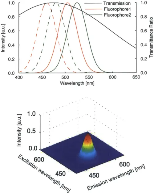
Fluorescence EEMs of samples containing several fluorophores in a light-absorbing medium are generated based on Equation 2.2 in MATLAB. Fluorescence excitation and emission spectra are simulated as Gaussians with its peak position pA, and vari-ance o- (n = 1 ... N), .A(po). Since the shape of fluorescence spectra is not important in our algorithm, all of the variances a are set to be equal. An absorption spectrum is also simulated as a Gaussian which has more variance than fluorescence spectra.
As a standard dataset for the performance evaluations, the following parameters are used for the generation of the spectroscopic data: the ground truth spectra are simulated with 1 nm resolution, the sampling bandwidth for excitation and emission spectra measurements is set to be 5 nm, the number of fluorophores N is set to be
2, Apn = Pn - Pn =12 nm for both excitation and emission spectra and a- = 20.
The variance of the absorption spectrum is set to be 1202. The standard dataset is shown in Figure 2-2.
2.3.2
Performance Analysis
To quantify the error of the estimated contributions from each fluorophore, we define the normalized mean squared error (NRMSE) for the estimation of the contributions:
2 c2 / 2
NRMSE =
C
. (2.17)11'||2 l|C 112 2 lIC 112 2
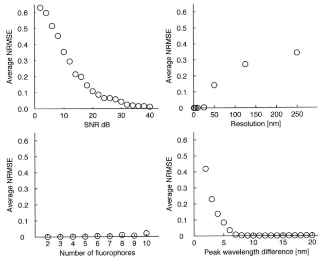
For each evaluation, the average NRMSE was calculated from thirty trials. The parameters for generating datasets are changed for the performance evaluations in the following ways; 1) White Gaussian noise is added to the standard dataset to generate a range of SNR. 2) Sampling resolution for both excitation and emission channels is changed from 1 nm to 250 nm. 3) Api is changed from 1 nm to 20 nm. 4) The number of fluorophores is increased from 2 to 10. All Api is set to be equal. Their spectra are set to be in the range of sampling range.
Transmission -Fluorophorel Fluorophore2 -II \ \ -II\ -\ -\ -a 450 500 550 Wavelength [nm] 600 650
1.0
0.51
0.0 0600
450
600
450
6*
Figure 2-2: Simulated fluorescence emission and excitation spectra and an absorption spectrum (top) and an EEM distorted by the absorption (bottom). Continuous lines are emission spectra, and dotted lines are excitation spectra. The contribution from both fluorophores are simulated to be the same.
0.8 o cc 0.6 0.4 E ca 0.2 0.0 0.8 cd 0.6 0.4 0.2 U.0 400 Cd a) .-. 1.0 1.0
0 0 0 0 0 0 0.6 0.5 0.4 0.3 0.2 0.1 0.0 30 40 w z CD CU a, ,i% ~ ~ n n.-~ ( ) L CD) 2 c CD Ca 0.6 0.5 0.4 0.3 0.2 0.1 0 0.6 0.5 0.4 0.3 0.2 0.1 0 0 0 50 100 150 200 250 Resolution [nm] -0 0 0 2 3 4 5 6 7 8 9 10 0 5 10 15 20
Number of fluorophores Peak wavelength difference [nm]
Figure 2-3: Performance evaluation of NFMU. Normalized root mean squared error of the estimated contributions. The robustness of NFMU is evaluated with SNR, sampling resolution, number of fluorophores and peak wavelength difference.
Figure 2-3 summarizes the performance of our proposed method. As SNR and sampling rate increases, the proposed method estimates the contribution ratio accu-rately. Since the standard dataset has 5 nm resolution for excitation and emission channels, the performance degrades when the peak wavelength difference is less than
5 nm. Remarkably, the number of fluorophores does not affect the estimation error.
2.3.3
Generation of Spectral Imaging Datasets
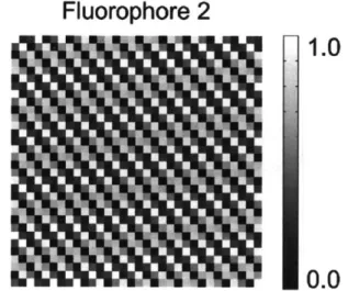
As in spectroscopy, excitation and emission spectra and an absorption spectrum are simulated in the same way. In a 32 by 32 pixel image, each fluorophore is simulated to have different spatial distributions. Their distribution patterns are generated by w CD) CM Ca U) C) CO 0 10 20 SNR dB 0.6 0.5 0.4 0.3 0.2 0.1 0 0 0
O
mr
I
Fluorophore
1
Fluorophore 2
1.0
Figure 2-4: Representative images of simulated fluorophore distributions. The bar shows each fluorophore's abundance.
using the real part of the two dimensional discrete Fourier component. The represen-tative examples of the simulated distributions are shown in Figure 2-4. Commonly, a fluorescence laser scanning microscope is equipped with several excitation lasers whose wavelength are set to be 40 nm apart. To increase signal to noise ratio, the emission channel's bandwidth is set to be 10 nm in spectral imaging mode. The standard dataset for spectral imaging is simulated in such a way.
2.3.4
Performance Analysis
Similarly to the evaluation of the fluorescence spectroscopy, the NRMSE is defined as follows:
NRMSE= T -T/ . (2.18)
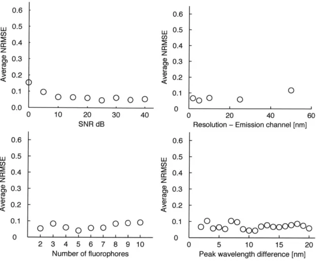
Here, T and T are a row-wise normalized matrix of T and T, respectively. For each evaluation, the average NRMSE was calculated from ten trials. Similarlly to the simulation of fluorometer, the parameters for generating datasets are changed from the standard spectral imaging dataset for the performance evaluations in the following ways: 1) White Gaussian noise is added to the standard dataset to generate a range of SNR. 2) Sampling resolution for both excitation and emission channels is
0.6 W 0.5 a0.4 0.3 Ca 0.2 0.1 0 CD, C) Ca U) w a) (M CU a) 0.6 0.5 0.4 0.3 0.2 0.1 0.0 0.6 0.5 0.4 0.3 0.2 0.1 n 0 0 10 20 SNR dB 30 40 w 2 z a: 0) CO 0 0 00000
0
000 0 0.6 0.5 0.4 0.3 0.2 0.1 0 0 20 40Resolution - Emission channel [nm] 60
- 000
oo000000
O0V
2 3 4 5 6 7 8 9 10 0 5 10 15 20
Number of fluorophores Peak wavelength difference [nm]
Figure 2-5: Performance evaluation of NFTU. Normalized root mean squared error of the estimated contributions in various conditions. The robustness of NFTU is eval-uated with SNR, sampling resolution, number of fluorophores and peak wavelength difference.
changed from 1 nm to 50 nm. 3) Api is changed from 1 nm to 20 nm. 4) The number of fluorophores is increased from 2 to 10. Api is set to be all equal. Their spectra are set to be in the range of sampling range.
Figure 2-5 summarizes the performance of NTFU in terms of the estimation error of molecular fractions. As can be seen, NTFU is robust to all of the four parameters. Even though the spectral resolution of emission wavelength is 10 nm, NTFU can accurately estimate the fractions of fluorophores whose spectra are highly overlapping.
C
0
2.4 Experimental Results
2.4.1
Fluorometer
Fluorescence solution was prepared by dissolving two fluorophores, disodium fluores-cein and 4-(Dicyanomethylene)-2-methyl-6-(4-dimethylaminostyryl)-4H-pyran (pyrene derivative), in ethanol. Green ink in a commercial pen was used as light absorbent. The EEMs of samples were measured with a conventional fluorescence spectropho-tometer at room temperature. The reference excitation and emission spectra of each fluorophore were obtained separately. By using these reference spectra, NFMU and
LU were applied to the EEMs of the mixtures to estimate the molecular fraction.
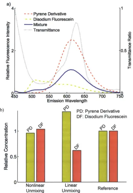
The proposed NFMU and the linear unmixing algorithm were applied to the mea-sured fluorescence EEMs. The estimated contribution ratios of the two fluorophores were compared with the ground truth (Figure 2-6). As is clearly seen, NFMU accu-rately estimated the contribution ratio, as opposed to linear unmixing.
2.4.2 Fluorescence Microscopy
The FocalCheck fluorescence Microscope Test Slide #2 (Life Technologies), which is commonly used for testing linear unmixing algorithm, was used as a sample. The test slide contains microspheres. Their shell and core are stained with different fluo-rophores whose fluorescence spectra are significantly overlapping. The emission spec-tra are shown in Figure 2-7. Images were captured by a Zeiss LSM 710 laser scan-ning confocal microscope with 488 nm and 514 nm excitation lasers. The emission wavelength bandwidth was set to be 10 nm. A Plan-Apo 63x/1.4 NA oil immersion objective was used. The size of a pinhole was set to 1 airy unit.
To imitate the environment of deep tissue imaging, hemoglobin from bovine blood was used as fluorescence attenuator. Lyophilized powder of hemoglobin was dissolved in distilled water and placed on a coverslip. After evaporation of the solution, the coverslip was placed on each sample. Then, the image was captured through the two stacked coverslips. Although the objective is not designed to capture images
a) 4 1 - - - Pyrene Derivative Disodium Fluorescein - Mixture -. Transmittance E 50 500 550 600 650 700 751S Emission Wavelength b) PD: Pyrene Derivative DF: Disodiumn Fluorescein "ii*-0 0.5-WI Nonlinear Lineare Unmixing UnmixingRfrnc
Figure 2-6: Experimental result of fluorometer. (a) Measured emission spectra of 4-(Dicyanomethylene)-2-methyl-6-(4-dimethylaminostyryl)-4H-pyran, Disodium
Flu-orescein, and the mixture of the two fluorophores with absorbent and the absorption spectrum of the absorbent. The fluorescence spectra are measured with the right-angle geometry. The excitation wavelength is 400 nm. Ethanol is used as a solvent. (b) Comparison of estimated relative concentrations and reference concentrations of each type of the fluorophores. The concentrations are estimated by the developed
nonlinear unmixing and the conventional linear unmixing algorithms.
through two coverslips, oil immersion objectives can capture sharp images without suffering from spherical abberation because immersion oil is designed to have the same refractive index to glass coverslips. Then, NFTU and LU were applied to the
1 > 0.8 C - 0.6 N E 0.4 0
z
0.2 0 - Fluorophore 1 (Core) -A Fluorophore 2 (Shell) 500 530 560 590 Emission wavelength [nm] 620Figure 2-7: Emission spectra of the microsphere's fluorophores, measured with con-focal microscopy.
spectral images.
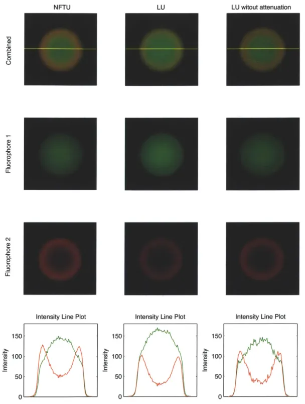
Fig. 2-8 shows the images of the microspheres unmixed by LU and NFTU. Since the microspheres are stained with different fluorophores at its core and shell, the fluorescence light from Fluorophore 2 should dominate at the shell, which is seen in the LU-unmixed images captured without hemoglobin. However, the LU-unmixed images captured through hemoglogin do not show the dominance of Fluorophore 2 on the shell. On the other hand, the NFTU-unmixed images clearly show the dominance of the Fluorophore 2 on the shell. The signals both at the core and the shell has contribution from both fluorophores because of out-of-focus light.
2.5 Discussion
2.5.1
Benefits and Limitations
In summary, we have presented new nonlinear fluorescence unmixing algorithms,
use multiplicative update rules for nonnegative matrix and tensor factorization. From a EEM measurement of a sample, NFMU estimates the abundance of fluorophores by using each fluorophore's EEM. On the other hand, NFTU unmixes spectral images of a multiply-stained sample acquired with several excitation wavelengths by using only emission spectra of flurophores. To the best of our knowledge, NFTU is the only unmixing algorithm which separates fluorescence spectral images affected by absorp-tion. Although we showed the performance of both NFMU and NFTU on samples containing two fluorophores in experiments, they can be applied to unmix spectra of samples containing more than two fluorophores, as we show in the simulation.
NFTU is a natural extension of NFMU. However, in contrast to NFMU, NFTU
exploits the benefit of large number of samples in one image acquisition. By utilizing this advantage, NFTU is much more robust to noise compared to NFMU.
NFMU and NFTU have several limitations inherent to EEM measurements and
fluorescence spectral imaging. Since both methods require scanning of wavelength with narrow bandwidth, there is an inevitable trade-off between scanning time, noise level and sampling resolution. Since this trade-off depends on the properties of flu-orophores, an optimization framework for finding the best measurement parameters should be developed. In addition, as is the case with SU and PARAFAC, NFMU and
NFTU cannot be applied when fluorescence spectral properties change due to other
nonlinearities, such as quenching and pH dependence [17].
2.5.2
Future Work
While our algorithms, NFMU and NFTU, require spectral information of fluorophores as a priori knowledge, we would like to explore a new mathematical technique for blind unmixing of our fluorescence model 2.2 and 2.11. As is incorporated in several blind unmixing methods [34, 35], fluorescence lifetime would help to solve the problem. Fur-thermore, the evaluation of NFMU should be compared with existing inner-filtering correction methods. While we examined our algorithms on experimentally-controlled samples, we would like to apply our methods, NFMU and NFTU, to real world prob-lems, such as the analysis of dissolved organic matter and deep tissue imaging.
LU witout attenuation E 0 0 C) 0. 0 CLJ 0 :3 150
Intensity Line Plot
0, C U) C 150 100' 501 0 2:.Cr 5, a 150 100 50 0
Intensity Line Plot
Figure 2-8: Unmixed images of microspheres stained with two fluorophores. The left and middle column show the unmixed results on the same spectral image datasets captured through hemoglobin. The right column shows the unmixed results by LU on the datasets captured without hemoglobin. The top row shows the combined image
of the second and third row. The bottom row shows the contribution from each
fluorophore on the yellow line of the top-row images. Colors are pseudocolor.
Intensity Line Plot
cn C U) C 100 50 0 NFTU LU
Chapter 3
Switchable Multiple Oblique
Illumination Microscopy
3.1
Proposed Method and Related Work
Surface roughness in microscopic scale is an important characteristic of materials. To characterize it, various optical methods have been developed, such as confocal mi-croscopy [36], fringe projection
[37]
and interferometry[381.
There are also more ac-curate non-optical methods available, including scanning electron microscopy (SEM) and atomic force microscopy (AFM). Among them, microscopic photometric stereo is one of the easiest and cheapest methods for 3D measurement of microscopic structure[39]. With a conventional long-working distance microscope, this method captures
several microscopic images with manually-changed illumination directions and applies the photometric stereo method to extract surface albedos, surface normals and height of microstructure. Even though it is easy-to-implement, this method only shows the structures more than several micrometers due to diffraction of light. However, there is a need in many fields, such as defect inspection and dermatology, for a method that can visualize the surface microstructure as small as the illumination wavelength with an easily-implementable device, instead of accurately measuring the roughness. We introduce such a method here.
multi-ple light sources to a reflected light compound microscope. Oblique illumination is
a traditional technique in transmission light microscopy to enhance image contrast.
It is also applied to endoscopy to obtain phase-gradient images [40]. Although this
microscope, called oblique back-illumination microscopy, configures epi-illumination geometry, the light collected by an objective lens transmits through tissue like trans-illumination geometry. As often used in reflected-light stereomicroscopy, oblique illumination can reveal surface structures much smaller than the illumination
wave-length [36]. In addition, the angle of illumination relative to both a sample and the
optical axis is also of great importance to increase image contrast. However, to the
best of our knowledge, the capability of oblique illumination with reflected-light
com-pound microscopy has not been explored yet. In particular, we make the following contributions:
. We build the prototype of the switchable multiple oblique illumination
com-pound microscope system in reflection mode.
. We examined its performance by acquiring images of microscopic features as small as the illumination wavelength.
3.2 Method
This section describes the switchable oblique reflected illumination microscopy which qualitatively assess the surface roughness.
3.2.1
Hardware Implementation
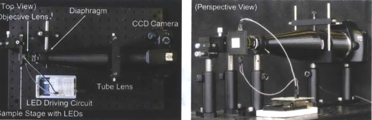
The hardware is composed of Canon's EOS Rebel T3 digital camera, Olympus's UPlanSApo 20x NAO.75 objective lens and tube lens, a No.1.5 coverslip, an iris
di-aphragm (00.8 to 020 mm), Arduino Mega with a light-emissing diode (LED) driving
circuit, a XYZ translation stage and 3D printed light blockers and sample stages and white LEDs (Figure. 3-1). The illumination angle is set to be nearly 900 to the optical
Figure 3-1: Prototype of the multiple oblique illumination microscope.
axis of the objective lens (Figure. 3-2). To increase the depth of field, the size of the iris is set to be the smallest size.
Our microscope system is controlled via MATLAB. The LEDs are switchable through serial communication, and the image acquisition is achieved with the cross-platform digital camera library, gPhoto2 [41]. Two images are sequentially acquired with each LED illumination.
3.2.2
Sample Preparation
Intact black hair and bleached and dyed black hair are used as samples. Hair is covered with cuticle cells which consist of the outermost layers. Each cuticle cell has about 500 nm thickness. Since bleaching and coloration dissolve the cell membrane complex that connects cuticles to each other, the cuticles of the bleached and dyed hair is partly ripped off from the surface [42]. The SEM images of intact and damaged hair surface is shown in Figure 3-3. For the image acquisition, a single strand of hair is placed on the custom-designed stage (Figure 3-2).
3.3 Result
Figure 3-5 and 3-6 show the images of the healthy hair and highly-damaged hair illuminated from tip and root side. In the case of black hair, light penetrating the surface is absorbed by the melanin pigment, and subsurface scattered light is negligible
Objective Lens
LED Sample (Hair)
Figure 3-2: A sample stage for a hair strand and a adapter for a translational stage
(left) and a schematic illustration of illuminating direction (right). The sample holder is designed to be inserted to the adapter to the translational stage.
Figure 3-3: Scanning electron micrographs of healthy hair (left) and damaged hair (right), cited from [42].
for the image formation. Therefore, the image-forming light is surface-reflected light. As is illustrated in Figure 3-4, the edge of cuticles of intact hair has higher scat-tering and reflection when illuminated from root. Since the effective roughness for illumination from tip is the thickness of cubicles, incident light from tip strongly scat-ters at the edge of cuticles. On the other hand, in the case of damaged hair, both incident illuminations from tip and root side scatter and reflect strongly at the edge of detached cuticles due to the ripped-off cuticles.
To extract the scattering effect in images, the variance map of the captured images are calculated and shown in Figure 3-5 and 3-6. As can be clearly seen in Figure 3-6,
Healthy Hair Damaged Hair
Illumination
from root side
Illumination
from tip side
&&
Figure 3-4: Illustration of the interaction between the direction of illumination and hair surface. The condition of cuticles affects the reflection and scattering of light.
the computation of local variance enhances the contrast of cuticles and suppresses the undesirable contrast from out-of-focus light. While the healthy hair shows the shape of cuticles in the variance image with the illumination from tip side but not with the illumination from root, the shape of cuticles is revealed in the variance map with both illuminations.
3.4 Discussion
3.4.1
Benefits and Limitations
Taking intact and damaged hair as a representative sample, we show that the switch-able oblique reflected illumination microscope system extracts the anisotropy of sur-face roughness whose height is about the same size as illumination wavelength. While one of the computational photography techniques enhances depth-edge with multiple flashes in macroscopic scale [43], our microscope extracts depth-edge in microscopic
Illuminated from tip Illuminated from root
Figure 3-5: Images of healthy black hair captured by the prototype and their processed images. The top row shows the original microscopic images. The bottom row shows their local variance map. Illumination from root side enhances the contrast at the edge of cuticles. a) CD E 0. 0 C) CO) E C.) Cu
Illuminated from tip Illuminated from root
Figure 3-6: Images of damaged black hair captured by the prototype and their pro-cessed images. The top row shows the original microscopic images. The bottom row shows their local variance map. Illumination from both tip and root side enhances the contrast at the edge of cuticles.
a) 0D Ca E 0 0. 0a 0 CL) Ca) . cc
scale. Compared to the conventional surface probing technologies, our system is re-markably low-cost and small. This simple setup will allow surface diagnostics of materials in resource-limited environment.
Furthermore, our microscopic technique reveals the surface damage of hair. To the best of our knowledge, the detachment of cuticles has been undetectable with optical microscopy. Currently, hair researchers utilize SEM to analyze the surface of hair. However, SEM requires metal-coating for biological specimens, which prevents the observation of samples in intact state. Therefore, a method to characterize the surface structure without artificial procedures on samples has been awaited. Our microscope system has large potential to advance hair research and can be used as a quick hair diagnostic device for consumer applications.
The prototype has several limitations. While AFM and SEM can quantitatively measure the roughness and reveal three dimensional surface structure, our system does not provide quantitative roughness value and elucidate the structure of surface. In addition, subsurface light transport can contribute to the image formation, which may deteriorate the analysis. In this case, the removal of subsurface reflection with an advanced lighting system, such as structured illumination and polarized light, is re-quired. A detailed analysis of the multiple oblique illumination system in comparison to the conventional probing technologies is left for future work.
3.4.2 Future Direction
Our current prototype utilizes a personal computer, a high-quality objective lens and a CCD image sensor of a digital SLR camera. As a next step, we would like to miniaturize it with the use of a smartphone. Since most smartphones have enough computation power and a high resolution image sensor, we plan to develop an attach-ment which modifies a smartphone to a multiple oblique illumination microscope. Furthermore, we currently compute local variance of images after capture. We would like to explore the strategy to quantitatively measure roughness by the co-design of optical system and computation. We believe that the quantitative measurements further expand the application of the switchable multiple oblique illumination.
Chapter 4
Conclusion
Computational control of illumination creates large potential in optical imaging [44,
45, 46]. As opposed to photography, optical microscopy has full control of illumina-tion. This capability has allowed numerous optical designs to acquire different prop-erties of microscopic samples. Even though spectral imaging was introduced to fluo-rescence microscopy about ten years ago and oblique illumination was invented more than three hundred years ago, integration with modern computational approaches had not been explored. In this thesis, we explored the possibilities of fluorescence spectroscopy and microscopy and oblique illumination microscopy.
In science and engineering, not limited to microscopy, a large number of advanced sensing methods have been proposed to measure various material properties. In most cases, however, computational and mathematical analysis of captured data have not been conducted enough to extract information as much as possible. We hope that this thesis inspires others to explore imaging and sensing technologies at the interface of material analysis and computing.
Bibliography
[1] D. B. Murphy and M. W. Davidson, Fundamentals of Light Microscopy and
Electronic Imaging. Wiley-Blackwell, 2 ed., Oct. 2012.
[2] S. Inoue, Video microscopy : the fundamentals. New York: Plenum Press, 1997.
[3] K. Marwah, G. Wetzstein, Y. Bando, and R. Raskar, "Compressive light field
photography using overcomplete dictionaries and optimized projections," ACM
Transactions on Graphics, vol. 32, pp. 46:1-46:12, July 2013.
[4] A. Velten, T. Willwacher, 0. Gupta, A. Veeraraghavan, M. G. Bawendi, and R. Raskar, "Recovering three-dimensional shape around a corner using ultrafast time-of-flight imaging.," Nature communications, vol. 3, p. 745, 2012.
[5] D. Lanman, G. Wetzstein, M. Hirsch, W. Heidrich, and R. Raskar, "Polarization
fields: Dynamic light field display using multi-layer lcds," ACM Transactions on
Graphics, vol. 30, pp. 186:1-186:10, Dec. 2011.
[6] X. Lin, J. Suo, G. Wetzstein,
Q.
Dai, and R. Raskar, "Coded focal stack pho-tography," in IEEE International Conference on Computational Photography,pp. 1-9, April 2013.
[7] R. Raskar, A. Agrawal, and J. Tumblin, "Coded exposure photography: Motion
deblurring using fluttered shutter," ACM Transactions on Graphics, vol. 25,
pp. 795-804, July 2006.
[8] M. Shribak and R. Oldenbourg, "Techniques for fast and sensitive
measure-ments of two-dimensional birefringence distributions.," Applied Optics, vol. 42,
pp. 3009-3017, June 2003.
[9] M. Shribak, "Quantitative orientation-independent differential interference
con-trast microscope with fast switching shear direction and bias modulation," J.
Opt. Soc. Am. A, vol. 30, pp. 769-782, Apr 2013.
[10] M. G. Gustafsson, "Surpassing the lateral resolution limit by a factor of two using
structured illumination microscopy.," Journal of microscopy, vol. 198, pp. 82-87, May 2000.
[11] M. J. Rust, M. Bates, and X. Zhuang, "Sub-diffraction-limit imaging by
stochas-tic opstochas-tical reconstruction microscopy (STORM).," Nature methods, vol. 3,
pp. 793-795, Oct. 2006.
[12] E. Betzig, G. H. Patterson, R. Sougrat, 0. W. Lindwasser, S. Olenych, J. S. Bonifacino, M. W. Davidson, J. Lippincott-Schwartz, and H. F. Hess, "Imaging intracellular fluorescent proteins at nanometer resolution.," Science, vol. 313,
pp. 1642-1645, Sept. 2006.
[13] J. Zhang, S.-Z. Liu, J. Yang, M. Song, J. Song, H.-L. Du, and Z.-P. Chen,
"Quan-titative spectroscopic analysis of heterogeneous systems: chemometric methods for the correction of multiplicative light scattering effects : Reviews in Analytical Chemistry," Reviews in Analytical Chemistry, vol. 32, no. 2, pp. 113-125, 2013. [14] Y. Garini, I. T. Young, and G. McNamara, "Spectral imaging: Principles and
applications," Cytometry Part A, vol. 69A, no. 8, pp. 735-747, 2006.
[15] R. Neher and E. Neher, "Optimizing imaging parameters for the separation of
multiple labels in a fluorescence image.," Journal of Microscopy, vol. 213, pp.
46-62, Jan. 2004.
[16] T. Zimmermann, J. Marrison, K. Hogg, and P. O'Toole, "Clearing up the signal:
spectral imaging and linear unmixing in fluorescence microscopy.," Methods in
molecular biology, vol. 1075, pp. 129-148, 2014.
[17] K. R. Murphy, C. A. Stedmon, D. Graeber, and R. Bro, "Fluorescence
spectroscopy and multi-way techniques. parafac," Analytical Methods, vol. 5,
pp. 6557-6566, Sept. 2013.
[18] R. S. Bradley and M. S. Thorniley, "A review of attenuation correction techniques
for tissue fluorescence.," Journal of the Royal Society Interface, vol. 3, pp. 1-13, Feb. 2006.
[19] X. Luciani, S. Mounier, R. Redon, and A. Bois, "A simple correction method of
inner filter effects affecting FEEM and its application to the PARAFAC decom-position," Chemometrics and Intelligent Laboratory Systems, vol. 96, pp.
227-238, Apr. 2009.
[20] B. Fanget, 0. Devos, and M. Draye, "Correction of inner filter effect in mirror coating cells for trace level fluorescence measurements.," Analytical Chemistry, vol. 75, pp. 2790-2795, June 2003.
[21] J. C. Finlay and T. H. Foster, "Recovery of hemoglobin oxygen saturation and intrinsic fluorescence with a forward-adjoint model," Applied Optics, vol. 44,
pp. 1917-1933, Apr 2005.
[22] S. Avrillier, E. Tinet, D. Ettori, J. M. Tualle, and B. G616bart, "Influence of the emission-reception geometry in laser-induced fluorescence spectra from turbid media.," Applied Optics, vol. 37, no. 13, pp. 2781-2787, 1998.
[23] D. D. Lee and H. S. Seung, "Learning the parts of objects by non-negative matrix
factorization.," Nature, vol. 401, pp. 788-791, Oct. 1999.
[24] W. Denk, J. H. Strickler, and W. W. Webb, "Two-photon laser scanning fluores-cence microscopy.," Science, vol. 248, pp. 73-76, Apr. 1990.
[25] F. Helmchen and W. Denk, "Deep tissue two-photon microscopy.," Nature
Meth-ods, vol. 2, pp. 932-940, Dec. 2005.
[26] J. Livet, T. A. Weissman, H. Kang, R. W. Draft, J. Lu, R. A. Bennis, J. R.
Sanes, and J. W. Lichtman, "Transgenic strategies for combinatorial expression of fluorescent proteins in the nervous system.," Nature, vol. 450, pp. 56-62, Nov.
2007.
[27] D. Cai, K. B. Cohen, T. Luo, J. W. Lichtman, and J. R. Sanes, "Improved tools
for the Brainbow toolbox.," Nature Methods, vol. 10, pp. 540-547, May 2013.
[28] S. Henrot, C. Soussen, M. Dossot, and D. Brie, "Does deblurring improve
ge-ometrical hyperspectral unmixing?," IEEE Transactions on Image Processing, vol. 23, pp. 1169-1180, March 2014.
[29] J. Wu, M. S. Feld, and R. P. RAVA, "Analytical model for extracting intrinsic
fluorescence in turbid media.," Applied Optics, vol. 32, pp. 3585-3595, July 1993.
[30] M. G. M6ler, I. Georgakoudi,
Q.
Zhang, J. Wu, and M. S. Feld, "Intrinsic fluorescence spectroscopy in turbid media: disentangling effects of scattering and absorption.," Applied Optics, vol. 40, pp. 4633-4646, Sept. 2001.[31] T. G. Kolda and B. W. Bader, "Tensor Decompositions and Applications," SIAM
Review, vol. 51, pp. 455-500, Aug. 2009.
[32] H. Shirakawa and S. Miyazaki, "Blind spectral decomposition of single-cell
fluo-rescence by parallel factor analysis," Biophysical Journal, vol. 86, pp. 1739-1752, Mar. 2004.
[33] G. Wetzstein, D. Lanman, M. Hirsch, and R. Raskar, "Tensor displays:
Compres-sive light field synthesis using multilayer displays with directional backlighting,"
ACM Transactions on Graphics, vol. 31, pp. 80:1-80:11, July 2012.
[34] S. Schlachter, S. Schwedler, A. Esposito, G. S. Kaminski Schierle, G. D. Mog-gridge, and C. F. Kaminski, "A method to unmix multiple fluorophores in mi-croscopy images with minimal a priori information.," Optics Express, vol. 17,
pp. 22747-22760, Dec. 2009.
[35] C. Barsi, R. Whyte, A. Bhandari, A. Das, A. Kadambi, A. A. Dorrington, and
R. Raskar, "Multi-frequency reference-free fluorescence lifetime imaging using a time-of-flight camera," in Biomedical Optics 2014, p. BM3A.53, Optical Society of America, 2014.
[36] J. Mertz, Introduction to Optical Microscopy. Roberts & Company, 2010. [37] C. Zhang, P. S. Huang, and F.-P. Chiang, "Microscopic phase-shifting
profilom-etry based on digital micromirror device technology," Applied Optics, vol. 41,
pp. 5896-5904, Oct 2002.
[38] Z. Li and Y. Li, "Gamma-distorted fringe image modeling and accurate gamma
correction for fast phase measuring profilometry," Optics Letters, vol. 36, pp.
154-156, Jan 2011.
[39] Z. Li and Y. Li, "Microscopic photometric stereo: A dense microstructure 3d
measurement method," in IEEE International Conference on Robotics and
Au-tomation, pp. 6009-6014, May 2011.
[40] T. N. Ford, K. K. Chu, and J. Mertz, "Phase-gradient microscopy in thick tissue with oblique back-illumination," Nature Methods, vol. 9, pp. 1195-U90, Dec.
2012.
[41] "gPhoto Website." http://gphoto.sourceforge.net/, 2014.
[42] C. R. Robbins, Chemical and Physical Behavior of Human Hair. Springer, 5th edition ed., Feb. 2012.
[43] R. Raskar, K.-H. Tan, R. Feris, J. Yu, and M. Turk, "Non-photorealistic camera: Depth edge detection and stylized rendering using multi-flash imaging," ACM
Transactions on Graphics, vol. 23, pp. 679-688, Aug. 2004.
[44] A. Kadambi, R. Whyte, A. Bhandari, L. Streeter, C. Barsi, A. Dorrington, and R. Raskar, "Coded time of flight cameras: Sparse deconvolution to address mul-tipath interference and recover time profiles," ACM Transactions on Graphics, vol. 32, pp. 167:1-167:10, Nov. 2013.
[45] A. Bhandari, A. Kadambi, R. Whyte, C. Barsi, M. Feigin, A. Dorrington, and R. Raskar, "Resolving multipath interference in time-of-flight imaging via mod-ulation frequency diversity and sparse regularization," Optics Letters, vol. 39,
pp. 1705-1708, Mar 2014.
[46] D. Wu, M. O'Toole, A. Velten, A. Agrawal, and R. Raskar, "Decomposing global light transport using time of flight imaging," in IEEE Conference on Computer