HAL Id: hal-03145271
https://hal.archives-ouvertes.fr/hal-03145271
Submitted on 18 Feb 2021
HAL is a multi-disciplinary open access
archive for the deposit and dissemination of
sci-entific research documents, whether they are
pub-lished or not. The documents may come from
teaching and research institutions in France or
abroad, or from public or private research centers.
L’archive ouverte pluridisciplinaire HAL, est
destinée au dépôt et à la diffusion de documents
scientifiques de niveau recherche, publiés ou non,
émanant des établissements d’enseignement et de
recherche français ou étrangers, des laboratoires
publics ou privés.
Statistical Survey of the Terrestrial Bow Shock
Observed by the Cluster Spacecraft
O. Kruparova, V. Krupar, J. Šafránková, Z. Němeček, M. Maksimovic, O.
Santolik, J. Soucek, F. Němec, J. Merka
To cite this version:
O. Kruparova, V. Krupar, J. Šafránková, Z. Němeček, M. Maksimovic, et al.. Statistical Survey of the
Terrestrial Bow Shock Observed by the Cluster Spacecraft. Journal of Geophysical Research Space
Physics, American Geophysical Union/Wiley, 2019, 124 (3), pp.1539-1547. �10.1029/2018JA026272�.
�hal-03145271�
O. Kruparova1 , V. Krupar1,2,3 , J. Šafránková4 , Z. Nˇemeˇcek4 , M. Maksimovic5,
O. Santolik1,4 , J. Soucek1 , F. Nˇemec4 , and J. Merka3,6
1Department of Space Physics, Institute of Atmospheric Physics, The Czech Academy of Sciences, Prague, Czech
Republic,2Universities Space Research Association, Columbia, MD, USA,3NASA Goddard Space Flight Center,
Greenbelt, MD, USA,4Faculty of Mathematics and Physics, Charles University, Prague, Czech Republic,5LESIA,
Observatoire de Paris, Université PSL, CNRS, Sorbonne Université, University Paris Diderot, Sorbonne Paris Cité, Meudon, France,6Goddard Planetary Heliophysics Institute, University of Maryland, Baltimore County, Baltimore,
MD, USA
Abstract
The terrestrial bow shock provides us with a unique opportunity to extensively investigate properties of collisionless shocks using in situ measurements under a wide range of upstream conditions. Here we report a statistical study of 529 terrestrial bow shock crossings observed between years 2001 and 2013 by the four Cluster spacecraft. By applying a simple timing method to multipoint measurements, we are able to investigate their characteristic spatiotemporal features. We have found a significant correlation between the speed of the bow shock motion and the solar wind speed. We have also compared obtained speeds with time derivatives of locations predicted by a three-dimensional bow shock model. Finally, we provide a list of bow shock crossings for possible further investigation by the scientific community.Plain Language Summary
The Sun is continuously emitting a stream of charged particles—called the solar wind—from its upper atmosphere. The terrestrial magnetosphere forms the obstacle to its flow. Due to supersonic speed of the solar wind, the bow shock is created ahead of the magnetosphere. This abrupt transition region between supersonic and subsonic flows has been frequently observed by the four Cluster spacecraft. Using a timing analysis, we have retrieved speed and directions of the bow shock motion for a large number of crossings. We have correlated the bow shock speed with the solar wind speed and predictions of the bow shock locations by the empirical model. A better understanding of the bow shock kinematics may bring new insights to wave-particle interactions with applications in laboratory plasmas.1. Introduction
Collisionless shocks represent a special case of shock waves where the transition between the upstream and downstream regions is present on a length scale much smaller than a particle collisional mean free path. The terrestrial bow shock is formed by a continuous interaction between the supersonic solar wind and Earth's magnetic field (Eastwood et al., 2015; Tsurutani et al., 2011). It has been intensively studied over the last few decades from both theoretical and experimental standpoints (e.g., Parks et al., 2017, and references therein). Spreiter et al. (1966) introduced an Magnetohydrodynamic (MHD) model of the interaction between the solar wind and the magnetosphere. Since then, various models of the bow shock shape and location have been developed (Farris & Russell, 1994; Formisano, 1979; Jeˇráb et al., 2005; Merka et al., 2005; Peredo et al., 1995). These models are statistically derived from large data sets of bow shock crossings and upstream solar wind parameters.
Nemecek et al. (1988) studied bow shock dynamics using simultaneous measurements by the Prognoz 10 and IMP-8 spacecraft. They observed a correlation between the bow shock speed and deviations from the modeled bow shock locations predicted by Formisano (1979). Šafránková et al. (2003) analyzed ∼130 bow shock crossings observed by the Interball-1 and Magion-4 spacecraft pair—regardless of upstream parame-ters, geometry, and𝜃Bn(the angle of the upstream magnetic field to the bow shock normal)—and found that
the bow shock velocities in the spacecraft frame range from 0 to 100 kms−1, but a majority of them (78%) is
less than 40 kms−1.
Key Points:
• A significant correlation between the speed of the bow shock motion and the solar wind speed has been found • Relative deviations from the model
bow shock location are correlated with the bow shock speed • The list of bow shock crossings
observed by the four Cluster spacecraft between years 2001 and 2013 is provided as an Auxiliary material Supporting Information: • Supporting Information S1 • Data Set S1 Correspondence to: O. Kruparova, [email protected] Citation:
Kruparova, O., Krupar, V., Šafránková, J., Nˇemeˇcek, Z., Maksimovic, M., Santolik, O., et al. (2019). Statistical survey of the terrestrial bow shock observed by the Cluster spacecraft. Journal of
Geophysical Research: Space Physics, 124.
https://doi.org/10.1029/2018JA026272
Received 12 NOV 2018 Accepted 10 FEB 2019
Accepted article online 13 FEB 2019
©2019. American Geophysical Union. All Rights Reserved.
Journal of Geophysical Research: Space Physics
10.1029/2018JA026272
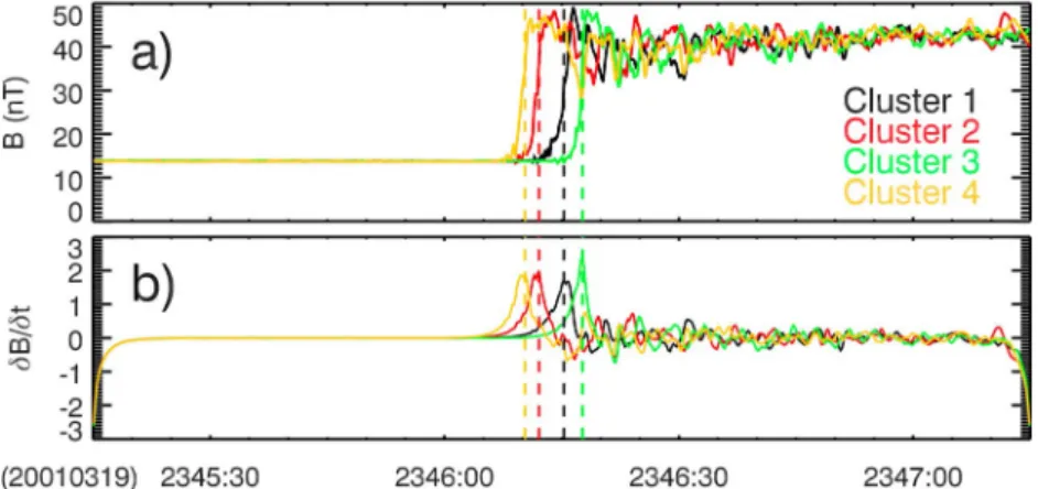
Figure 1. An example of a bow shock crossing observed on 19 March 2001. (a) The magnetic field magnitude and
(b) its first time derivatives are displayed for four Cluster spacecraft. The dashed color lines correspond to the shock crossing times for a particular spacecraft.
Recent multipoint measurements recorded by the four Cluster spacecraft allow us to investigate spatiotem-poral variations of the terrestrial bow shock under different upstream conditions for a long period of time. We are listing several preceding studies that are dedicated to bow shock kinematics using a timing method applied to Cluster observations hereafter. We note that bow shocks are classified as quasiperpendicular and quasiparallel according to whether𝜃Bnis greater or less than 45◦, respectively. Horbury et al. (2002)
inves-tigated 48 quasiperpendicular bow shocks from 2000 to 2001. They found that the bow shock speed in the spacecraft frame is typically ∼35 kms−1. Maksimovic et al. (2003) studied a series of 11 consecutive bow
shock crossings observed on 31 March 2001 by Cluster. These bow shock oscillations were comparable with the predictions by the Farris and Russell (1994) gasdynamic model. Meziane et al. (2014) investigated the shape and motion of the bow shock based on 133 bow shock crossings. Meziane et al. (2015) analyzed 381 individual bow shock crossings between years 2000 and 2002. Using averaged solar wind conditions during this period, they concluded that the ram pressure is a predominant parameter of the bow shock dynamics.
Recently, Mejnertsen et al. (2018) performed global MHD simulations of bow shock oscillations from 31 March 2001 using the upstream data retrieved by the Advanced Composition Explorer (ACE) spacecraft. This day was previously analyzed by Maksimovic et al. (2003). They found that the standard deviations of the simulated bow shock motion are 17.7 and 26.6 kms−1in the subsolar region (<45◦from X axis) and the
flanks (>45◦from X axis), respectively.
In this paper, we examine statistical properties of the terrestrial bow shock with a focus on its kinematics. In section 2, we show an example of a bow shock crossing to demonstrate our analysis and a method of bow shock crossing identification. In section 3, we investigate bow shock speeds and locations. Finally, the summary and conclusions are listed in section 4.
2. Data Analysis
We have investigated a large number of bow shock crossings between years 2001 and 2015 observed by the four Cluster spacecraft (Escoubet et al., 2001). During this period, the Cluster mission accumulated a substantial set of multipoint measurements covering a wide range of the bow shock area under various upstream conditions. For the bow shock identification, we primarily analyzed magnetic field and plasma measurements recorded by the Flux Gate Magnetometer and Cluster Ion Spectrometry-Hot Ion Analyzer (CIS-HIA) instrument, respectively (Balogh et al., 2001; Rème et al., 2001). The Cluster data were retrieved from the Cluster Science Archive (Laakso et al., 2010). We have excluded from our analysis periods when the ratio between the largest and smallest spacecraft separation distances was larger than 20, and temporal differences between bow shock measurements at four spacecraft was smaller than 1 s.
As an example from our list of events, we show an analysis of a bow shock crossing from 19 March 2001 when the four Cluster spacecraft were located at (13.4, − 1.1, 8.4) REin the Geocentric Solar Ecliptic coordinate
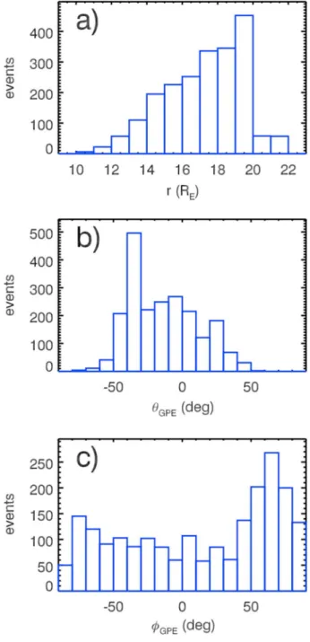
Figure 2. (a)–(c) Cluster spacecraft locations in the GPE spherical
coordinate system. GPE = Geocentric Plasma Ecliptic.
We can identify an abrupt jump from 15 to 45 nT at approximately 23:46:15 UT detected by all spacecraft during their transition from the solar wind to the magnetosheath. We also observe a characteris-tic increase of magnecharacteris-tic field fluctuations in the downstream of the bow shock. Variations in plasma parameters recorded by CIS-HIA con-firm that the Cluster spacecraft crossed the bow shock at that moment (abrupt jumps in both density and bulk speed; not shown here). Due to instrumental issues, we used plasma measurements by Cluster-1 only to retrieve upstream conditions. We used 5-min averages of the Flux Gate Magnetometer and CIS-HIA data near the bow shock to quantify bow shock properties. The upstream magnetosonic Mach number was 3 in this case.
We use the timing method to determine bow shock normals and velocities along these normals (Horbury et al., 2002; Schwartz, 1998). We assume that a bow shock can be represented by a moving plane with a constant velocity, when observed at closely separated four points in space and time. With the information on a bow shock normal, we can also directly retrieve
𝜃Bn. For a precise identification of bow shock crossing times, we calculate
a numerical derivative of the magnetic field𝛿B∕𝛿t (Figure 1b). We apply the low-pass Butterworth filter at 0.55 Hz to improve the signal-to-noise ratio of𝛿B∕𝛿t. Next, we identify the maximum of 𝛿B∕𝛿t to retrieve times
tiand consequently locations (xi, yi, zi)of the bow shock crossing for each spacecraft separately (denoted by dashed lines in Figure 1a). The bow shock identification is done automatically within a preselected short time interval (2 min in this case; 23:45:15–23:47:15). With this information, we can solve the following equation:
⎛ ⎜ ⎜ ⎜ ⎜ ⎜ ⎜ ⎜ ⎝ x1−x2 𝑦1−𝑦2 z1−z2 x1−x3 𝑦1−𝑦3 z1−z3 x1−x4 𝑦1−𝑦4 z1−z4 x2−x3 𝑦2−𝑦3 z2−z3 x2−x4 𝑦2−𝑦4 z2−z4 x3−x4 𝑦3−𝑦4 z3−z4 ⎞ ⎟ ⎟ ⎟ ⎟ ⎟ ⎟ ⎟ ⎠ ⎛ ⎜ ⎜ ⎜ ⎝ nSCx vSC nSC𝑦 vSC nSCz vSC ⎞ ⎟ ⎟ ⎟ ⎠ = ⎛ ⎜ ⎜ ⎜ ⎜ ⎜ ⎜ ⎜ ⎝ t1−t2 t1−t3 t1−t4 t2−t3 t2−t4 t3−t4 ⎞ ⎟ ⎟ ⎟ ⎟ ⎟ ⎟ ⎟ ⎠ , (1)
where (nSCx, nSCy, andnSCz)is the bow shock normal and vSCrepresents
the speed along this normal in the spacecraft frame. We used the sin-gular value decomposition method to solve the overdetermined set of equations (1). We note that previous studies employ timing analysis method based on a determined linear system with a reference satellite (Horbury et al., 2002; Maksimovic et al., 2003; Meziane et al., 2014, 2015). In the case of the reference satellite, the inversion results depend on this choice of the reference spacecraft. Using the overdetermined systems, we treat all spacecraft contributions equally, and singular value decomposi-tion provides us with robustness needed for this timing method. The best solution for this example (in the sense of minimum sum of squares of differences) is nSC =
(−0.90, 0.01, −0.43) and vSC = 54.5kms−1. Next, we calculated an average speed vector of four
Clus-ter satellites vCL to correct our results to a spacecraft constellation speed. Then we obtain the bow
shock speed in the terrestrial frame vBS = nSCvSC − vCL. Finally, the bow shock normal n is
defined as vBS∕|vBS|. This way we retrieved the bow shock normal n = ( − 0.91, 0.02, − 0.41) and the speed along this normal vBS = 55.6kms−1 in the Geocentric Solar Ecliptic coordinate system (i.e., in the terrestrial frame). By comparing the bow shock normal n with the magnetic field direc-tion B in the upstream, we found that 𝜃Bn is equal to 84.96◦ confirming that the observed bow shock
is nearly perpendicular. We have also compared 𝜃Bn obtained with the timing method with those
obtained using the magnetic coplanarity (𝜃mc
Bn = 86.26◦) and the mixed mode (𝜃
mm
Bn = 86.29◦) methods
Journal of Geophysical Research: Space Physics
10.1029/2018JA026272
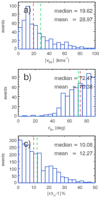
Figure 3. Statistical study of the bow shock properties. (a) Distribution of
the bow shock speed vBS, (b) angle between the bow shock normal and the magnetic field in the upstream𝜃Bn, and (c) absolute value of relative spatial bow shock model deviations. Red and green dashed lines denote mean and median values, respectively.
between these three methods are negligible and below expected precision of the timing analysis in this case.
3. Statistical Results
We have visually identified 1,943 bow shock crossing intervals observed by the four Cluster spacecraft between years 2001 and 2015. Next, we have analyzed only events with an abrupt change in the magnetic field mag-nitude, when an automated determination of shock parameters could be reasonably employed. This constraint results in 529 quasiperpendicular and oblique bow shock intervals only to be included in this study, since a precise identification of times of quasiparallel bow shock crossings is not possible. These events occurred between years 2001 and 2013. We performed the aforementioned analysis on this data set that represents 2,116 individual bow shock crossings as seen by each Cluster spacecraft (i.e., 529 × 4 = 2, 116 events). Figure 2 shows Cluster spacecraft locations in Geocentric Plasma Ecliptic (GPE) coordinate system in which the solar wind velocity is purely radial (Merka & Szabo, 2004). We observed bow shock crossings at radial distances from the Earth r ranging from 10 REto
22 RE(Figure 2a). The cutoff at high radial distance is caused by the space-craft apogee. Majority of our events were located below the ecliptic plane (𝜃GPE < 0; Figure 2b). This asymmetry can be explained by the highly
elliptical spacecraft orbit with an inclination that preferentially covers dayside bow shock regions below the ecliptic and magnetotail above the ecliptic. However, we observed considerably more events on the dusk side of the magnetosphere (𝜙GPE > 0; Figure 2c). It can be expected due to a prevailing interplanetary magnetic field direction following the Archimedean spiral (Parker, 1965) that favors a quasiperpendicular bow shock to be located on the dusk side, while quasiparallel bow shocks are more frequently observed on the dawn side of the magnetosheath (Tsurutani & Rodriguez, 1981).
Figure 3a shows a distribution of the bow shock speed vBS. We have found
that the bow shock has a median speed of ∼20 kms−1, but the
distribu-tion of obtained values has a long tail, with 10% of cases above 63 kms−1.
Our results are comparable to previous statistical studies of Cluster obser-vations performed by Horbury et al. (2002) and (Meziane et al., 1972, 2015). Surprisingly, we have not observed any significant variations of
vBSbetween periods of low and high solar activities (the sunspot
num-ber ranged from 0 in 2008 to ∼250 in 2001). However, differences in the upstream conditions between solar maximum and solar minimum lie essentially in the average values of the solar wind parameters, such as the velocity or the interplanetary magnetic field strength, and in the number of solar transients (e.g., Richardson & Cane, 2012). Generally, during solar minima, coronal holes form long-lived corotating interaction regions which are associated with highly fluctuating solar wind param-eters (Tsurutani et al., 1995). Therefore, the absence of link with the solar cycle may only be due to the fact that solar wind conditions are always dynamic and that the bow shock never reaches an equilibrium position and continuously moves to adjust to changing upstream conditions. We calculated the bow shock median speed for the subsolar region (16.87 kms−1) and the flanks (20.73 kms−1). However, when the speed
is normalized to the radial distance from the Earth, the variation between the subsolar regions and flanks becomes negligible.
Figure 3b shows a distribution of the upstream𝜃Bn. The majority of events in our data set can be classified as quasiperpendicular bow shocks due to our constraint on abruptness of the magnetic field change. We do not observe any correlation between the bow shock speed and𝜃Bn. Note that𝜃Bnuses the normal direction
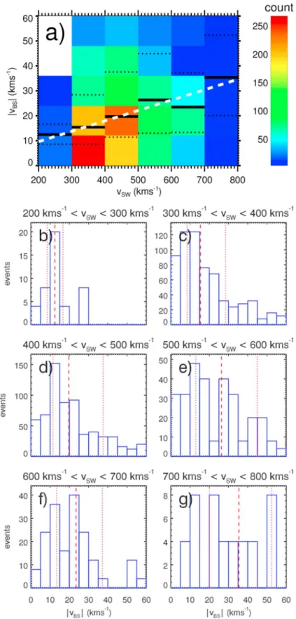
Figure 4. Statistical study of the bow shock speed. (a) 2-D histogram of the number of events as a function of bow
shock speed and the solar wind speed. Solid and dotted lines denote median values and the 25th/75th percentiles, respectively. A white dashed line shows a linear fit. (b)–(g) Histograms of bow shock speeds for six ranges of the solar wind speed. Dashed and dotted red lines denote median values and the 25th/75th percentiles, respectively.
Journal of Geophysical Research: Space Physics
10.1029/2018JA026272
of observations and over their spatial separation. For this reason, we have calculated also local𝜃mc
Bnand𝜃
mm
Bn
using Cluster measurements and compared their values with𝜃Bn. We have found that median values of
|𝜃mc
Bn−𝜃Bn| = 7.39◦and|𝜃Bnmm−𝜃Bn| = 6.07◦. Since all three methods of a𝜃Bndetermination provide similar
results, we can conclude that the investigated shocks do not exhibit significant local surface deformation. Our results suggest that the mixed method provides us with slightly more reliable results when compared to the magnetic coplanarity method which is consistent with previous studies (Echer, 2018; Tsurutani & Lin, 1985). We note that during large separation distances the effects of the bow shock curvature may affect the bow shock normal direction estimated from the timing analysis. However, we obtained similar values when we included only events with large spacecraft separation distances (>10,000 km, 75 events out of 529 or 14%):|𝜃mc
Bn −𝜃Bn| = 8.21◦and|𝜃mmBn −𝜃Bn| = 5.61◦. We thus conclude that the consistency between the
timing method and the magnetic coplanarity and mixed methods is maintained even at very large spacecraft separations.
In order to find how far is each particular bow shock crossing from the expected average position, we have analyzed observed bow shock locations using a three-dimensional bow shock model by Merka et al. (2005). This model is based on the set of approximately 550 bow shock crossings observed by 17 different spacecraft between 1963 and 1980. The bow shock model relies on average bow shock positions: Multiple nearby bow shock crossing positions were averaged into a single representative crossing. Therefore, its predictions tend to represent the (quasi-)stationary (steady and/or slowly changing upstream parameters) bow shock better than during rapid and significant changes in upstream conditions. It provides us a modeled radial distance
rmin a given direction defined by angles𝜃GPEand𝜙GPEparametrized by the upstream Alfvén Mach number
after normalizing for solar wind ram pressure. We have found that about a half of bow shock crossings are in agreement with this model within a 10% accuracy (i.e.,|r∕rm−1| ≤ 0.1). The accuracy of 20% and 50% are achieved in 78 % and 99% of cases, respectively. It indicates that the three-dimensional bow shock model by Merka et al. (2005) predicts well the bow shock locations over a wide range of angles and various upstream conditions.
We have compared the obtained bow shock speed with several solar wind parameters measured by Cluster-1. We did not find any significant correlation with the upstream pressure, density, Alfvén Mach number, nor with the magnetic field magnitude. The only parameter which seems to have a statistical influence on the bow shock speed is the solar wind speed. Figure 4a shows a 2-D histogram of the bow shock speed versus the solar wind speed. Our results suggest that the bow shock moves statistically faster during the periods of faster solar wind (the median and the 25th/75th percentile values follow the positive trend). We have also calculated a linear fit using obtained statistical parameters (a white dashed line in Figure 4a):|vBS| = (0.04 ±
0.01) × vSW+ (1.31 ± 3.86). The Spearman correlation coefficient is 0.73 for this data set (median values).
Figures 4b–4g display histograms of the bow shock speed for the six solar wind speed bins from Figure 4a. While we do not have many data points for the lowest and highest ranges (i.e., below 300 kms−1and above
700 kms−1), a reliable coverage is achieved for the four speed ranges in between. Figures 4b–4g confirm that
the bow shock speed variation with the solar wind speed is statistically significant. This can be explained by different properties of a fast solar wind originating in coronal holes, which has typically low plasma beta leading to higher magnetosonic speeds. When the bow shock is compressed by some disturbance in the upstream, the readjustment to equilibrium in a fast solar wind is more rapid due to the higher magnetosonic speed in the upstream, when compared to the slower one. El-Alaoui et al. (2004) discuss the possibility that the fast magnetosonic speed could be the upper limit of the bow shock speed during a magnetic cloud event. We have found that 99% of bow shock crossings are indeed below the upstream fast magnetosonic speed. However, we do not observe any significant correlation between the bow shock speed and the upstream fast magnetosonic speed (not shown).
Similar plots of the bow shock speed dependence on the𝜙GPEangle revealed a faster motion of the flank bow
shock (not shown). Additionally, we found that the increase of the bow shock speed toward flanks is about proportional to its mean standoff distance at a given local time. The differences between bow shock equilib-rium (model) positions and its recorded locations also increase toward flanks (see, e.g., Merka et al., 2005), suggesting that the bow shock speed could be correlated to the amplitude of its motion. The relative displace-ment of the crossing from its model position provides an estimate of the amplitude of the shock motion. For this reason, we have investigated a relation between the bow shock speed and a relative accuracy of the bow shock model predictions (Figure 5a). The positive sign of vBScorresponds to the bow shock motion toward
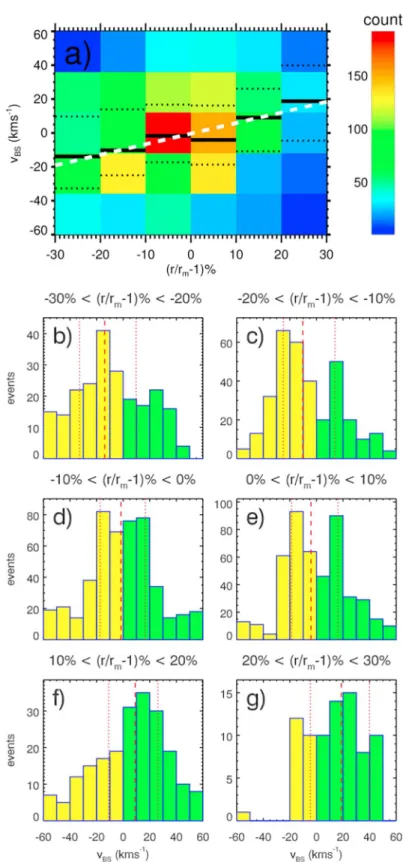
Figure 5. Statistical study of the bow shock speed and location. (a) 2-D histogram of the number of events as a function
of the bow shock speed and relative deviations between the observed bow shock radial distances and the modeled ones by Merka et al. (2005). Solid and dotted lines denote median values and the 25th/75th percentiles, respectively. A white dashed line shows a linear fit. (b)–(g) Histograms of bow shock speeds for six ranges of relative deviations between the observed bow shock radial distances and the modeled ones. Dashed and dotted red lines denote median values and the 25th/75th percentiles, respectively. Yellow/green bins represent sunward/earthward bow shock motion.
Journal of Geophysical Research: Space Physics
10.1029/2018JA026272
dashed line in Figure 5a): vBS = (0.62 ± 0.10) × (r∕rm−1)% − (0.36 ± 0.62). The Spearman correlation coef-ficient is 0.66 for this data set (median values). Figures 5b–5g show histograms of the bow shock speed for the six ranges of the relative bow shock accuracy from Figure 5a. We have a reliable coverage of data points in all bins suggesting that this variation is statistically significant. We have obtained a significant correlation between these two parameters. In other words, the bow shock observed closer to the Earth than predicted moves statistically faster toward the Sun and vice versa. We think that there can be two possible interpreta-tions of these observainterpreta-tions. The model predicts an equilibrium bow shock location. Large deviainterpreta-tions of the observed bow shock from predictions mean that the bow shock is far from the equilibrium due to an abrupt change of upstream parameters. Our results thus directly confirm a suggestion of Nemecek et al. (1988) that the bow shock speed is proportional to the magnitude of the jump in upstream conditions leading to the bow shock motion. On the other hand, broadness of the histograms in Figures 5b–5g do not depend on the separation between modeled and observed bow shock positions, whereas Nemecek et al. (1988) found a completely irregular bow shock motion for large jumps of upstream conditions. We believe that our result is more reliable because it is based on a precise determination of the bow shock speed and a direct mea-surement of upstream parameters. Our results indicate that the bow shock motion is mostly driven by the upstream conditions. We use the interplanetary magnetic field and solar wind parameters measured prior to outward (positive bow shock speeds) and after inbound (negative bow shock speeds) bow shock cross-ing. Providing that the bow shock motion is a consequence of an upstream pressure jump, we always use the post-jump pressure for the model position. Our analysis shows that the bow shock moves in the direc-tion toward the post-jump equilibrium locadirec-tion with the speed propordirec-tional to the relative deviadirec-tion from the model location (Figure 5). On the other hand, our results reveal that this model has a larger uncertainty for faster moving bow shocks. It can be related to larger fluctuations of upstream parameters which lead to bias in predicting the bow shock position. Obviously, such effect is proportionally smaller for slow to steady bow shocks. We suggest that the bow shock speed can be taken into account as a weighting factor for a new empirical bow shock location model.
4. Summary and Conclusion
We have performed the timing analysis of 529 terrestrial bow shock crossings observed by the four Cluster spacecraft between 2001 and 2013 in order to derive their normals and velocities along these normals. We demonstrate the data analysis using a bow shock detection from 19 March 2001 (Figure 1). Our measure-ments have a reliable coverage of the bow shock locations (Figure 2). Median value of the bow shock speed is 20 kms−1, but 10% of cases are found above 63 kms−1(Figure 3a). Analyzed bow shocks are
predomi-nantly quasiperpendicular due to the selection criteria employed in the study (Figure 3b). Deviations of the bow shock location from the Merka et al. (2005) three-dimensional bow shock model are about 10% in one half of the cases (Figure 3c). We have found a significant correlation between the bow shock and solar wind speeds (Figure 4). Relative deviations from the model bow shock location are correlated with the bow shock speed with possible implications for improving bow shock location models (Figure 5). Finally, we provide the bow shock list with retrieved speeds and normals as an Auxiliary material of this paper in JSON format, that can be used for further investigation by the community (supporting information Data Set S1).
References
Abraham-Shrauner, B. (1972). Determination of magnetohydrodynamic shock normals. Journal of Geophysical Research, 77, 736. https://doi.org/10.1029/JA077i004p00736
Balogh, A., Carr, C. M., Acuña, M. H., Dunlop, M. W., Beek, T. J., Brown, P., et al. (2001). The Cluster magnetic field investigation: Overview of in-flight performance and initial results. Annales Geophysicae, 19, 1207–1217. https://doi.org/10.5194/angeo-19-1207-2001 Colburn, D. S., & Sonett, C. P. (1966). Discontinuities in the solar wind. Space Science Reviews, 5, 439–506. https://doi.org/10.1007/
BF00240575
Eastwood, J. P., Hietala, H., Toth, G., Phan, T. D., & Fujimoto, M. (2015). What controls the structure and dynamics of Earth's magnetosphere? Space Science Reviews, 188, 251–286. https://doi.org/10.1007/s11214-014-0050-x
Echer, E. (2018). Solar wind and interplanetary shock parameters near Saturn's orbit (10 AU). Planetary and Space Science, 165, 210–220. El-Alaoui, M., Richard, R. L., Ashour-Abdalla, M., & Chen, M. W. (2004). Low Mach number bow shock locations during a magnetic cloud event: Observations and magnetohydrodynamic simulations. Geophysical Research Letters, 31, L03813. https://doi.org/10.1029/ 2003GL018788
Escoubet, C. P., Fehringer, M., & Goldstein, M. (2001). Introduction: The Cluster mission. Annales Geophysicae, 19, 1197–1200. https://doi.org/10.5194/angeo-19-1197-2001
Farris, M. H., & Russell, C. T. (1994). Determining the standoff distance of the bow shock: Mach number dependence and use of models.
Journal of Geophysical Research, 99(17), 681. https://doi.org/10.1029/94JA01020
Acknowledgments
The authors would like to thank the many individuals and institutions who contributed to making Cluster and CSA possible. O.K., J.Š., J.S., and F.N. acknowledge the support of the Czech Science Foundation grants 17-06065S, 16-04956S, 17-08772S, and 18-00844S, respectively. V.K. acknowledges support by an appointment to the NASA postdoctoral program at the NASA Goddard Space Flight Center administered by Universities Space Research Association under contract with NASA and the Czech Science Foundation grant 17-06818Y. O.S. acknowledges support from a grant LTAUSA17070. This work has been supported by the Praemium Academiae award. All the data used are listed in the references.
Formisano, V. (1979). Orientation and shape of the Earth's bow shock in three dimensions. Planetary and Space Science, 27, 1151–1161. https://doi.org/10.1016/0032-0633(79)90135-1
Horbury, T. S., Cargill, P. J., Lucek, E. A., Eastwood, J., Balogh, A., Dunlop, M. W., et al. (2002). Four spacecraft measurements of the quasiperpendicular terrestrial bow shock: Orientation and motion. Journal of Geophysical Research, 107(A8), 1208. https://doi.org/ 10.1029/2001JA000273
Jeˇráb, M., Nˇemeˇcek, Z., Šafránková, J., Jelínek, K., & Mˇerka, J. (2005). Improved bow shock model with dependence on the IMF strength.
Planetary and Space Science, 53, 85–93. https://doi.org/10.1016/j.pss.2004.09.032
Laakso, H., et al. (2010). Cluster Active Archive: Overview. Astrophysics and Space Science Proceedings, 11, 3–37. https://doi.org/10.1007/ 978-90-481-3499-1
Maksimovic, M., Bale, S. D., Horbury, T. S., & André, M. (2003). Bow shock motions observed with CLUSTER. Geophysical Research Letters,
30(7), 1393. https://doi.org/10.1029/2002GL016761
Mejnertsen, L., Eastwood, J. P., Hietala, H., Schwartz, S. J., & Chittenden, J. P. (2018). Global MHD simulations of the Earth's bow shock shape and motion under variable solar wind conditions. Journal of Geophysical Research: Space Physics, 123, 259–271. https://doi.org/ 10.1002/2017JA024690
Merka, J., & Szabo, A. (2004). Bow shock's geometry at the magnetospheric flanks. Journal of Geophysical Research, 109, A12224. https://doi.org/10.1029/2004JA010567
Merka, J., Szabo, A., Slavin, J. A., & Peredo, M. (2005). Three-dimensional position and shape of the bow shock and their variation with upstream Mach numbers and interplanetary magnetic field orientation. Journal of Geophysical Research, 110, A04202. https://doi.org/ 10.1029/2004JA010944
Meziane, K., Alrefay, T. Y., & Hamza, A. M. (2014). On the shape and motion of the Earth's bow shock. Planet and Space Science, 93, 1–9. https://doi.org/10.1016/j.pss.2014.01.006
Meziane, K., Hamza, A. M., Maksimovic, M., & Alrefay, T. Y. (2015). The Earth's bow shock velocity distribution function. Journal of
Geophysical Research: Space Physics, 120, 1229–1237. https://doi.org/10.1002/2014JA020772
Nemecek, Z., Safrankova, J., & Zastenker, G. (1988). Dynamics of the Earth's bow shock position. Advances in Space Research, 8, 167–170. https://doi.org/10.1016/0273-1177(88)90127-5
Parker, E. N. (1965). Dynamical theory of the solar wind. Space Science Review, 4, 666–708. https://doi.org/10.1007/BF00216273 Parks, G. K., Lee, E., Fu, S. Y., Lin, N., Liu, Y., & Yang, Z. W. (2017). Shocks in collisionless plasmas. Reviews of Modern Plasma Physics, 1,
1. https://doi.org/10.1007/s41614-017-0003-4
Peredo, M., Slavin, J. A., Mazur, E., & Curtis, S. A. (1995). Three-dimensional position and shape of the bow shock and their variation with Alfvenic, sonic and magnetosonic Mach numbers and interplanetary magnetic field orientation. Journal of Geophysical Research, 100, 7907–7916. https://doi.org/10.1029/94JA02545
Rème, H., et al. (2001). First multispacecraft ion measurements in and near the Earth's magnetosphere with the identical Cluster Ion Spectrometry (CIS) Experiment. Annales Geophysicae, 19, 1303–1354. https://doi.org/10.5194/angeo-19-1303-2001
Richardson, I. G., & Cane, H. V. (2012). Near-Earth solar wind flows and related geomagnetic activity during more than four solar cycles (1963–2011). Journal of Space Weather and Space Climate, 2(27), A02. https://doi.org/10.1051/swsc/2012003
Šafránková, J., Jelínek, K., & Nˇemeˇcek, Z. (2003). The bow shock velocity from two-point measurements in frame of the interball project.
Advances in Space Research, 31, 1377–1382.
Schwartz, S. J. (1998). Shock and discontinuity normals, Mach numbers, and related parameters. ISSI Scientific Reports Series, 1, 249–270. Spreiter, J. R., Summers, A. L., & Alksne, A. Y. (1966). Hydromagnetic flow around the magnetosphere. Planetary and Space Science, 14,
223. https://doi.org/10.1016/0032-0633(66)90124-3
Tsurutani, B. T., Lakhina, G. S., Verkhoglyadova, O. P., Gonzalez, W. D., Echer, E., & Guarnieri, F. L. (2011). A review of interplanetary discontinuities and their geomagnetic effects. Journal of Atmospheric and Solar-Terrestrial Physics, 73, 5–19. https://doi.org/10.1016/ j.jastp.2010.04.001
Tsurutani, B. T., & Lin, R. P. (1985). Acceleration of greater than 47 keV ions and greater than 2 keV electrons by interplanetary shocks at 1 AU. Journal of Geophysical Research, 90, 1–11. https://doi.org/10.1029/JA090iA01p00001
Tsurutani, B. T., & Rodriguez, P. (1981). Upstream waves and particles—An overview of ISEE results. Journal of Geophysical Research, 86, 4317. https://doi.org/10.1029/JA086iA06p04317
Tsurutani, B. T., Smith, E. J., Ho, C. M., Neugebauer, M., Goldstein, B. E., Mok, J. S., et al. (1995). Interplanetary discontinuities and Alfvén waves. Space Science Reviews, 72, 205–210. https://doi.org/10.1007/BF00768781