HAL Id: hal-01228958
https://hal.archives-ouvertes.fr/hal-01228958
Submitted on 18 Nov 2015HAL is a multi-disciplinary open access archive for the deposit and dissemination of sci-entific research documents, whether they are pub-lished or not. The documents may come from teaching and research institutions in France or abroad, or from public or private research centers.
L’archive ouverte pluridisciplinaire HAL, est destinée au dépôt et à la diffusion de documents scientifiques de niveau recherche, publiés ou non, émanant des établissements d’enseignement et de recherche français ou étrangers, des laboratoires publics ou privés.
Distributed under a Creative Commons Attribution - NonCommercial - ShareAlike| 4.0 International License
CASSINI/UVIS
Fernando J. Capalbo, Yves Bénilan, Roger V. Yelle, Tommi T. Koskinen, Bill
R. Sandel, Gregory M. Holsclaw, William E. Mcclintock
To cite this version:
Fernando J. Capalbo, Yves Bénilan, Roger V. Yelle, Tommi T. Koskinen, Bill R. Sandel, et al.. SOLAR OCCULTATION BY TITAN MEASURED BY CASSINI/UVIS. The Astrophysical journal letters, Bristol : IOP Publishing, 2013, 766 (2), pp.L16. �10.1088/2041-8205/766/2/L16�. �hal-01228958�
Fernando J. Capalbo and Yves B´enilan
Laboratoire Interuniversitaire des Syst`emes Atmosph´eriques (LISA), UMR 7583 du CNRS, Universit´es Paris Est Cr´eteil (UPEC) and Paris Diderot (UPD), 61 avenue du G´en´eral de
Gaulle, 94010, Cr´eteil C´edex, France
Roger V. Yelle, Tommi T. Koskinen and Bill R. Sandel
Lunar and Planetary Laboratory, University of Arizona, 1629 E. University Blvd., Tucson, AZ, USA
and
Gregory M. Holsclaw and William E. McClintock
Laboratory for Atmospheric and Space Physics, University of Colorado, 3665 Discovery Drive, Boulder, CO 80303, USA
ABSTRACT
We present the first published analysis of a solar occultation by Titan’s at-mosphere measured by the Ultraviolet Imaging Spectrograph (UVIS) on board Cassini. The data were measured during flyby T53 in April 2009 and correspond to latitudes between 21◦ to 28◦ south. The analysis utilizes the absorption of two solar emission lines (584 ˚A and 630 ˚A) in the ionization continuum of the N2 absorption cross section and solar emission lines around 1085 ˚A where absorp-tion is due to CH4. The measured transmission at these wavelengths provides a direct estimate of the N2 and CH4 column densities along the line of sight from the spacecraft to the Sun, which we inverted to obtain the number densities. The high signal to noise ratio of the data allowed us to retrieve density profiles in the altitude range 1120 - 1400 km for nitrogen and 850 - 1300 km for methane. We find an N2 scale height of ∼76 km and a temperature of ∼153 K. Our results are in general agreement with those from previous work, although there are some differences. Particularly, our profiles agree, considering uncertainties, with the density profiles derived from the Voyager 1 Ultraviolet Spectrograph (UVS) data, and with in situ measurements by the Ion Neutral Mass Spectrometer (INMS) with revised calibration.
Subject headings: occultations — planets and satellites: atmospheres — planets
and satellites: individual: (Titan) — space vehicles: instruments — instrumen-tation: spectrographs — Sun: UV radiation
1. INTRODUCTION
Titan’s atmosphere is composed mainly of N2 with a few percent of CH4. Knowl-edge of the distribution of these constituents with altitude, latitude, and longitude is key to constraining the atmospheric structure and dynamics, and thereby investigating energy and momentum balance in the upper atmosphere. This knowledge is used to develop and constrain models investigating atmospheric chemistry, aerosol production, thermal balance, and escape processes. Measurements by instruments on the Cassini spacecraft provide data necessary to study these processes. At present there are uncertainties about the absolute magnitude of the N2 densities in the upper atmosphere, with large disagreements among values inferred from in situ measurements by the Cassini Ion Neutral Mass Spectrometer (INMS) (Cui et al. 2009), from accelerometer measurements by the Huygens Atmospheric Structure Instrument (HASI) (Fulchignoni et al. 2005), and from the Attitude and Articu-lation Control System (AACS) on the Cassini spacecraft (Sarani & Lee 2009). Therefore, accurate and precise determination of the profiles of the main constituents is of primary importance.
Observation of occultations in the UV spectral region is a powerful technique for the study of upper atmospheres. In an occultation, radiation from the star is measured before and during the occultation of the star by the atmosphere. Occultation measurements can extend the altitude, latitude, and longitude range covered by in situ measurements, that are limited to the spacecraft trajectory. This complementarity is fundamental to map the variability of Titan’s atmosphere. Stellar occultations by Titan’s upper atmosphere observed in the FUV by the Ultraviolet Imaging Spectrometer (UVIS) on the Cassini spacecraft can constrain the distribution of hydrocarbons and aerosols in this region (Koskinen et al. 2011), but not N2, which absorbs only at shorter wavelengths. Cassini/UVIS also observes stellar and solar occultations in the EUV, which do measure the N2 absorption of Titan’s atmo-sphere. But stellar occultations are limited by absorption in the interstellar medium (ISM) to wavelengths longward of 911 ˚A, where absorption is by highly complex N2 electronic band systems (Lewis et al. 2008). Solar occultations observed in the EUV, on the other hand, measure absorption in the ionization continuum of N2 and the dissociation region of CH4, where cross sections vary smoothly with wavelength and have been precisely measured in the laboratory. Moreover solar occultations benefit from a better signal-to-noise ratio (S/N)
than stellar occultations. These data therefore are relatively straightforward to analyze and should provide reliable results, largely free from systematic uncertainties.
The first solar occultation by Titan was measured by the UVS instrument (Broadfoot et al. 1977) onboard the Voyager 1 spacecraft. Smith et al. (1982) used the data to confirm that the atmosphere is composed mainly of N2 with a small abundance of CH4. Their results were used to constrain several subsequent models of the upper atmosphere (e.g., Yung et al. (1984); Yelle (1991); Lara et al. (1996); Yelle et al. (1997)). A reanalysis of the Voyager solar occultation utilizing a more sophisticated analysis technique and an improved model for the instrument (Vervack et al. 2004) solved some inconsistencies noted by Strobel et al. (1992) in the Smith et al. (1982) opacity profiles. From their N2 and CH4 profiles Vervack et al. (2004) determined a temperature of (153 ± 5) K for the thermosphere.
In this work we present the first number density profiles of N2and CH4and temperatures in the thermosphere of Titan retrieved from a solar occultation observed by UVIS. The occultation took place during the T53 flyby. This flyby benefits from particularly good pointing stability and small attitude drift. Additionally, UVIS observed a stellar occultation during T53 (Koskinen et al. 2011), providing the opportunity to compare the CH4 densities derived from each observation. The methodology developed in the present work can be applied to other UVIS solar occultations to complement the temporal and spatial coverage from previous work and other instruments.
2. UVIS DATA REDUCTION
The UVIS EUV channel covers the 560 - 1180 ˚A spectral region. We refer the reader to Esposito et al. (2004) and references therein for a detailed description of the instrument. The T53 data, obtained from the Planetary Data System (PDS) website, consists of 1480 samples, each being a 1024 × 64 (spectral × spatial) array acquired at a 1 Hz cadence. The image of the Sun was defocused over the spatial dimension and the spatial pixels from lines 4-30 and 31-57 were summed into two bins for transmission to ground. We added the counts in these two lines (after applying the corrections described below) to obtain a wavelength bands × samples (or equivalently altitudes) matrix. For a description of the UVIS data and its processing see Capalbo (2010) and the UVIS User’s Guide accessible from the PDS Planetary Rings Node web site.
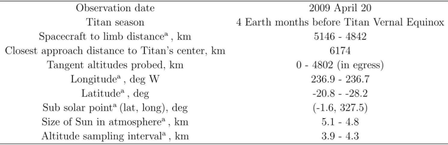
Flyby T53 took place on 20 April 2009. We retrieved reliable data for densities in the 849 - 1404 km region, near the evening terminator. The geometry of observation, including the tangent altitude or shortest distance between the UVIS line of sight and Titan’s surface,
Table 1: T53 observation characteristics.
Observation date 2009 April 20
Titan season 4 Earth months before Titan Vernal Equinox
Spacecraft to limb distancea, km 5146 - 4842
Closest approach distance to Titan’s center, km 6174
Tangent altitudes probed, km 0 - 4802 (in egress)
Longitudea, deg W 236.9 - 236.7
Latitudea, deg -20.8 - -28.2
Sub solar pointa(lat, long), deg (-1.6, 327.5)
Size of Sun in atmospherea, km 5.1 - 4.8
Altitude sampling intervala, km 3.9 - 4.3
aCorresponding to samples when the tangent altitude is between 849 - 1404 km.
was calculated by using the SPICE system developed by the Navigation and Ancillary In-formation Facility (NAIF) (Acton 1996). The Sun subtended an angle of 1 mrad in the field of view. Based on this and the imaging performance of the instrument (McClintock et al. 1993), the spectral resolution is estimated to be 3.6 ˚A. The size of the Sun projected onto the atmosphere is slightly larger than the altitude sampling interval (see Table 1). Therefore we choose to average every 2 samples to produce a net sampling distance of ∼8 km. This allows us to neglect the finite size of the Sun in subsequent analysis while increasing the SNR. The reduction of sampling rate has no significant effect on the final altitude resolution for derived local densities, as this resolution is dominated by the inversion of column densi-ties (Section 3). The parameters related to the observation geometry for T53 are given in Table 1.
Several steps are required to convert the raw data to useful physical measurements including wavelength calibration and registration and dark current and background subtrac-tion. Wavelength calibration is based on the position of well known solar emission lines (see Figure 1) and is performed individually on each spectrum because a pointing drift during the occultation caused a time and wavelength dependent shift of up to 1.3 ˚A in the recorded spectrum. We performed the wavelength correction separately for the two spatial lines in the binned data.
The unattenuated, raw solar spectrum contains instrumental background from several sources. The dark current and count values from the Cassini Radioisotope Thermoelectric
Generators (RTG) (Ajello et al. 2007) were negligible compared with other background counts. Contributions from other sources can be estimated from observations made when all solar light is completely extinguished by atmospheric absorption and is negligible at a rate 0.015 counts/sec/pixel. Furthermore, the spectral and temporal characteristics of the data reveal the presence of at least two types of scattered light. The first type varies with time in the same manner as the count rate at the long wavelength end of the spectrum. We therefore hypothesize that this background is due to light scattered by the instrument from longer wavelengths, probably including the intense solar Ly-α line. We subtract this background from the spectrum below 780 ˚A by assuming that it is proportional to the count rate in the 1100 - 1160 ˚A region, and requiring that the modified count rate in the 584 ˚A and 630 ˚A lines go to zero for altitudes where these lines have been extinguished by atmospheric absorption. Above 780 ˚A the average of the background in the 774 - 780 ˚A region was subtracted as a constant background. After these corrections a residual background remains, particularly next to the measured emission in 584 ˚A, 630 ˚A, and 1085 ˚A used in the analysis (see Figure 1). We interpret this background as extended wings of the instrument Point Spread Function (PSF). The temporal behavior of this second type of background is precisely the same as that of the spectral emissions features themselves; therefore, having no effect on the analysis, we do not correct for it.
The solar spectrum was measured by UVIS when the line of sight was outside the atmosphere. The spectrum shown in Figure 1 is an average of all the corrected samples corresponding to tangent altitudes from 2000 to 4800 km during T53. The spectrum consists mainly of intense solar lines, some continuum emission, and residual background. Figure 1 also shows the absorption cross sections of N2 (Gurtler et al. 1977) and CH4 (Kameta et al. 2002), the main EUV absorbers in Titan’s atmosphere. In this work we retrieve the density profiles of N2 and CH4 by using two bins centered on the solar lines at 584 ˚A (582.40 -586.63 ˚A) and 630 ˚A (627.79 - 631.43 ˚A) and a bin spanning solar lines around 1085 ˚A (1082.12 - 1088.19 ˚A), respectively. This retrieval procedure takes advantage of the facts that CH4 dominates absorption in the long wavelength bin, and that the cross sections do not change significantly in the wavelength bins used.
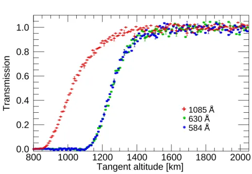
After the instrument corrections, the next step in the analysis is the calculation of the atmospheric transmission (Figure 2). Transmission is calculated by dividing the intensity measured at each tangent altitude by an unattenuated reference value; the latter being an average of the 290 values corresponding to tangent altitudes from 2000 km to 4800 km. These altitudes are safely beyond the region where absorption started to be evident at∼1500 km. The transmissions in the 584 and 630 ˚A bins are in excellent agreement, with half-light levels at 1256 km. The half-light level for the 1085 ˚A bin is at 1023 km. The 584 ˚A and 630 ˚A bins are absorbed much higher in the atmosphere than the 1085 ˚A bin because of the much
Counts 1000 100 10 10-16 10-17 10-18 Wavelength [A o] 1100 1000 900 800 700 600
Absorption Cross Section [cm
2 ]
CH4 Kameta et al. 2002 N2 Gurtler et al. 1977
Fig. 1.— Uncalibrated solar spectrum measured during the T53 flyby (top). N2 and CH4 absorption cross sections (bottom). The spectral bins used in the analysis are represented by the dashed vertical lines.
higher abundance of N2.
3. DATA ANALYSIS AND RESULTS
From the transmission in Figure 2 we derived column density profiles for N2 and CH4. As the 1085 ˚A bin is dominated by CH4 absorption, column densities along the line of sight,
N , are related to transmission through:
N =−ln(Tλ) σλ
= τλ
σλ
(1) where σλ is the absorption cross section and Tλ and τλ are the measured transmission and
optical depth of the atmosphere, respectively. The contribution of methane to the net optical depth is subtracted before the calculation of nitrogen column densities from the 584 ˚A and 630 ˚A bins. The ratio of the CH4 to N2 optical depths in these bins varies between 0.07 and 0.7 for altitudes between 1100 and 1400 km. The methane opacity was calculated using a linear fit to the natural logarithm of the derived column densities in the range 1100 -1300 km. The average values of the N2 absorption cross section in the short wavelength
Transmission
1.0
0.8
0.6
0.4
0.2
0.0
Tangent altitude [km]
2000
1800
1600
1400
1200
1000
800
+ 584 A o 630 A o 1085 A oFig. 2.— Transmission as a function of tangent altitude. The curves correspond to the wave-length bins used in the analysis, centered in the measured emission peaks whose wavewave-lengths are shown in the graph.
bins (see Figure 1) are (2.24±0.05)×10−17 and (2.34±0.07)×10−17 cm2 (from Samson et al. 1987). The average value of the CH4 absorption cross section in the long wavelength bin is (2.90±0.02)×10−17cm2. The column densities for N2 derived using the 584 ˚A and 630 ˚A bins and the CH4 column densities derived from the 1085 ˚A bin are shown in Figure 3. The upper boundary of the altitude range of the profiles is the lowest value with 100% uncertainty; the lower boundary corresponds to the lowest value in the transmission with S/N greater than 3. The N2 profiles derived from each bin agree within their uncertainties.
The problem of retrieving the number densities from the column densities is ill-posed and a direct inversion results in noise amplification. We solved this problem using a constrained linear inversion or Tikhonov regularization method (see for example Twomey 1977; Press et al. 1992), based on a second derivative operator to smooth the solution. Similar procedures have been used before (Vervack et al. 2004; Quemerais et al. 2006; Koskinen et al. 2011) and the technique presented here follows them closely. In the present work the column densities are first retrieved by direct inversion (no regularization). Then, the regularization matrix is set to an initial value based on the approach given in Press et al. (1992). The column densities are then recalculated iteratively multiplying the regularization matrix by 1.4 in every iteration until the norm of the difference between the column densities calculated from
Tangent altitude [km] 1400 1300 1200 1100 1000 900 Column densities [cm-2] 1017 1016 1015 1014 + 584 A o 630 A o 1085 A o
Fig. 3.— N2 and CH4 column density profiles derived from the transmission in Figure 2.
the retrieved number densities and the measured column densities is approximately equal to the norm of the uncertainties in the measured column densities. The consistency of the retrieval procedure was verified with simulated data. Results are shown in Figure 4. Nitrogen number densities in the boundaries of the altitude range have uncertainties bigger than 100% or altitude resolution several times bigger than the rest of the points, therefore they are not included in the results shown.
The regularization procedure reduces the altitude resolution of the result. This effect can be understood by examining the averaging kernel, the rows of which can be seen as smoothing functions (Rodgers 2000; Quemerais et al. 2006). Representative averaging kernels for the N2 and CH4 retrievals are shown in Figure 4 (averaging kernels for the two nitrogen bins are nearly identical). The full width at half maximum of the averaging kernels are approximately 25 km and 30 km for N2 and CH4 respectively.
The uncertainty of retrieved densities depends on the random noise in the spectrum, uncertainties introduced when inverting column densities into number densities, and the accuracy of the cross sections. Uncertainties in the column densities are calculated via error propagation, assuming a Poisson uncertainty for the raw data. The uncertainty in the number densities is derived from its covariance matrix, which is calculated as part of the inversion procedure. Uncertainty in the CH4 number densities varies from 11 to 5% in the
Tangent altitude [km]
1400
1300
1200
1100
1000
900
Number densities [cm
-3]
10
910
810
7 CH4 UVS solar occ. CH4 star occ. T53 CH4 INMS T55 CH4 INMS T51 CH4 solar occ. T53 N2 UVS solar occ. N2 INMS T55 N2 INMS T51 N2 HASI N2 solar occ. T53 N2 solar occ. T53 AVK 0.4 0.3 0.2 0.1Fig. 4.— N2 and CH4 number density profiles (filled circles). See text for references. Right plot: Averaging kernel (AVK) for a sample altitude, characterizing the altitude resolution of the nitrogen (blue) and methane (red) profiles.
range 850 - 1000 km region, increasing up to 50% near 1300 km. For N2, the uncertainty varies from 11 to 7% in the range 1120 - 1200 km region, and then increases up to 64 and 75% near 1400 km, for the densities derived from the 630 ˚A and 584 ˚A bins, respectively. The absorption cross sections contribute with a systematic uncertainty of 3% (Kameta et al. 2002; Samson et al. 1987) not included in the calculations described above. These N2 and CH4 cross sections are measured only at room temperature; therefore the variation of absorption coefficient with temperature is not accounted for in this study. This variation is expected to be small in the wavelength region used. For CH4 this argument is based on the behavior of the absorption cross section near 1200 ˚A (Chen & Wu 2004).
We used the number densities to derive the scale height and temperature. Fitting a straight line to the natural logarithm of our CH4 number densities between 920 and 1302 km we found a scale height of (100 ± 2) km. The scale height for the range 849 - 910 km
is (56 ± 3) km. The change in scale height is also evident in the stellar occultation data from Koskinen et al. (2011), also shown in Figure 4, but with a different slope below 920 km. Fitting straight lines to the natural logarithm of the N2densities in the range 1120 - 1404 km resulted in a scale height of (73± 2) and (76 ± 2) km using the 584 ˚A and 630 ˚A bin, respec-tively. If we assume an isothermal atmosphere these scale heights correspond to temperatures of (150± 4) K and (156 ± 4) K, in agreement with the 153 - 158 K found by Vervack et al. (2004) and 150 K found by Cui et al. (2009).
Comparison of our results with densities derived by other experiments is complicated by the possibility of temporal and geographic variations as well as differences in retrieval methods or uncertainties in instrument calibrations (see e.g. Cui et al. 2009). Nitrogen and methane densities measured at 1100 km by INMS can vary between Titan encounters by fac-tors of∼5.5 (Westlake et al. 2011) and ∼2.7 (Magee et al. 2009), respectively. Considerable variability in CH4 structure between flybys has also been observed from analysis of INMS data by Cui et al. (2012).
Our N2 densities are shown in Figure 4 together with values derived from measure-ments by different instrumeasure-ments, corresponding to different locations and times. The den-sity profile derived from the Huygens Atmospheric Structure Instrument (HASI) mass pro-file (Fulchignoni et al. 2005) assuming an atmosphere composed of nitrogen and 5% of methane, is a factor from 4.2 to 7.8 larger than our N2 profile. This discrepancy is larger than that expected based on the typical variability of the N2 density in the atmosphere, and remains to be explained. Although the N2 densities from Vervack et al. (2004), derived from UVS data, is a factor 1.6 to 2.8 larger than ours, our profile falls above their low un-certainty limit (not shown for clarity). These factors are similar to those associated with atmospheric variability as commented above. In fact, UVIS probed a different geographical location than UVS, 28 years later and under different solar activity conditions. The inbound and outbound INMS N2 number densities from flybys T51 and T55 (Cui et al. 2012), scaled from the original calibration by a factor of 2.9, are also shown in Figure 4. The T51 and T55 flybys took place about one month before and after T53, respectively. Although there are some discrepancies between our N2 profile and the INMS profiles, up to a factor of 1.7 in low altitudes, our results broadly agree with the INMS N2 densities measured during both flybys. The temporal and spatial variability of the N2 densities precludes us from providing strong constraints on the INMS calibration. Nevertheless, the agreement between our profiles and the INMS profiles shown suggests that the scaling factor of 2.9 is appropriate for N2.
Interestingly, our CH4 profile differs from the UVIS stellar occultation profile, measured for a different latitude of 39◦N on the dayside during T53 (Koskinen et al. 2011), by a factor of about 1.5 above 950 km. The profiles are closer at lower altitudes and coincide near
850 km. It is possible that the factor of 1.5 arises because the stellar and solar occultations probed different latitudes. Although the CH4 densities derived from UVS data differ from ours by a factor 0.8 to 2.5, our profile falls above their low uncertainty limit (not shown for clarity). Similar considerations to those for the discrepancies in N2 apply in this case. The inbound and outbound INMS CH4number densities from flybys T51 and T55 are also shown in Figure 4. These data have been scaled from the original calibration by a factor of 2.9. The difference between our values and the INMS profiles below 1140 km is a factor from 1.1 to 1.8. Above 1140 km our CH4 densities agree with those from INMS. The CH4 densities derived from the T53 stellar occultation differ from the T51 and T55 INMS density profiles by a factor of 2 - 3. This factor is in line with the variability discussed above.
4. SUMMARY
We present the first analysis of a solar occultation by Titan’s atmosphere observed with Cassini/UVIS. The densities shown are comparable to most of those presented in previous work, within factors 1 - 3. The derived temperature is comparable with that obtained from INMS and UVS measurements. The data presented here correspond to a location/period combination that was unexplored before, complementing the measurements of the upper at-mosphere made 28 years ago by Voyager 1/UVS and recently by Cassini/INMS and UVIS. Based on the dates and locations of the observations, the differences observed could be attributed to horizontal and temporal variations. However, the restricted sampling of the available data does not allow a firm conclusion on horizontal/seasonal variations. Future analysis of other solar and stellar occultations might fill in the spatial and temporal gaps among the data, and help to clarify if the differences observed are due to temporal or horizon-tal variations, or uncertainties in the measurements. In this context, the analysis could also benefit from future comparisons with densities derived from airglow measurements (Stevens et al. 2011).
RVY, TTK, and BRS acknowledge support from NASA grant NNX11AK64G. FJC acknowledges support from Universit´es Paris Est Cr´eteil through scholarship ‘Bourse de Mobilit´e’.
REFERENCES
Ajello, J. M., Stevens, M. H., Stewart, I., et al. 2007, Geophys. Res. Lett., 34, doi:10.1029/ 2007GL031555
Broadfoot, A. L., Sandel, B. R., Shemansky, D. E., et al. 1977, Space Sci. Rev., 21, 183 Capalbo, F. J. 2010, Master’s thesis, Lulea University of Technology/University Paul
Sabatier
Chen, F. Z., & Wu, C. Y. R. 2004, J. Quant. Spec. Radiat. Transf., 85, 195
Cui, J., Yelle, R. V., Strobel, D. F., et al. 2012, J. Geophys. Res., 117, doi:10.1029/2012JE004222
Cui, J., Yelle, R. V., Vuitton, V., et al. 2009, Icarus, 200, 581
Esposito, L. W., Barth, C. A., Colwell, J. E., et al. 2004, Space Sci. Rev., 115, 294 Fulchignoni, M., Ferri, F., Angrilli, F., et al. 2005, Nature, 438, doi:10.1038/nature04314 Gurtler, P., Saile, V., & Koch, E. 1977, Chem. Phys. Lett., 48
Kameta, K., Kouchi, N., Ukai, M., & Hatano, Y. 2002, J. Electron Spectrosc. Relat. Phenom., 123, 225
Koskinen, T., Yelle, R., Snowden, D., et al. 2011, Icarus, 216, 507, doi:10.1016/j.Icarus.2011.09.022
Lara, L. M., Lellouch, E., Moreno, J. J. L., & Rodrigo, R. 1996, J. Geophys. Res., 101, 23,261
Lewis, B. R., Heays, A. N., Gibson, S. T., Lefebvre-Brion, H., & Lefebvre, R. 2008, J. Chem. Phys., 129, 10.1063/1.2990656
Magee, B. A., Waite, J. H., Mandt, K. E., et al. 2009, Planet. Space Sci., 57, 1895
McClintock, W. E., Lawrence, G. M., Kohnert, R. A., & Esposito, L. W. 1993, Opt. Eng., 32
Press, W. H., Teukolsky, S. A., Vetterling, W. T., & Flannery, B. P. 1992, Fortran Numerical Recipes, Vol. 1, Numerical Recipes in Fortran 77, second edition edn. (Press Syndicate of the University of Cambridge)
Rodgers, C. D. 2000, Inverse methods for atmospheric sounding: theory and practice (World Scientific Publishing Co. Pte. Ltd)
Samson, J. A. R., Masuoka, T., Pareek, P. N., & Angel, G. C. 1987, J. Chem. Phys., 86, 6128
Sarani, S., & Lee, A. Y. 2009, in Proceedings of the AIAA Guidance, Navigation, and Control Conference (New York: Am. Inst. of Aeronaut. and Astronaut.), abstr. 5763
Smith, G. R., Strobel, D. F., Broadfoot, A. L., et al. 1982, J. Geophys. Res.
Stevens, M. H., Gustin, J., Ajello, J. M., et al. 2011, J. Geophys. Res., 116, doi:10.1029/2010JA016284
Strobel, D. F., Summers, M. E., & Zhu, X. 1992, Icarus
Twomey, S. 1977, Introduction to the Mathematics of Inversion in Remote Sensing and Indirect Measurements (DOVERM Publications), 0-486-69451-8
Vervack, J. R. J., Sandel, B. R., & Strobel, D. F. 2004, Icarus, 170, 91
Westlake, J. H., Bell, J. M., Jr., J. H. W., et al. 2011, J. Geophys. Res., 116, doi:10.1029/2010JA016251
Yelle, R. 1991, ApJ, 383, 380
Yelle, R. V., Strobell, D. F., Lellouch, E., & Gautier, D. 1997, in Huygens: Science, Payload and Mission, Proceedings of an ESA conference, ed. A. Wilson, 243 – 256, eSA SP-1177
Yung, Y. L., Allen, M., & Pinto, J. P. 1984, ApJS, 55, 465