Detection of Defects in FRP-Reinforced Concrete
with the Acoustic-Laser Vibrometry Method
by
Justin Gejune Chen
B.S. Physics
California Institute of Technology, 2009
Submitted to the Department of Civil and Environmental Engineering
in partial fulfillment of the requirements for the degree of
Master of Science in Civil and Environmental Engineering
at the
MASSACHUSETTS INSTITUTE OF TECHNOLOGY
February 2013
c
Massachusetts Institute of Technology 2013. All rights reserved.
Author . . . .
Department of Civil and Environmental Engineering
January 18, 2013
Certified by . . . .
Oral B¨
uy¨
uk¨
ozt¨
urk
Professor of Civil and Environmental Engineering
Thesis Supervisor
Certified by . . . .
Robert W. Haupt
Staff, MIT Lincoln Laboratory
Thesis Co-Supervisor
Accepted by . . . .
Heidi M. Nepf
Chair, Departmental Committee for Graduate Students
Detection of Defects in FRP-Reinforced Concrete with the
Acoustic-Laser Vibrometry Method
by
Justin Gejune Chen
Submitted to the Department of Civil and Environmental Engineering on January 18, 2013, in partial fulfillment of the
requirements for the degree of
Master of Science in Civil and Environmental Engineering
Abstract
Fiber-reinforced polymer (FRP) strengthening and retrofitting of concrete structural elements has become increasingly popular for civil infrastructure systems. When defects occur in FRP-reinforced concrete elements at the FRP-concrete interface, such as voids or delamination, FRP obscures the defect such that visual detection may not be possible. Most currently available non-destructive testing (NDT) methods rely on physical contact; an NDT method that is capable of remotely assessing damage would be greatly advantageous. A novel approach called the acoustic-laser vibrometry method which is capable of remote assessment of damage in FRP-reinforced concrete, is investigated in this thesis. It exploits the fact that areas where the FRP has debonded from concrete will vibrate excessively compared to intact material. In order to investigate this method, a laboratory system consisting of a commercial laser vibrometer system and conventional loudspeaker was used to perform tests with fabricated FRP-reinforced concrete specimens. The measurement results in the form of resonant frequencies were compared to those determined from theoretical and finite element defect models. With a series of measurements the vibrational mode shapes of defects and extent of the damage were imaged. The feasibility of the method was determined through a series of parametric studies, including sound pressure level (SPL), defect size, laser signal level, and angle of incidence. A preliminary Receiver Operating Characteristic (ROC) curve was determined for the method, and future work involving the acoustic-laser vibrometry method is proposed.
Thesis Supervisor: Oral B¨uy¨uk¨ozt¨urk
Title: Professor of Civil and Environmental Engineering Thesis Co-Supervisor: Robert W. Haupt
Acknowledgments
I would like to thank Rob Haupt and the rest of my old MIT Lincoln Laboratory team, Leaf, Marius, and Rich, for getting me started in working with laser vibrometry and its applications and really teaching me how to do this work. I’m thankful for my advisor, Professor Buyukozturk for introducing me to civil engineering and guiding me through my research.
Special thanks goes out to Tim Emge for helping me make measurements for supplying the FRP-steel specimen. John Doherty was also helpful in getting acquainted with the acoustic-laser vibrometry method. Also, I thank my previous group mates, Chakrapan and Denvid for their help and camaraderie.
This research was supported by the National Science Foundation (NSF), CMMI Grant No. 0926671, and I am grateful to the program managers, Dr. Mahendra Singh and Dr. Kishor Mehta for their interest in and support of this work. I also thank the American Society for Nondestructive Testing (ASNT) for their support through the 2011 Fellowship Award, and the opportunity to present this work at the 2012 Fall Conference.
Finally, I’m eternally grateful to my parents Yihwa and Minder for their encouragement and support in whatever endeavors I choose to pursue.
Contents
1 Introduction and Background 21
1.1 Infrastructure Assessment . . . 23
1.2 NDT of FRP-reinforced concrete . . . 24
2 Phenomenology and Theory 27 2.1 Concept . . . 27
2.2 Failure Modes of FRP-reinforced Concrete and Basic Phenomenology 28 2.3 Simplified Defect Model . . . 30
2.4 Rectangular Acoustic Cavity . . . 32
3 Finite Element Analysis 35 3.1 Sensitivity Analysis . . . 35
3.2 Plate Model Frequency Analysis . . . 40
3.3 Analysis With Air Void . . . 42
3.3.1 Air Void . . . 42
3.3.2 Concrete Void . . . 44
3.4 Analysis of Curved Plate . . . 46
3.5 Analysis of Curved Plate With Air Void . . . 49
3.6 Air Void Depth . . . 50
3.7 Summary: Finite Element Analysis . . . 52
4 Materials and Methodology 53 4.1 Fabrication of Concrete Test Specimens . . . 53
4.2 Summary of FRP-reinforced Concrete Specimens . . . 57
4.3 Experimental Setup . . . 63
4.4 Components of Laboratory Acoustic-Laser Vibrometry System and Key Specifications . . . 66
5 Defect Measurements 69 5.1 Preliminary Measurements . . . 69
5.2 Frequency Sweep Defect Measurements . . . 71
5.2.1 FRPP1 . . . 71 5.2.2 FRPP2 . . . 74 5.2.3 FRPC1 . . . 77 5.2.4 FRPC2 . . . 80 5.2.5 FRPCAD3 . . . 83 5.2.6 FRPC4 . . . 85 5.2.7 FRPP3 . . . 87 5.2.8 FRPP4 . . . 89 5.2.9 FRPP5 . . . 91
5.2.10 Summary: Frequency Sweep Defect Measurements . . . 97
5.3 Image Construction . . . 97 5.3.1 FRPP1 . . . 98 5.3.2 FRPP2 . . . 100 5.3.3 FRPC1 . . . 105 5.3.4 FRPC2 . . . 107 5.3.5 FRPC4 . . . 108 5.3.6 FRPP5 0.5” Defect . . . 113
5.3.7 Summary: Image Construction . . . 116
6 Parametric Studies 119 6.1 Sound Pressure Level . . . 119
6.2 Angle of Incidence . . . 121
6.4 Dwell Time . . . 124
6.5 Frequency Sweep Duration Study . . . 127
6.6 Summary: Parametric Studies . . . 128
7 Receiver Operating Characteristic Curve Analysis 129 7.1 ROC Curves . . . 129
7.2 Scaling of ROC Curve with Parametric Study Results . . . 134
7.3 Summary: ROC Curve Analysis . . . 137
8 Summary, Conclusions, and Future Work 139 8.1 Summary . . . 139
8.2 Conclusions . . . 140
8.2.1 Measurement Methodology . . . 140
8.2.2 Area Rate of Coverage . . . 141
8.2.3 Distance Limitations . . . 145
8.2.4 Defect Discrimination . . . 146
8.3 Future Work . . . 147
A Appendix 151 A.1 Chapter 5: Defect Measurements . . . 151
A.1.1 Frequency Sweep Defect Measurements . . . 151
A.2 Chapter 6: Parametric Studies . . . 155
A.2.1 Sound Pressure Level . . . 155
A.2.2 Dwell Time . . . 156
A.2.3 Frequency Sweep Duration Study . . . 160
A.3 Chapter 7: Receiver Operating Characteristic Curve Analysis . . . 162
List of Figures
1-1 I-35W Bridge After Collapse . . . 22
1-2 Corroded rebar and concrete spall, MIT Campus, West Garage . . . . 23
1-3 Damage in FRP reinforced bridge box-girder wall, Jamestown Bridge, RI . . . 25
2-1 Notional acoustic-laser vibrometry system for NDT . . . 28
2-2 Failure Modes of an FRP Strengthened RC beam . . . 29
2-3 Acoustic-Laser Vibrometry . . . 29
2-4 Mathematical Model of FRP Plate . . . 30
3-1 X-Eigenvector of mode 1,1 of a simply supported plate, f = 49.0608 Hz 36 3-2 X-Eigenvector of mode 2,2 of a simply supported plate, f = 196.2432 Hz 37 3-3 X-Eigenvector of mode 3,3 of a simply supported plate, f = 441.5471 Hz 37 3-4 Percent error vs. number of elements for mode 1,1 . . . 38
3-5 Percent error vs. number of elements for mode 2,2 . . . 38
3-6 Percent error vs. number of elements for mode 3,3 . . . 39
3-7 The plate finite element model, showing the eigenvector values for the first resonant mode . . . 41
3-8 Fourier analysis plot of the plate for out of plane vibration velocity at the center of the plate . . . 42
3-9 Diagram of the full defect as modeled . . . 43
3-10 Fourier analysis plot of the plate and air void for out of plane vibration velocity at the center of the defect . . . 44
3-11 Fourier analysis plot of the plate and concrete model for out of plane
vibration velocity at the center of the defect . . . 46
3-12 The curved plate finite element model, showing the eigenvector values for the first resonant mode . . . 47
3-13 Fourier analysis plot of the curved plate model for out of plane vibration velocity at the center of the defect . . . 48
3-14 The full curved defect as modeled . . . 49
3-15 Fourier analysis plot of the curved 1.5” × 1.5” plate and 1” air void for out of plane vibration velocity at the center of the plate . . . 50
3-16 The full defect as modeled for the air void thickness analysis . . . 51
4-1 Specimen mold and foam inserts . . . 54
4-2 Cast concrete specimen with foam inserts . . . 54
4-3 Cast concrete specimen with foam inserts removed . . . 55
4-4 Specimen after wet FRP-epoxy layup . . . 55
4-5 Completed FRP-reinforced concrete specimen . . . 56
4-6 FRPP0, FRP-bonded reinforced concrete panel . . . 58
4-7 FRPP1, FRP-bonded reinforced concrete panel . . . 58
4-8 FRPP2, FRP-bonded reinforced concrete panel . . . 59
4-9 FRPP3, FRP-bonded concrete panel . . . 59
4-10 FRPP4, FRP-bonded concrete panel . . . 60
4-11 FRPP5, FRP-bonded concrete panel . . . 60
4-12 FRPC1, FRP-confined concrete cylinder . . . 61
4-13 FRPC2, FRP-confined concrete cylinder . . . 61
4-14 FRPCAD3, FRP-confined concrete cylinder . . . 62
4-15 FRPC4, FRP-confined concrete cylinder . . . 62
4-16 Diagram of experimental setup . . . 63
4-17 Retroreflective tape adhered to specimen . . . 64
4-18 Light reflected from retroreflective tape on specimen, imaged onto paper surrounding the laser vibrometer lens . . . 64
4-19 Examples of measurement locations on specimen FRPP2 . . . 65
4-20 Sample measurement of sound pressure level of frequency sweep . . . 65
4-21 Polytec Laser Vibrometer OFV-505 and Controller OFV-5000 . . . . 66
4-22 M-Audio DSM1 Studio Monitor . . . 67
4-23 WaveBook/516E Data Acquisition System . . . 67
4-24 Earthworks M30 Microphone . . . 68
4-25 Earthworks 1021 Microphone Pre-amp . . . 68
5-1 Background measurement of FRPP0 . . . 70
5-2 Frequency sweep measurement of FRPP0 . . . 70
5-3 Frequency response of FRPP1 at center of defect . . . 72
5-4 Frequency response of FRPP1 at center side of defect . . . 72
5-5 Frequency response of FRPP1 at corner of defect . . . 73
5-6 Frequency response of FRPP1 over intact FRP-concrete system . . . 73
5-7 Frequency response of FRPP2 at center of defect . . . 75
5-8 Frequency response of FRPP2 at center side of defect . . . 75
5-9 Frequency response of FRPP2 at corner of defect . . . 76
5-10 Frequency response of FRPP2 over intact FRP-concrete system . . . 76
5-11 Frequency response of FRPC1 at center of defect . . . 78
5-12 Frequency response of FRPC1 at center side of defect . . . 78
5-13 Frequency response of FRPC1 at corner of defect . . . 79
5-14 Frequency response of FRPC1 over intact FRP-concrete system . . . 79
5-15 Frequency response of FRPC2 at center of defect . . . 81
5-16 Frequency response of FRPC2 at center side of defect . . . 81
5-17 Frequency response of FRPC2 at corner of defect . . . 82
5-18 Frequency response of FRPC2 over intact FRP-concrete system . . . 82
5-19 Frequency response of FRPCAD3 at center top of defect . . . 84
5-20 Frequency response of FRPCAD3 at center of defect . . . 84
5-21 Frequency response of FRPC4 at top of defect . . . 85
5-23 Frequency response of FRPC4 at bottom of defect . . . 86 5-24 Frequency response of FRPC4 over intact FRP-concrete system . . . 87 5-25 Frequency response of FRPP3 over defect . . . 88 5-26 Frequency response of FRPP3 over intact FRP-concrete system . . . 88 5-27 Frequency response of FRPP4 at center of defect . . . 89 5-28 Frequency response of FRPP4 over internally cracked region . . . 90 5-29 Frequency response of FRPP4 over intact FRP-concrete system . . . 90 5-30 Frequency response of FRPP5 over intact FRP-concrete system . . . 92 5-31 Frequency response of FRPP5 at center of 1” wide crack defect . . . 93 5-32 Frequency response of FRPP5 at center of 0.75” wide crack defect . . 94 5-33 Frequency response of FRPP5 at center of 0.5” wide crack defect . . . 95 5-34 Frequency response of FRPP5 at center of 0.25” wide crack defect . . 96 5-35 Frequency response of FRPP5 at center of 0.125” wide crack defect . 96 5-36 Surface plot of vibration amplitude for specimen FRPP1 at 3200 Hz,
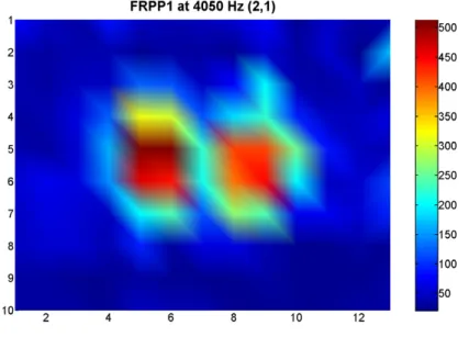
1,1 mode . . . 98 5-37 Surface plot of vibration amplitude for specimen FRPP1 at 4050 Hz,
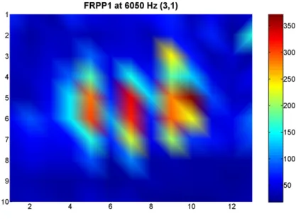
2,1 mode . . . 99 5-38 Surface plot of vibration amplitude for specimen FRPP1 at 6050 Hz,
3,1 mode . . . 100 5-39 Surface plot of vibration amplitude for specimen FRPP2 at 1380 Hz,
1,1 mode . . . 101 5-40 Surface plot of vibration amplitude for specimen FRPP2 at 1490 Hz,
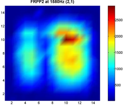
2,1 mode . . . 101 5-41 Surface plot of vibration amplitude for specimen FRPP2 at 1580 Hz,
2,1 mode . . . 102 5-42 Surface plot of vibration amplitude for specimen FRPP2 at 2050 Hz,
3,1 mode . . . 102 5-43 Surface plot of vibration amplitude for specimen FRPP2 at 2750 Hz,
5-44 Surface plot of vibration amplitude for specimen FRPP2 at 3260 Hz, 1,3 mode . . . 103 5-45 Surface plot of vibration amplitude for specimen FRPP2 at 3580 Hz,
2,3 mode . . . 104 5-46 Surface plot of vibration amplitude for specimen FRPP2 at 3940 Hz,
3,3 mode . . . 104 5-47 Surface plot of vibration amplitude for specimen FRPC1 at 4400 Hz,
1,1 mode . . . 105 5-48 Surface plot of vibration amplitude for specimen FRPC1 at 6040 Hz,
1,2 mode . . . 106 5-49 Surface plot of vibration amplitude for specimen FRPC1 at 8860 Hz,
2,1 mode . . . 106 5-50 Surface plot of vibration amplitude for specimen FRPC2 at 2740 Hz,
2,1 mode . . . 107 5-51 Surface plot of vibration amplitude for specimen FRPC2 at 3150 Hz,
1,1 mode . . . 108 5-52 Surface plot of vibration amplitude for specimen FRPC4 at 6300 Hz . 109 5-53 Surface plot of vibration amplitude for specimen FRPC4 at 8100 Hz . 109 5-54 Surface plot of vibration amplitude for specimen FRPC4 at 9090 Hz . 110 5-55 Surface plot of vibration amplitude for specimen FRPC4 at 10000 Hz 110 5-56 Surface plot of vibration amplitude for specimen FRPC4 at 11000 Hz 111 5-57 Surface plot of vibration amplitude for specimen FRPC4 at 12000 Hz 111 5-58 Surface plot of vibration amplitude for specimen FRPC4 at 13000 Hz 112 5-59 Surface plot of vibration amplitude for specimen FRPC4 at 14700 Hz 112 5-60 Surface plot of vibration amplitude for specimen FRPC4 at 16700 Hz 113 5-61 Plot of vibration amplitude for specimen FRPP5, 0.5” width defect at
9390 Hz . . . 114 5-62 Plot of vibration amplitude for specimen FRPP5, 0.5” width defect at
5-63 Plot of vibration amplitude for specimen FRPP5, 0.5” width defect at
11340 Hz . . . 115
5-64 Plot of vibration amplitude for specimen FRPP5, 0.5” width defect at 16300 Hz . . . 115
5-65 Plot of vibration amplitude for specimen FRPP5, 0.5” width defect at 20000 Hz . . . 116
6-1 Vibration amplitude of specimen FRPP1 vs. sound pressure level and fitted curve . . . 120
6-2 Vibration amplitude vs. angle of incidence for FRPP1 specimen . . . 121
6-3 Diagram of rippled FRPP1 surface measurement . . . 122
6-4 Vibration amplitude vs. angle of incidence for FRPS3 specimen . . . 123
6-5 Noise floor vs. fraction of light allowed through back into the laser vibrometer . . . 124
6-6 SNR and vibration amplitude as a function of dwell time for a sine wave excitation for FRPP1 . . . 125
6-7 SNR and vibration amplitude as a function of dwell time for a white noise excitation for FRPP1 . . . 126
7-1 Scatter plot data from FRPP1 grid measurement at 3200 Hz . . . 130
7-2 ROC curve for FRPP1 at 3200 Hz . . . 131
7-3 Plot of true and false positive rate vs. detection velocity level for FRPP1 at 3200 Hz . . . 131
7-4 ROC curve for FRPP2 at 1380 Hz . . . 133
7-5 ROC curve for FRPC1 at 4400 Hz . . . 133
7-6 ROC curve for FRPC2 at 3150 Hz . . . 134
7-7 Estimated effect of sound pressure level on FRPP1 ROC curve . . . . 135
7-8 Estimated effect of laser power or distance on FRPP1 ROC curve . . 135
8-1 Time required to measure 1 square meter vs. measurement spacing, 0.2s measurement time . . . 143 8-2 Time required to measure 1 square meter vs. measurement spacing,
with false positive time penalty . . . 144 8-3 Sound pressure level vs. Distance for commercial loudpseaker . . . 146 A-1 Frequency response of FRPP5 at center side long of 1” wide crack defect151 A-2 Frequency response of FRPP5 at center side short of 1” wide crack defect152 A-3 Frequency response of FRPP5 at corner of 1” wide crack defect . . . 152 A-4 Frequency response of FRPP5 at center side long of 0.75” wide crack
defect . . . 153 A-5 Frequency response of FRPP5 at center side short of 0.75” wide crack
defect . . . 153 A-6 Frequency response of FRPP5 at corner of 0.75” wide crack defect . . 154 A-7 Vibration amplitude of specimen FRPP2 vs. sound pressure level and
fitted curve . . . 155 A-8 Vibration amplitude of specimen FRPC1 vs. sound pressure level and
fitted curve . . . 155 A-9 Vibration amplitude of specimen FRPC2 vs. sound pressure level and
fitted curve . . . 156 A-10 SNR and vibration amplitude as a function of dwell time for a sine
wave excitation for FRPP2 . . . 156 A-11 SNR and vibration amplitude as a function of dwell time for a white
noise excitation for FRPP2 . . . 157 A-12 SNR and vibration amplitude as a function of dwell time for a sine
wave excitation for FRPC1 . . . 157 A-13 SNR and vibration amplitude as a function of dwell time for a white
noise excitation for FRPC1 . . . 158 A-14 SNR and vibration amplitude as a function of dwell time for a sine
A-15 SNR and vibration amplitude as a function of dwell time for a white noise excitation for FRPC2 . . . 159 A-16 Frequency Responses from FRPP1, 0.1 second long 0-20 kHz frequency
sweep . . . 160 A-17 Frequency Responses from FRPP1, 1 second long 0-20 kHz frequency
sweep . . . 160 A-18 Frequency Responses from FRPP1, 10 second long 0-20 kHz frequency
sweep . . . 161 A-19 Frequency Responses from FRPP1, 60 second long 0-20 kHz frequency
sweep . . . 161 A-20 Scatter plot data from FRPP2 grid measurement at 1380 Hz . . . 162 A-21 Plot of true and false positive rate vs. detection velocity level for
FRPP2 at 1380 Hz . . . 162 A-22 Scatter plot data from FRPC1 grid measurement at 4400 Hz . . . 163 A-23 Plot of true and false positive rate vs. detection velocity level for
FRPC1 at 4400 Hz . . . 163 A-24 Scatter plot data from FRPC2 grid measurement at 3150 Hz . . . 164 A-25 Plot of true and false positive rate vs. detection velocity level for
List of Tables
2.1 Table of values of frequency parameter λ for a clamped square plate . 31 2.2 Material Properties and Estimated Resonant Frequencies for a 1.5” ×
1.5” defect . . . 32 2.3 Material Properties and Estimated Resonant Frequencies for a 3.0” ×
3.0” defect . . . 32 2.4 Resonant frequencies for a 0.0381m × 0.0381m × 0.0254m closed box 33 3.1 Material properties for sensitivity analysis . . . 36 3.2 Finite element analysis derived resonant frequencies for a 1.5” × 1.5”
plate . . . 41 3.3 Material properties for air . . . 42 3.4 Finite element analysis calculated resonant frequencies for a 1.5” ×
1.5” plate over a 1.5” × 1.5” × 1” air void . . . 43 3.5 Materials properties values for concrete . . . 45 3.6 Resonant frequencies for the 1.5” × 1.5” curved plate and the percent
difference from the flat plate . . . 47 3.7 Resonant frequencies for the 3” × 3” curved plate and the percent
difference from the flat plate . . . 48 3.8 Calculated resonant frequencies for the curved 1.5” × 1.5” plate and
1” air void model . . . 49 3.9 Resonant frequencies of plate and air void model of varying air void
depth . . . 51 4.1 FRP system material properties . . . 53
4.2 Summary of Test Specimens . . . 57
4.3 Polytec Laser Vibrometer system specifications . . . 66
4.4 M-Audio DSM1 Studio Monitor specifications . . . 67
4.5 WaveBook/516E Data Acquisition System specifications . . . 68
4.6 Earthworks M30 Microphone specifications . . . 68
4.7 Earthworks 1021 Microphone Pre-amp specifications . . . 68
5.1 Visually determined resonant frequencies for specimen FRPP1 . . . . 74
5.2 Visually determined resonant frequencies for specimen FRPP2 . . . . 77
5.3 Visually determined resonant frequencies for specimen FRPC1 . . . . 80
5.4 Visually determined resonant frequencies for specimen FRPC2 . . . . 83
5.5 Visually determined resonant frequencies for specimen FRPCAD3 . . 85
5.6 Visually determined resonant frequencies for specimen FRPC4 . . . . 87
5.7 Visually determined resonant frequencies for specimen FRPP4 . . . . 91
Chapter 1
Introduction and Background
A large part of the United States infrastructure consists of buildings, bridges, roadways, tunnels, dams, and pipelines among many other structures. These structures need to be inspected and maintained to ensure their optimal function and to prevent failures that would impair the operation of the US economy [1]. It is already the case that much of the nation’s infrastructure is in need of desperate repair. More than 26% of the nation’s bridges are either structurally deficient of functionally obsolete, the condition of many of the nation’s estimated 100,000 miles of levees is unknown, and poor roadway conditions cost motorists $67 billion a year in repairs and operating costs [2]. These deficiencies in either inspection or maintenance have resulted in several high profile failures of critical structures.
The most recent well known example of a massive structural failure is the collapse of the I-35W highway bridge over the Mississippi River in Minneapolis, Minnesota as shown in Figure 1-1. Undersized gusset plates in the connections of the bridge from incorrect design, combined with a poor distribution of a much greater than average load led, to the sudden collapse [3, 4]. In addition to deficient design there is also the problem of damage which can only be detected through detailed inspection or may not be detectable.
Corrosion in reinforced-concrete structures is one such example. There have been documented cases of parking garages and bridges failing due to corrosion, causing significant property damage [5, 6]. Corrosion can also cause less
Figure 1-1: I-35W Bridge After Collapse [3]
catastrophic structural damage such as spall of the concrete cover, as seen in Figure 1-2, which also shortens the lifespan of the structure considerably, and in the case of structures such as overpasses and buildings which may have people and cars underneath, can be a dangerous failure mode. There are many documented cases of structural failures in the literature [7, 8, 9].
Figure 1-2: Corroded rebar and concrete spall, MIT Campus, West Garage
1.1
Infrastructure Assessment
There is a desperate need to detect damage in the structures that comprise the nation’s infrastructure to prevent costly failures from happening. Accurate detection of damage can determine whether or not a structure is in proper operational condition and locate defects to direct maintenance and rehabilitation efforts. There are two general categories of methods for assessing the condition of structures: structural health monitoring (SHM) and non-destructive testing (NDT). SHM is the detection of damage from observation of general characteristics, such as resonant frequencies, damping coefficients, and mode shapes, of the structure over time [10, 11]. By observing these general characteristics over time, the global health condition of the system, in theory, can be determined and continuously monitored. NDT, in general terms, is the examination of an ”object, material, or system without impairing its future usefulness” [12, 13]. The goal is to characterize an object in some way and detect damage or defects in an area local to the testing. A
rudimentary example of an NDT technique would be knocking on an object to see whether or not it is hollow [14]. They usually rely on fundamental physical characteristics of the object to detect damage. Technological innovations have expanded the scope of NDT and common techniques include acoustic, ultrasonic, magnetic, radiographic, thermographic, among others. Further technological development of NDT methods allows for better and faster detection of defects in materials and structures critical to the nation’s infrastructure.
1.2
NDT of FRP-reinforced concrete
The nondestructive evaluation of concrete is important to the maintenance and monitoring of highways, bridges, and many other civil infrastructure systems. However, it is difficult to evaluate certain types of concrete structures, in particular, fiber-reinforced polymer (FRP) reinforced or retrofitted concrete structures. FRP has been used since the 1990s to strengthen and retrofit concrete structures in civil infrastructure applications [15, 16, 17]. The issue with damage detection in an FRP-reinforced concrete system, is that the FRP cover conceals any voids, cracks, or delamination that may have formed in the concrete under the reinforcement. Examples of such damage are shown in Figure 1-3. Detection of defects is especially important in the case where FRP has been retrofitted to previously damaged structures and further damage is a distinct possibility.
There currently does not exist a robust standoff method for measuring such damage. Currently commercially available and recently researched NDT technologies for FRP-reinforced concrete include elastic wave, ultrasound, x-ray, and radar methods [19, 18, 20, 21]. These methods all share the disadvantage of requiring either contact or close proximity of equipment with the specimen under test.
Standoff methods of damage detection have numerous advantages over contact measurement methods since they allow for measurement of damage in locations that are physically difficult to access, such as high above the ground or over water. Also
Figure 1-3: Damage in FRP reinforced bridge box-girder wall, Jamestown Bridge, RI [18]
measurements covering a large area are simpler since the equipment can be swept along a surface or reaimed to measure a different location. Laser vibrometry is one method of standoff measurement that measures the velocity of a surface.
Laser vibrometry has the ability to measure the surface velocity of objects from relatively large distances. To first order, measurements of velocity are only limited by laser power and line of sight [22]. With the advent of commercial laser vibrometers, researchers without a background in optical systems have the opportunity to make use of them. Some applications of laser vibrometry in NDT include brake rotors and
engine manifolds among other things in the automotive industry [23], ripeness of fruit [24], land mine detection [25, 26, 27], bubbles in paint coatings [28], and damage in composite materials [29, 30].
There is a relevant body of previous work using the acoustic-laser vibrometry method that has been applied to the detection of landmines [25, 31], and the detection of damage in FRP-steel bonded systems [32, 33]. Immediately related work on the detection of damage in FRP-reinforced concrete with the method has been published by collaborators [34].
Chapter 2
Phenomenology and Theory
2.1
Concept
There is a general need for NDT methods that can be conducted from a distance because standoff capability confers numerous advantages as mentioned previously. At the most basic level, NDT uses some sort of excitation to elicit a response from the object being measured and uses differences in the response to discriminate between intact and damaged areas. Keeping this in mind, to form a standoff NDT technique methods for standoff excitation and measurement of the target are required. A laser vibrometer and an acoustic excitation can be combined to form a standoff system that is capable of locating and measuring defects in materials. When excited by the acoustic source, defective areas will vibrate with an amplitude greater than intact areas. The vibration amplitude of the surfance of the specimen is measured and depending on the response frequency and areas where the response is exaggerated, defects are located. It is a powerful technique that allows for non-contact measurement and can be made into a relatively compact and portable system. Conceptually, the system is meant to measure tall or difficult to reach structures such as bridge piers and highway overpass structures. Figure 2-1 is a conceptual diagram of how the system might work for measuring the condition of a bridge pier from shore. In this work the specific application of detecting defects in FRP-reinforced concrete is investigated.
Figure 2-1: Notional acoustic-laser vibrometry system for NDT
2.2
Failure Modes of FRP-reinforced Concrete
and Basic Phenomenology
In FRP-reinforced concrete there are a number of failure modes and defects that can occur as shown in Figure 2-2. The two types of damage the system is designed to detect are FRP debonding and void defects at the FRP-concrete interface. These are the two types of defects that result in the greatest difference in the surface vibration amplitude when the specimen is excited by an airborne acoustic wave at the surface. The measurement methodology exploits a variation in surface compliance due to these anomalies.
The debonding or delamination of FRP allows it to freely vibrate on the surface while in the case of intact material, epoxy firmly bonds the FRP to the concrete. When an FRP-reinforced concrete structure is stimulated by acoustic pressure waves from a loudspeaker or similar source, the area over a defect, will vibrate like a drum
Figure 2-2: Failure Modes of an FRP Strengthened RC beam [35, 36]
head as shown in Figure 2-3. Since the FRP is much thinner than the underlying concrete, elastic waves induced in the structure by the acoustic excitation will have a much greater vibration amplitude in the areas where the FRP is detached due to a defect, when compared to areas where the FRP-concrete system is intact. By using frequency sweeps for the acoustic excitation the specimen is excited over a wide band of frequencies. The laser vibrometer measures the surface vibration of the target, obtaining the vibration frequency response to locate and characterize any anomalies. Different defects will have different frequency responses and we can use this to approximately determine the size and shape of a detected defect.
2.3
Simplified Defect Model
To model a defect where the FRP has delaminated from the concrete in a certain area, a simplified mathematical model is considered: a square clamped plate, shown in Figure 2-4. Even though FRP is a directional material, for simplicity it is assumed to be isotropic. The air beneath the plate, which is much less dense and less ”stiff” than the FRP is also assumed to have a negligible effect on the resonant frequencies of the plate. The boundary where the FRP is bonded to the concrete is assumed to be a clamped boundary condition. The classical plate equation that describes this defect is in Equation 2.1 [37].
Figure 2-4: Mathematical Model of FRP Plate
D∇4w + ρh∂
2w
∂t2 = 0 (2.1)
D = 12(1−νEh32) = flexural rigidity of the plate
E = Young’s modulus h = thickness of the plate ν = Poisson’s ratio
ρ = density of the material
x,y, and time t
The resonant frequencies of the plate are determined by Equation 2.2.
f = λ 2πa2 s D ρh (2.2) λ = a frequency parameter
a = side length of the square plate f = resonant frequency
The value of frequency parameter λ is given in Table 2.1 for different vibrational modes, for the boundary condition and geometric shape, a square plate that is clamped on all sides [38].
Mode 1 2 3 4 5 6 1 35.999989 73.405 131.902 210.526 309.038 428 2 108.237 165.023 242.66 340.59 458.27 3 220.06 296.35 393.36 509.9 4 371.38 467.29 583.83 5 562.18 676 6 792.5
Table 2.1: Table of values of frequency parameter λ for a clamped square plate [38]
Using these equations, the expected resonant frequency of the different vibrational modes of the plate, assuming an isotropic material, can be calculated. Since fiberglass is not an isotropic material, so this method is only reasonable for giving an estimate of the fundamental resonant frequency. Using the following material property values, a table of resonant frequencies was calculated, shown in Tables 2.2 and 2.3. If the properties of the FRP being measured are known, from a measured resonant frequency, an estimation of the detect size can be back calculated.
Material Properties of FRP Calculated Resonant Frequencies Defect side length 0.0381 m Mode Frequency (Hz)
Young’s modulus 20.9 GPa 1,1 5151
Poisson’s ratio 0.2 2,1 10504
Density 1800 mkg3 2,2 15488
Thickness 1.3 mm 3,1 18875
Table 2.2: Material Properties and Estimated Resonant Frequencies for a 1.5” × 1.5” defect
Material Properties of FRP Calculated Resonant Frequencies Defect side length 0.0762 m Mode Frequency (Hz)
Young’s modulus 20.9 GPa 1,1 1288
Poisson’s ratio 0.2 2,1 2626
Density 1800 mkg3 2,2 3872
Thickness 1.3 mm 3,1 4719
Table 2.3: Material Properties and Estimated Resonant Frequencies for a 3.0” × 3.0” defect
2.4
Rectangular Acoustic Cavity
Now consider a cubic defect where there is a void in the concrete that is obscured by the FRP. The mathematical model for this defect is a rectangular box that is filled with air and this void will have specific resonant frequencies determined by the lengths of the sides of the box and the mode number, separate from those associated with the FRP plate covering the box. The resonance comes from the air vibrating inside the box. Resonant frequencies for the box are determined by Equation 2.3 [39]
f = ν 2 v u u t( l Lx )2 + (m Ly )2+ ( n Lz )2 (2.3)
ν = speed of sound in air
Lx, Ly, Lz = length, width, and depth of the box
l, m, and n = some non-negative integer corresponding to mode number
Assuming the speed of sound is 344.9392 m/s, the first couple of resonant frequencies for a box of size 0.0381m × 0.0381m × 0.0254m are calculated in Table 2.4.
l m n Frequency (Hz) 1 0 0 4526.76 1 1 0 6401.81 0 0 1 6790.14 1 0 1 8160.73 2 0 0 9053.52 1 1 1 9332.16
Table 2.4: Resonant frequencies for a 0.0381m × 0.0381m × 0.0254m closed box
Air is much less dense by approximately a factor of 103, and less stiff by a factor
of approximately 106 than FRP. Since the FRP plate is much more massive than the
volume of air in the void, the air is not able to ”move” the plate and so there should not be a large effect of the vibration of the air on the vibration of the plate. There may be some effect if the resonant frequencies of the plate and the void are very close, leading to some interaction between the two resonances, but in this example with these specific material and physical defect properties this is not the case.
In the case of more complex defects such as a model incorporating both the FRP plate, air void, and associated interaction, a curved plate, or any irregular defect shape, finite element analysis (FEA) is necessary to determine the resonant frequencies of the defect. These are examples of relevant situations in which simple closed form numerical or analytical solutions for the resonant frequencies are not possible or easily available.
Chapter 3
Finite Element Analysis
The best way to accurately obtain resonant frequencies for a given defect is to model the defect and loads in a finite element analysis (FEA) program. It is also the simplest way to calculate the resonant frequencies with many different defect configurations and loads because only the input geometry and settings need to be changed in the finite element analysis program. As long as an accurate mathematical model to approximate the real life defect is used in the finite element analysis, a reasonable estimation of the resonant frequencies can be obtained.
3.1
Sensitivity Analysis
Initially, a sensitivity analysis was performed to determine the effect of the mesh size on the resonant frequencies that result from the finite element analysis. The model used was a flat 3” × 3”, 1mm thick plate that is simply supported on all edges, which has an easily accessible closed form solution from classical plate theory. Three modes to compare the FEA generated results with the actual values were used. The material properties used here, given in Table 3.1 are different from the actual FRP properties used in the later FEA, however the sensitivity analysis still applies. Mode 1,1 has an analytically derived frequency of 49.0608 Hz, mode 2,2 with a frequency of 196.2432 Hz, and mode 3,3 a frequency of 441.5471 Hz. The three modes are shown in Figures 3-1, 3-2, and 3-3 respectively.
Side length 0.0762 m Young’s modulus 148 GPa Poisson’s ratio 0.0 Density of FRP 1.5e6 mkg3
Thickness of FRP plate 1mm
Table 3.1: Material properties for sensitivity analysis
In order to analyze the finite element method wed like to compare the number of elements used, and types of elements used. We will use shell elements for our finite element model since we already know that given this sort of thickness to length ratio of approximately 1/100, shell elements are far superior to 3D-solid elements [40]. Our finite element model is a square plate in the Y-Z plane. To have a simply supported boundary we have no translation but allow Y or Z rotation at the boundary. Since only the vibrational modes normal to the surface are relevant, degrees of freedom were restricted to X-translation, Y-rotation and Z-rotation.
Figure 3-1: X-Eigenvector of mode 1,1 of a simply supported plate, f = 49.0608 Hz
These modes were obtained from models with varying numbers of 4 and 9 node elements. Plots of the percent error vs. number of elements used for the model were obtained for the 1,1, 2,2, and 3,3, vibrational modes.
Figure 3-4 shows the error comparison for mode 1,1. 9 node elements allowed the value for f11 as calculated from the finite element model (FEM) to converge very
Figure 3-2: X-Eigenvector of mode 2,2 of a simply supported plate, f = 196.2432 Hz
Figure 3-3: X-Eigenvector of mode 3,3 of a simply supported plate, f = 441.5471 Hz
quickly. With only 2 elements across, or 4 elements total the first mode frequency was determined to within 1% of the actual value. With 4 elements across there was better than 0.1% error. When the error increases after the minimum at 5 elements it showed that the computation converged to some, slightly lower frequency than the analytical solution. Usage of 4 node elements allowed for a somewhat accurate solution with a relatively small number of elements, reaching 1% error with 10 elements on one side. Figure 3-5 shows the error comparison for mode 2,2. Again the use of 9 node
Figure 3-4: Percent error vs. number of elements for mode 1,1
Figure 3-5: Percent error vs. number of elements for mode 2,2
elements allowed for very quick convergence of the solution and a minimum error of 0.03% was obtained at 6 elements across one side. 1% error was obtained with 4 elements across and less than 0.1% error with 6 elements across. For 4 node elements the frequency reached 1% error at 20 elements. The solution did not converge nearly as quickly as when 9 node elements were used.
Figure 3-6: Percent error vs. number of elements for mode 3,3
Figure 3-6 shows the error comparison for mode 3,3. For 9 node elements, there was less than 1% error at 6 elements across one side and a minimum of 0.05% error at 8 elements across. Yet again, 9 node elements were very efficient at producing an accurate solution. For 4 node elements, 1% error was obtained at about 28 nodes. Again the convergence of the solution happened at about the same rate as previously and was outmatched by 9 node elements.
Summarizing the conclusions from the preceding plots, to obtain 1% error for the resonant modes of our simply supported plate, with 4 node elements the model needed about 20 elements in length per wavelength, while the 9 node elements only required about 4. This gives a rule of thumb to check if the mesh is fine enough for a certain vibrational mode. For 9 node elements a 0.1% error was obtained with about 6 elements across per wavelength. For a simulated analysis, as many 9 node elements as allowed by computational power will be used. These two guidelines determine an estimated maximum frequency that can be calculated accurately.
3.2
Plate Model Frequency Analysis
A finite element analysis on an FRP plate was conducted to confirm the model geometry and check agreement with plate theory. A commercial FEA software was used to conduct this analysis [40]. If there is good agreement, then it supports the argument that our method is reasonable. The model used for the FRP plate, was a square plate that is clamped on all sides. This approximated the delaminated FRP portion of the defect. The model consisted of a 7 × 7 grid of 9 node shell elements, which is a mesh size that is a compromise between computation speed and accuracy. Since the model has side length 0.0381 m, each shell element is 4.23 mm × 4.23 mm. For materials properties the values in Table 2.2 were used. The resulting frequencies of the plate from FEA were compared to those calculated in Chapter, also shown in Table 2.2.
To calculate the response, the model was run through 104 time steps of 10−5
seconds each, for a total time of 0.1 second. This resulted in a Nyquist frequency of 50 kHz. To approximate the frequency sweep, a pressure load of 0.2 Pa was applied on the surface of the plate model, with a frequency sweep from 0-20 kHz over the 0.1 second of the analysis. The 0.2 Pa of pressure corresponds to a sound pressure level (SPL) of 80 dB re 20 Pa which was a sound level that is close to that used in the experimental measurements. This excitation was used to determine the frequency response of the model under a uniform pressure load, similar to the specimen being excited by an acoustic wave with a frequency sweep waveform. Figure 3-7 shows a band plot of the displacement eigenvectors for the first resonant mode, which occurs at 5099 Hz.
The resonant frequencies as determined by finite element analysis and the difference from theory are shown in Table 3.2. The resonant frequencies from the plate model are in close agreement with theory. The model could be made more accurate at the expense of computational power, however it was already limited by the number of time steps necessary for the dynamically loaded analysis to approximate the experimental conditions.
Figure 3-7: The plate finite element model, showing the eigenvector values for the first resonant mode
Mode Frequency (Hz) Difference from theory
1 - 1,1 5098.71 -1.015% 2 - 2,1 10337.0 -1.59% 3 - 1,2 10337.0 -1.59% 4 - 2,2 15128.3 -2.322% 5 - 3,1 18461.9 -2.189% 6 - 1,3 18560.8 -1.665%
Table 3.2: Finite element analysis derived resonant frequencies for a 1.5” × 1.5” plate
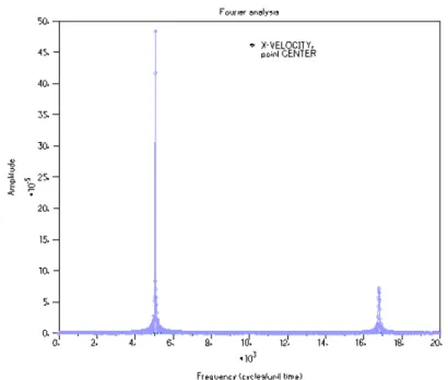
Figure 3-8 is a plot of the Fourier analysis of the response at the center of the plate model due to the frequency sweep loading. This shows the base resonant frequency at 5099 Hz of the plate. Note that the plate also responds at approximately 17 kHz which does not correspond to any of the resonant frequencies.
Figure 3-8: Fourier analysis plot of the plate for out of plane vibration velocity at the center of the plate
3.3
Analysis With Air Void
3.3.1
Air Void
Next, the defect was modeled as a system consisting of an air void and an FRP plate as shown in Figure 3-9. This more closely resembles the defect as it is in the experimantal FRP-reinforced concrete specimens. The basis for the model comes from an example problem presented previously in the literature [41]. The FRP plate is clamped on all sides, while the air void is clamped on 5 sides representing the boundaries of intact concrete, and on the remaining side it is constrained to move with the FRP plate. The same material properties as in the plate analysis for the FRP were used, and values used to define the properties of the air are given in Table 3.3.
Bulk modulus of air 1.404e5 Pa Density of air 1.18 mkg3
Air void dimensions 0.0381m × 0.0381m × 0.0254m Table 3.3: Material properties for air
Figure 3-9: Diagram of the full defect as modeled: FRP plate in red, air void in green
Mode Frequency (Hz) Vibrational mode
1 365.342 Free body motion of air
2 4520.31 1,0,0 mode of air void
3 4533.67 0,1,0 mode of air void
4 5024.34 1,1 mode of plate
5 6394.15 1,1,0 mode of air void
6 6885.26 0,0,1 mode of air void
7 8088.79 1,0,1 mode of air void
8 8115.71 0,1,1 mode of air void
9 9038.8 2,0,0 more of air void
10 9073.69 0,2,0 mode of air void
11 9303.84 1,1,1 mode of air void
Table 3.4: Finite element analysis calculated resonant frequencies for a 1.5” × 1.5” plate over a 1.5” × 1.5” × 1” air void
The plate part of the model consists of a 7 × 7 grid of 9 node shell elements as before. The air void part is a 7 × 7 × 2 grid of 27 node 3D solid elements. Again, they were constrained on one side to move together, to enforce the boundary condition at the FRP plate. The same loading on the model as the previous analysis to excite the model over a broad range of frequencies was used. Table 3.4 shows the resonant modes of the model and identifies them with respect to which part of the model they come from.
Figure 3-10 shows the response of the model at the center of the FRP plate to the frequency sweep. The air void resonances in the perpendicular directions did not
Figure 3-10: Fourier analysis plot of the plate and air void for out of plane vibration velocity at the center of the defect
contribute to the response of the model as measured on the surface of the FRP plate, however the 0,0,1 mode of the air void did contribute to the response in this model. This makes sense as that vibrational mode is in the direction of the measurement. In this case, the first resonant frequency of the plate that manifests itself in the response at 5024.32 Hz, was lower than that obtained from the model of only a plate at 5098.71 Hz. The air void effectively increased the mass of the plate, lowering the resonant frequency.
3.3.2
Concrete Void
To confirm the expected result when the FRP is properly bonded to the concrete, there is no response, concrete was substituted for the cavity of air. The material properties used for concrete are in Table 3.5 and the same material properties for the FRP were used.
The velocity response for the plate at the center over a similar ”void” composed of concrete is shown in Figure 3-11. The time step was reduced to 5×10⁻⁶seconds for
Young’s modulus of concrete 30 GPa Poisson’s ratio of concrete 0.2 Density of concrete 2400 mkg3
Table 3.5: Materials properties values for concrete
a Nyquist frequency of 100 kHz because the concrete is stiffer and therefore vibrates at a higher frequency. Note that the frequency axis now goes from 0 to 100 kHz.
The Fourier analysis plot in Figure 3-11 compared with Figure 3-10 for the plate over the air void, only above approximately 40 kHz was there a resonant frequency for the FRP plate over concrete. This resonant frequency was erroneous and was due to the mathematical model having a fixed boundary at the sides of the 1.5” × 1.5” × 1” box. The real world sample would not have that boundary because it would be a much larger concrete panel or cylinder and therefore would not resonate at that frequency. In this situation the plate vibration did not show up in the response because the concrete block is so much more massive than the FRP plate. This confirms the theory and measurements that a region of FRP-reinforced concrete without any defects will not exhibit any resonant frequencies and will look ”dead” to the laser vibrometer.
Figure 3-11: Fourier analysis plot of the plate and concrete model for out of plane vibration velocity at the center of the defect
3.4
Analysis of Curved Plate
The previous analysis covered defects on flat concrete panels, but a concrete column or cylinder provides a curved surface. The curved surface is expected to increase the stiffness of the FRP plate and therefore have a higher resonant frequency. Therefore, FEA was used to model a curved plate and a void covered by a curved plate to determine the effect on the frequency response.
The 1.5” × 1.5” FRP plate was modeled with a radius of curvature of 3” corresponding to the 6” diameter of our concrete samples. The plate is of the same size and has the same material properties as the flat plate modeled before. A band plot of the displacement eigenvectors for the first mode and picture of the model is shown in Figure 3-12.
The first resonant frequency was at 7940.6 Hz. This corresponded to a 56% increase in frequency over the flat plate caused by the increased stiffness of the curved plate. This was expected, because the curvature reduces the plate’s ability to deform, and effectively increases the stiffness. A list of the first couple of resonant modes and
Figure 3-12: The curved plate finite element model, showing the eigenvector values for the first resonant mode
frequencies of the plate is shown in Table 3.6.
Mode Frequency (Hz) Difference from flat plate
1 - 1,1 7940.6 56% 2 - 2,1 10690.6 3.4% 3 - 1,2 12139.8 17.5% 4 - 2,2 15775.7 4.3% 5 - 3,1 18695.0 1.3% 6 - 1,3 19652.8 5.9%
Table 3.6: Resonant frequencies for the 1.5” × 1.5” curved plate and the percent difference from the flat plate
Figure 3-13: Fourier analysis plot of the curved plate model for out of plane vibration velocity at the center of the defect
The same Fourier analysis was done on the plate loaded with a frequency sweep pressure load normal to the curved surface to determine the frequency response and the plot is shown in Figure 3-13. The 2,1; 1,2; and 2,2 modes did not contribute to the response since the center of the plate is on a nodal line for those vibrational modes.
Resonant modes for a 3” × 3” specimen were also determined are are shown in Table 3.7.
Mode Frequency (Hz) Difference from flat plate
1 - 1,1 3751.7 191.3% 2 - 2,1 4305.6 64.0% 3 - 1,2 5730.6 118.2% 4 - 2,2 5906.2 52.5% 5 - 3,1 6783.3 43.7% 6 - 1,3 7343.8 55.6%
Table 3.7: Resonant frequencies for the 3” × 3” curved plate and the percent difference from the flat plate
3.5
Analysis of Curved Plate With Air Void
A defect with a curved FRP plate covering the air void as shown in Figure 3-14 was also considered.
Figure 3-14: The full curved defect as modeled: FRP plate in red, air void in green
The model is the same as before with the 1.5” × 1.5” plate, except the top surface of the void is curved and the FRP is similarly curved. The resonant frequencies calculated by the finite element analysis program are given in Table 3.8. They were similar to that of the normal cubic defect, except for the increased frequency of the plate vibration.
Mode Frequency (Hz) Vibrational mode
1 533.9 Free body motion of air
2 4546.7 1,0,0 mode of air void
3 4674.9 0,1,0 mode of air void
4 6433.6 1,1,0 mode of air void
5 6509.6 0,0,1 mode of air void
6 7866.4 1,0,1 mode of air void
7 7936.8 1,1 mode of plate vibration
Table 3.8: Calculated resonant frequencies for the curved 1.5” × 1.5” plate and 1” air void model
To check that the first mode of plate vibration was indeed the main mode in the frequency response of the defect, a Fourier analysis of the response at the center of the plate was done as shown in Figure 3-15. The 7936.8 Hz first mode of plate vibration is the main response of the defect. This is only very slightly lower than in the case of the curved plate defect without the air void, showing that the air void has even less
effect on the vibration of the plate.
Figure 3-15: Fourier analysis plot of the curved 1.5” × 1.5” plate and 1” air void for out of plane vibration velocity at the center of the plate
3.6
Air Void Depth
An analysis of the void depth vs. resonant frequency was also conducted. As before, the defect was modeled as a system consisting of an air void and an FRP plate as shown in Figure 3-16. The FRP plate is clamped on all sides, while the air void is clamped on 5 sides representing the boundaries of intact concrete, and on the free side it is constrained to move with the FRP plate.
The plate part of the model consists of a 7 × 7 grid of 9 node shell elements as before. The air void part is a 7 × 7 × 3 grid of 27 node 3D fluid elements. They are tied together on one side to enforce the boundary condition at the FRP plate. For materials properties the same values as previously were used, as specified in Tables ?? and 3.3.
A simple frequency eigenvalue analysis was done for the models to obtain the resonant frequencies to be compared with that of just the clamped plate. The plate alone had a base resonant frequency of 5098.71 Hz. For the plate and air void model
Figure 3-16: The full defect as modeled for the air void thickness analysis: FRP plate in red, air void in green
Air void thickness (m) 4th Mode plate frequency (hz)
0.005 5183.56 0.01 5147.92 0.015 5101.89 0.02 5069.96 0.025 5033.05 0.03 4958.02
Table 3.9: Resonant frequencies of plate and air void model of varying air void depth
the fourth resonant mode corresponded to the same mode shape and vibrational mode as the base resonant mode of the clamped plate. Table 3.9 shows the resonant frequencies at the fourth mode for the finite element models with voids of varying depths.
When the air void was thin, the resonant frequency was actually higher than that of the clamped plate. With an air void depth of approximately half the side length, the frequency was close to that of the clamped plate, and when the air void was thicker, the resonant frequency was lower than that of the clamped plate. A possible explanation is that when the air void is thin, it acts as a spring increasing the effective stiffness of the plate, while when the air void is thick, the air adds mass to the plate, does not have much of a spring effect, and the resonant frequency is lowered. This means that once a defect is imaged, the measured resonant frequency
can be compared to the theoretical resonant frequency for a clamped plate of the same size and shape to possibly determine the approximate depth of the air void defect. The caveat is that diferences in frequency will most likely be differences in the defect geometry between the modeled and actual defect.
3.7
Summary: Finite Element Analysis
Finite element models were studied to see if they could be used to provide insight into the defect phenomenology. From the sensitivity study, for approximately 1% error in the resonant frequency when compared to analytical calculations, the finite element model needs to have a mesh density that provides 4 elements per wavelength with 9 node elements. Adding curvature to the plate increased the base resonant frequency because of a stiffening effect, and can be predicted by finite element analysis. The effect of an air void on the resonant frequency of the defect was quantified and studied. With a thinner air void the resonant frequencies are increased slightly, and with a thicker air void, the resonant frequencies are decreased slightly. With full knowledge and good modeling of the defect geometry, the thickness of the air void underneath the defect may be able to be quantified. In practice this will be difficult because of the lack of information about the true defect geometry necessary to determine if the frequency has shifted up or down from the plate only configuration.
Chapter 4
Materials and Methodology
4.1
Fabrication of Concrete Test Specimens
In order to test the system a series of FRP-reinforced concrete panels or cylinders with created defects were produced to simulate defects that might be measured in the real world. The FRP used was Tyfo SEH-51 composite, bonded to the concrete panel by wet lay-up with Tyfo S epoxy, from Fyfe co. Some specifications are given in Table 4.1. The following pictures illustrate the process of creating the specimens.
Material Properties Dry Fiber Epoxy Composite Laminate
Density (mkg3) 2550 1110
Tensile Modulus (GPa) 72.4 3.18 26.1 (test), 20.9 (design)
Laminate Thickness (mm) 1.3
Table 4.1: FRP system material properties [42]
Shown here was the process for the creating the FRPP5 specimen. First, foam was glued into a mold for casting the concrete specimen as in Figure 4-1. In this specific case, defects of multiple sizes are put into this mold, so that a study can be done to determine the minimum detectable crack size. Then, the concrete was cast in the mold and left to cure for at least one week, ideally a month, resulting in a concrete block with pieces of foam embedded in it as in Figure 4-2. Then, the pieces of foam were removed so that hollow voids were left in the concrete block as in Figure 4-3. Then the fiberglass was bonded to the concrete with epoxy using the wet
lay-up process as in Figure 4-4. The epoxy required a day to cure, and the resulting specimen is shown in Figure 4-5.
Figure 4-1: Specimen mold and foam inserts
Figure 4-3: Cast concrete specimen with foam inserts removed
4.2
Summary of FRP-reinforced Concrete
Specimens
There were two basic specimen types, either FRP-confined concrete cylinders, or FRP-bonded concrete panels. There were also two types of defects, a 1.5” × 1.5” × 1.0” cubic defect, and a 3” × 3” × 0.2” delamination-like defect, on both the cylinder and a panel specimen. This was used to study the effect of the curvature of the defect on the resonant frequencies observed by the system. Then, for the concrete cylinder specimens, there were specimens that have a 1” x 15” x 1” full length defect, and an irregular 1.5” × 5” delamination defect. For the concrete panels, there were specimens that have a 3” × 0.25” × 1.5” crack defect, a 3” × 0.25” × 1.5” 30◦ angled defect, and a panel that includes multiple sizes of crack defects, 3” × 0.125”, 0.25”, 0.5”, 0.75”, 1” × 1.5”. The specimens are summarized in Table 4.2, and described along with figures of the specimens below.
FRP-Confined FRP-Bonded Damage Type
Concrete Cylinder Concrete Panel
FRPP0 No damage
FRPC1 FRPP1 Cubic defect
FRPC2 FRPP2 Delamination-like defect
FRPCAD3 Full length defect
FRPC4 Irregular delamination defect
FRPP3 Crack defect
FRPP4 Angled crack defect
FRPP5 Multiple sizes of crack defects Table 4.2: Summary of Test Specimens
Figure 4-6: FRPP0, FRP-bonded reinforced concrete panel Size: Height 12” × Width 12” × Depth 4”
No defects
Figure 4-7: FRPP1, FRP-bonded reinforced concrete panel Size: Height 12” × Width 12” × Depth 4”
Figure 4-8: FRPP2, FRP-bonded reinforced concrete panel Size: Height 12” × Width 12” × Depth 4”
Delamination-like defect size: Height 3” × Width 3” × Depth 0.2”
Figure 4-9: FRPP3, FRP-bonded concrete panel Size: Height 7” × Width 13” × Depth 4”
Figure 4-10: FRPP3, FRP-bonded concrete panel Size: Height 7” × Width 13” × Depth 4”
Angled crack-like defect size: Height 0.25” × Width 3” × Depth 1.5”, approximately 30◦ angle
Figure 4-11: FRPP5, FRP-bonded concrete panel Size: Height 7” × Width 13” × Depth 4”
Multiple crack-like defect sizes: Height 3” × Widths 0.125”, 0.25”, 0.5”, 0.75”, 1” × Depth 1.5”
Figure 4-12: FRPC1, FRP-confined concrete cylinder Size: Height 12” × Diameter 6”
Cubic defect size: Height 1.5” × Width 1.5” × Depth 1.0”
Figure 4-13: FRPC2, FRP-confined concrete cylinder Size: Height 15” × Diameter 6”
Figure 4-14: FRPCAD3, FRP-confined concrete cylinder Size: Height 15” × Diameter 6”
Full length defect size: Height 15” × Width 1” × Depth 1”
Figure 4-15: FRPC4, FRP-confined concrete cylinder Size: Height 8” × Diameter 6”
4.3
Experimental Setup
Microphone Target
Specimen Laser Vibrometer
Acoustic Source Laser Vibrometer Controller Microphone Pre-amplifier Laptop Data Acquisition System
Figure 4-16: Diagram of experimental setup
The experimental setup involved a laser vibrometer, the loudspeaker, data collection equipment, and the sample under test. Figure 4-16 shows a diagram of the experimental setup. The laser vibrometer was a Polyec OFV-505 sensor head with an OFV-5000 controller, and the speaker was an M-Audio DSM1 with a ±3 dB frequency response of 49 Hz - 27 kHz. An Earthworks M30 omnidirectional microphone with 10 Hz - 30 kHz frequency response, was used to measure the sound pressure level at the target. The data acquisition system was an IOtech 516E WaveBook connected to a laptop, operating at a sampling frequency of 50 kHz for a Nyquist frequency of 25 kHz, more than sufficient for the maximum excitation frequency of 22 kHz. The arrangement of the equipment was such that the laser vibrometer measures the sample normal to its surface to avoid any errors in the vibration magnitude. The theory predicts a flexural vibration in the defect, so the maximum amplitude will be measured normal to the surface. The speaker was placed approximate one meter away from the sample and slightly off the line of sight of the laser vibrometer to avoid obstruction of the laser. The laser vibrometer was placed about three meters away from the sample, close enough to maintain good signal strength, while avoiding acoustic coupling from the speaker into the vibrometer. Retroreflective tape, as shown in Figure 4-17 was used on the specimens
to ensure a good return signal from the specimens for the laser vibrometer. It reflects incident light back in the direction of the laser vibrometer lens instead of scattering as it would off of a diffuse surface. A picture showing the reflected light is shown in Figure 4-18.
Figure 4-17: Retroreflective tape adhered to specimen
Figure 4-18: Light reflected from retroreflective tape on specimen, imaged onto paper surrounding the laser vibrometer lens
In order to determine the frequency response of the defect, measurements with the laser vibrometer were made in different locations, examples of which are shown
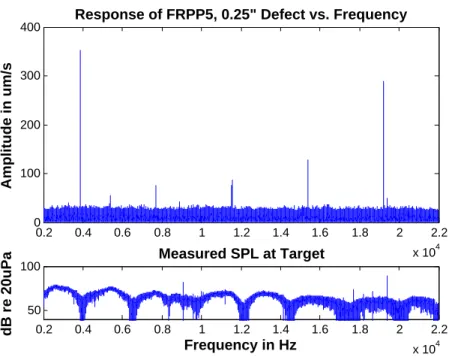
in Figure 4-19, while a frequency sweep was played on the loudspeaker. During the measurements the volume controls on the speaker were kept constant to maintain the same decibel level output. Amplitudes of the microphone and laser vibrometer measurement were scaled so that the resultant amplitude would be similar to that of a pure single frequency sine wave excitation. This amplitude scaling factor is the square root of the frequency sweep bandwidth times frequency sweep duration, which for a 20 kHz bandwidth and 60 second sweep duration, is 1095.445. A plot of the SPL measured at the sample as a function of frequency is shown in Figure 4-20.
Figure 4-19: Examples of measurement locations on specimen FRPP2
0.2 0.4 0.6 0.8 1 1.2 1.4 1.6 1.8 2 x 10⁴ 40 60 80 100 Measured SPL at Target dB re 20uPa Frequency in Hz
Figure 4-20: Sample measurement of sound pressure level of frequency sweep
From the calibration certificate, the M30 microphone is uniform to +1/-3 dB, and from the specifications the speaker is uniform to ±3 dB, which means that the ±10
dB uniformity of the sound power delivered to the target was likely a function of the acoustics of the room causing some frequencies to be louder than others. These variations in SPL were not great enough to cause the defect to respond with varying amplitudes that would look like a spurious resonant peak. The vibration velocity data was analyzed with a fast Fourier transform (FFT) to find resonance peaks that correspond to the resonant frequencies of the defect.
4.4
Components of Laboratory Acoustic-Laser
Vibrometry System and Key Specifications
The main components of the laboratory acoustic-laser vibrometry system and key specifications are given in the following figures and tables.
Figure 4-21: Polytec Laser Vibrometer OFV-505 and Controller OFV-5000 [43]
Maximum frequency 350 kHz (100 kHz used)
Measurement ranges 1 mm s V , 2 mm s V (used), 10 mm s V , 50 mm s V Laser wavelength 632.8 nm
Maximum stand-off distance 300m with OFV-SLR, surface dependent Typical spot size with OFV-LR lens 62 µm (1m), 135 µm (2m), 356 µm (3m) Resolution, Frequency dependent 0.01 - 0.04
µm s
√
Hz or 0.02 typical
Calibration error ±1%
Frequency dependent amplitude error ±0.05 dB
Figure 4-22: M-Audio DSM1 Studio Monitor [46] LF Driver 6.5-inch aluminum cone woofer HF Driver 1-inch soft teteron dome tweeter Frequency Response 49 Hz - 27 kHz ±3 dB
Max SPL @ 1 meter 110 dB maximum peak SPL @ 1m Dimensions H×W×D 12.8” × 9” × 10.3”
Table 4.4: M-Audio DSM1 Studio Monitor specifications [47]
Analog Inputs 8 differential
Resolution 16 bit
Maximum Frequency (per unit) 1 MHz
Ranges ±10V, ±5V, ±2V, ±1V
Accuracy ±5V: ±0.012% of reading; 0.006% of range
Total Harmonic Distortion -84 dB typ Signal to Noise and Distortion +74 dB typ
Dimensions W×D×H 11” × 8.5” × 2.7”
Table 4.5: WaveBook/516E Data Acquisition System specifications [48]
Figure 4-24: Earthworks M30 Microphone [49]
Frequency response 5Hz to 30kHz +1/-3dB Polar pattern Omnidirectional
Sensivitity 30mVP a (Typical), 34mVP a (Actual) Peak Acoustic Input 142dB SPL
Dimensions L×D 9” × 0.86”
Table 4.6: Earthworks M30 Microphone specifications [50]
Figure 4-25: Earthworks 1021 Microphone Pre-amp [49]
Frequency Response 2Hz to 100kHz ±0.1dB, 1Hz to 200kHz ±0.5dB Equivalent Input Noise -132dBV @ 20dB gain; -143dBV @ 60dB gain Max. Output Level +33dBu (37V peak-to-peak)
Dimensions H×W×D 1.75” × 9.5” × 10.3.75”
Chapter 5
Defect Measurements
5.1
Preliminary Measurements
Preliminary measurements were made on the specimen, FRPP0 that has no defects to confirm that there was no resonant frequency vibration response when the FRP-concrete system is intact. In these measurements no amplitude normalization constant was used so the amplitudes were the raw values from the laser vibrometer scaled by the 2000 micrometers per second, per Volt (
µm s
V ) scale factor. This scaling
factor was selected to ensure that the vibration would not clip during measurement. In the background measurement in Figure 5-1, the microphone records minimal background sound and the vibrometer has a flat noise floor except for three very narrow peaks. When a 60 second 0 - 20 kHz frequency sweep was used to excite the specimen as shown in Figure 5-2, the noise floor was actually lower, possibly due to a change in the laser signal received from the defect. Similarly three very narrow peaks were in the frequency response. Since they appear in both the passive background and active frequency sweep measurement, and they have very narrow widths, they must be due to some sort of noise in the system. If they are present in the passive background measurement where the specimen is not being acoustically excited, they are not due to a surface vibration of the specimen. Any resonance peak due to some physical measured feature, would have an associated damping, characterized in the frequency peak by the full width at half maximum (FWHM). Since the peaks were
0.2 0.4 0.6 0.8 1 1.2 1.4 1.6 1.8 2 x 10⁴ 0 20 40 Measured SPL at Target dB re 20uPa Frequency in Hz 0.2 0.4 0.6 0.8 1 1.2 1.4 1.6 1.8 2 x 10⁴ 0 0.1 0.2 0.3 0.4 0.5 0.6 0.7
Background Measurement of FRPP0 vs. Frequency
Amplitude in um/s
Figure 5-1: Background measurement of FRPP0
0.2 0.4 0.6 0.8 1 1.2 1.4 1.6 1.8 2 x 10⁴ 0 20 40 Measured SPL at Target dB re 20uPa Frequency in Hz 0.2 0.4 0.6 0.8 1 1.2 1.4 1.6 1.8 2 x 10⁴ 0 0.1 0.2 0.3 0.4 0.5 0.6 0.7 Response of FRPP0 vs. Frequency Amplitude in um/s